A log-periodic spiral antenna array for L-band radio interferometric imaging

Abstract

The perfect Y antenna array configuration is among the most prevalent antenna array arrangement used in radio interferometry for synthesis imaging. It is crucial to determine an antenna array configuration that could offer further higher quality radio-images. In this paper, a novel and an efficient L-band log-periodic spiral antenna array design is presented. The radio-imaging performance of the log-periodic spiral antenna array is compared and shown to outperform an equivalent perfect Y antenna array. Radio imaging performance is evaluated using the computational simulation for the proposed L-band log-periodic spiral antenna array and the equivalent perfect Y antenna array. The metric used for evaluation is the Structural Similarity Index (SSIM) and Surface Brightness Sensitivity (SBS). The L-band log-periodic spiral antenna array was observed to have about five times higher bandwidth, 2.24 times greater sensitivity, angular resolution better by a factor of five, and 10% wider field of view than the perfect Y configuration antenna array of comparable extent. It has been analytically demonstrated that the log-periodic spiral antenna array is an optimum configuration based on Chow’ s optimization technique. The L-band log-periodic spiral antenna array has outperformed the perfect Y configuration in many different imaging aspects.

Keywords

Radio telescope interferometry synthesis array log-periodic antenna array antenna array configuration

1 Introduction

Radio interferometric imaging is the primary technique used in space research to image astronomical bodies at radio wavelengths with high angular resolution. Radio interferometric imaging has been adopted for satellite earth observation. Example applications include soil moisture and ocean salinity measurements (and stand-off radio-frequency (RF) detection systems) [1 –4]. However, optical interferometry is extensively used in applications requiring shorter wavelengths than radio waves, such as biomedical imaging [5 –7]. A radio interferometer is made up of at least two antennas and in practice, consists of a few tens of antennas. These antennas are arranged in a specific geometrical fashion, and the arrangement is called an antenna array configuration [8].

The antenna array configuration significantly influences the quality of the radio image produced by the interferometer. Each of the antenna pairs in the configuration forms a baseline. The trajectory of baseline projection on the “spatial frequency plane” due to the earth rotation (or the relative motion of satellite for the earth in the scenario of earth imaging) creates baseline tracks [9, 10]. The baseline tracks should sample the maximum relevant number of points in the “spatial frequency plane” [9] for the best imaging performance. Thus it can be seen that the ensemble of baselines, which in turn is decided by the antenna array configuration, determines the image quality.

Though the subject of spiral antenna array design performance has been dealt upon by quite a few researchers [11 –13] they have restricted their performance evaluation using “anticipative assessment techniques” [14] in the uv-plane, such as determination of uv-coverage and sidelobe level. However, the final test of an antenna array design is its imaging performance achieved by assessment in the image-plane [14], which is a projected two-dimension distribution of the radio sky. Nonetheless, evaluation in the image-plane demands reliable image assessment metrics [15]. A conventional image assessment metric is Mean Squared Error (MSE) [16], although it does not equate with the human-perceived visual quality [16]. Hence, image plane assessment could be applied reliably only by employing human beings and is thus a subjective measure. Nevertheless, in the past two decades, tremendous progress in computer vision has been achieved and has primarily evolved based on the study of the operation of human visual systems (HVS) [17]. The structural similarity index (SSIM) is a widely adopted image quality evaluation metric by the image processing community [18]. It is developed along with the philosophy of differentiating images using the structural information present in them, just as the ways humans do [16] and hence is highly reliable. The spiral antenna array design that has been proposed makes use of SSIM in the radio imaging domain along with approaches such as Surface Brightness Sensitivity (SBS) [19].

An in-depth comparative analysis of a spiral antenna array design is being reported here, specifically in the image-plane and in the L-band. The L-band is suitable for earth radio interferometric imaging typically made at 1.4 GHz [20]. In Section 2, some of the related works are reviewed. Section 3 briefs on Chow’s solution for an optimum array configuration [9]. Further, in Section 4 and Section 5 observations, i.e., images generated by the two antenna arrays and the subsequent analysis of observed data, are described respectively. Results obtained have been discussed in Section 6. Finally, a summary of work and conclusions are provided in Section 7.

2 Related work

Numerous geometrical shapes have been used for antenna array design across the world. These include the T-array [21], the Y shaped array [21], randomly distributed antenna arrays [8], reuleaux triangle [22], spiral-shaped array, donut or double-ring arrays [23] and other “ringlike” arrays [24].

The Y shaped array, specifically the perfect Y configuration is a widely adopted antenna arrangement. Example configurations are The Very Large Array (VLA) (New Mexico, United States) and the Microwave Imaging Radiometer by Aperture Synthesis (MIRAS) [25] and Giant Metrewave Radio Telescope (GMRT). The MIRAS is an earth observation radio interferometric system. The GMRT uses a deformed Y configuration.

John Conway was among the first who made an in-depth investigation of a spiral antenna array design [11]. He discovered that it rendered strongly tapered uv-coverage and compared well with the antenna arrays existing then [11]. Subsequently, the spiral antenna array design was considered as a candidate for the Atacama Large Millimeter Array (ALMA) [12].

Despite wide adoption of Y configuration, simulation studies done as part of the square kilometer array (SKA), world’ s future largest radio telescope, reveal that uv-coverage metric δu/u provided by the spiral antenna array is 0.219, which is better than the perfect Y antenna array which has δu/u of 0.072 [13, 26]. However, such studies confine the analysis to the spatial domain and do not take advantage of analysis in the image-plane.

3 An optimum solution to the “configuration problem”

Array As mentioned previously, the antenna array configuration employed in a radio interferometer significantly influences the quality of the radio image generated by the interferometer. The notion of obtaining an optimum antenna array configuration is referred to as solving the “configuration problem” [8].

An optimum solution to the “configuration problem” has been given by Chow [9]. According to Chow, an optimum solution is achieved when the radial distance of the antenna elements, r in an antenna array configuration, is inversely proportional to 3D track density, which is in-turn inversely proportional to 2D baseline density (Eq. (1) [9], Equation (2) [9]). $r \propto \frac{1}{3 D track density}$ (1) $\Rightarrow r \propto \frac{1}{2 D baseline density}$ (2)

4 Observations

Observations were conducted by computational simulation. An example log-periodic spiral antenna array configuration with the dots representing the location of the antenna is shown in Fig. 1. In the example antenna array, the number of antenna elements, M is 27, the innermost radius, r_i is 0.1 units, the outer most radius, r_o is 0.5 units, and the angular spacing between adjacent elements, θ_s is 60°. The antenna location in polar co-ordinates for a log-periodic spiral antenna array is given by Equation (3)-Eq.(5) [27]. 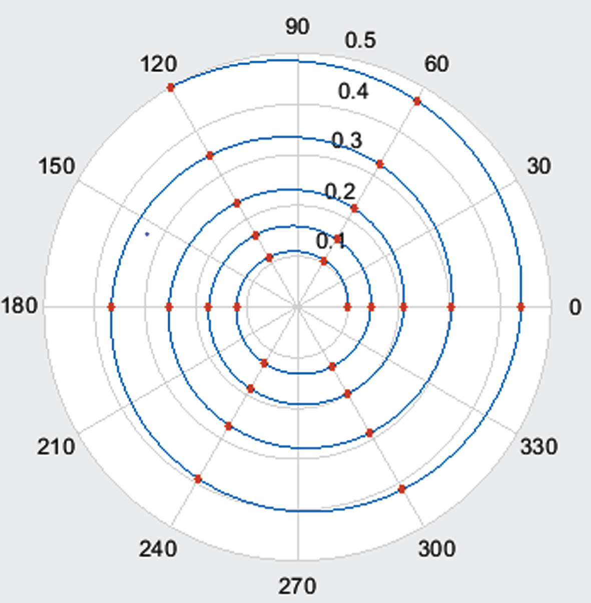$(r_{i} e^{bk θ_{s}}, k θ_{s})$ (3) $b = \frac{1}{M θ_{s}} \ln (\frac{r_{o}}{r_{i}})$ (4) $k = 0, 1, . . ., M .$ (5)

Fig. 1

A log periodic spiral antenna array. The dots represent the antenna location. Adjacent antennas along the spiral trajectory have equal angular spacing.

As per Equation (3), the inner spiral radius, r_i and the angular spacing between adjacent elements, θ_s are parameters that need to be resolved for further advancing the radio imaging performance of a log-periodic spiral antenna array. Hence, observation data requires to be generated for two objectives, namely (i) Maximizing radio imaging performance of a log-periodic spiral antenna array and (ii) Comparing the imaging performance of the optimized log-periodic spiral antenna array with the perfect Y antenna array. Observation data was generated using the image shown in Fig. 2 as the reference test radio source (the “actual image”). The pixel values of the “actual image” represent the surface brightness distribution of the test radio source.

Fig. 2

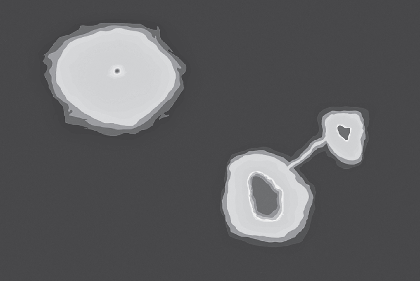
Reference image used for generating observations using radio interferometer simulator [28].

The test image was provided as an input to APSYNSIM (Aperture Synthesis Simulator) [28], a radio interferometer simulator. The radio interferometer simulator can be configured to simulate an appropriate antenna array, using an antenna-array configuration data-file. Antenna-array configuration data-file has provisions to define observing frequency, integration time, antenna diameter, and antenna positions. Further, the size of the test image can be specified using a source configuration data file. APSYNSIM, using an antenna-array configuration data-file, source configuration data file, and the “actual image” (test image), performs radio interferometric simulation to produce the corresponding observed image (“dirty image”).

Imaging configuration parameters defined by configuration data files is listed in Table 1. The configuration data is used by the simulator to produce observed images. The frequency response, integration time response, and angular resolution are the imaging performance parameters. For frequency response and integration time response, observation data was generated for both earth imaging from a space platform and space imaging from the earth. For space imaging, the antenna array radius and antenna diameter were assigned the values 20 km and 25 m, respectively, while for space imaging, these values were 20 m and 5 mm, respectively. Frequency response is obtained by varying the observing wavelength from 5 mm to 225 mm in steps of one mm with other parameters assigned values, as shown in Table 1. Four hundred forty-two observed images were generated for an antenna array to evaluate frequency response. Similarly, the integration time response was obtained by varying integration time from 0.2 to 9 hours in steps of 0.1 hours. A total of 178 observed images per antenna array was generated. The test image size was varied to evaluate angular resolution. A total of 1440 observations (720 per antenna array) were obtained for the evaluation of imaging performance. Besides, for optimization of the spiral antenna array, 300 observed images were generated with a cumulative sum of 1740 observations. Example observations are shown in Fig. 3(a)-(f).

Table 1

Imaging configuration parameters	Spiral antenna array optimization	Frequency response	Integration time response	Angular resolution
Number of antenna	27	27	27	27
Observing wavelength (mm)	211.26	5 - 225	211.26	211.26
	(1.42 GHz)	(in steps of 1 mm)	(1.42 GHz)	(1.42 GHz)
Integration Time (hour)	6	6	0.2 - 9 (in steps of 0.1 hour)	6
Test image size	120 arc sec^*	120 arc sec^*,	120 arc sec^*,	6 - 600 (in steps
		100000 arc sec†	100000 arc sec†	of 6 arc sec)
Antenna array radius	20km^*	20km^*,20m†	20km^*,20m†	20km^*
Antenna Diameter	25m^*	25m^*,5mm†	25m^*,5mm†	25m^*
Innermost spiral radius (km)	0.1,0.5,0.9,1.3,1.5	-	-	-
Angular spacing (degrees)	3-180	-	-	-
	(in steps of 3°)
Total number of observations	300	442	178	100

*Used for space imaging from earth.

† Used for earth imaging from space.

Fig. 3

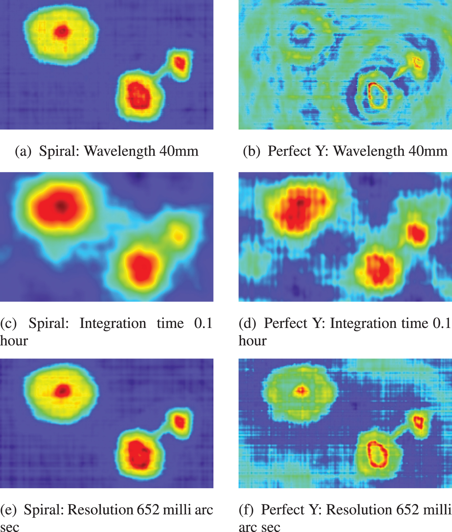
Observed example images. Top panel: Frequency response. Middle panel: integration time response. Bottom panel: Angular resolution [28].

5 Data analysis

As discussed beforehand, a total of 1740 observations were obtained for the evaluation of imaging performance, which required 1640 configuration data files and 1740 executions of APSYNSIM. To ease the task of obtaining the observation data and the subsequent data analysis, an automation framework, depicted in Fig. 4, was developed and employed by our team. As shown in Fig. 4, the Automated Execution Engine invokes the automatic execution of the radio interferometer simulator, APSYNSIM. The radio interferometer simulator can be configured to simulate different antenna array or source configuration. APSYNSIM, using the configuration files and the “actual image” performs radio interferometric simulation to produce “dirty image” and an SBS metric for the run. PYSSIM (Python module for SSIM) [29], the image comparator compares the “actual image” and “dirty image” to output an SSIM metric.

Fig. 4

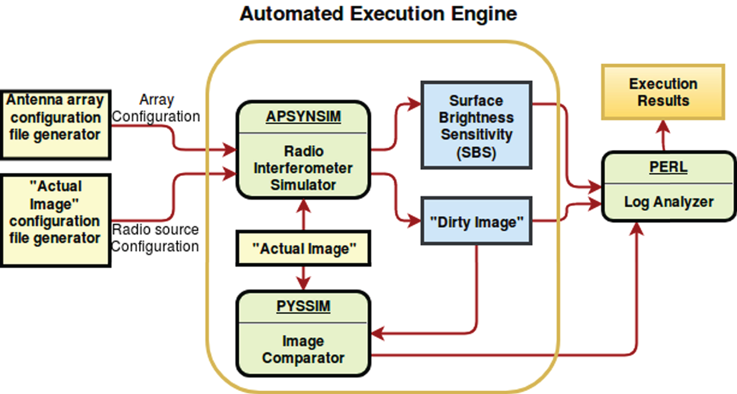
Framework used for automated generation of observed images and subsequent data analysis.

The performance evaluation metrics, namely, SSIM and Surface brightness sensitivity (SBS) used to evaluate the imaging performance of antenna arrays has been explained below. The measure of similarity, SSIM, between two images, the “actual image” - I and the “dirty image” - I_D is given by Equation (6) [30]. $SSIM (I, I_{D}) = lum (I, I_{D}) cont (I, I_{D}) sim (I, I_{D})$ (6) $lum (I, I_{D}) = \frac{2 μ_{I} μ_{I_{D}} + C_{1}}{μ_{I}^{2} + μ_{I_{D}}^{2} + C_{1}}$ (7) $cont (I, I_{D}) = \frac{2 σ_{I} σ_{I_{D}} + C_{2}}{σ_{I}^{2} + σ_{I_{D}}^{2} + C_{2}}$ (8) $sim (I, I_{D}) = \frac{σ_{{II}_{D}} + C_{3}}{σ_{I} σ_{I_{D}} + C_{3}}$ (9) where lum (I, I_D), cont (I, I_D) and sim (I, I_D) are luminance, contrast and structure comparison function respectively.

The closeness of mean(μ) luminance of “actual image” and “dirty image” is given by Equation (7) [30]. Contrast closeness, using standard deviation(σ), of the two images is given Equation (8) [30]. The correlation coefficient of the two images and a measure of their similarity is provided by Equation (9) [30]. In Equation (9) σ_{II_D} is the covariance of two images. C₁, C₂ and C₃ are arbitrary constants. SSIM ranges between zero and one. A value of one indicates that the two images are identical, while a value of zero implies that the two images have no similarity at al. Pyssim module, a python library was employed for image comparison using SSIM metric [31].

The sensitivity of an antenna array to a point source can be very much different than the sensitivity of the antenna array to extended sources [19]. SBS [19](Jy/beam) is the metric used for evaluating the sensitivity of the antenna array to extended sources. SBS, I_f, is given by Equation (10)-Eq. (13) [19, 32]. APSYNSIM was employed to compute the SBS.

$I_{f} = \frac{2 {hf}^{3}}{c^{2}} \frac{1}{e^{\frac{hf}{{kT}_{bmin}}}}$ (10) where h is Planck’s constant, c is the velocity of light in vacuum and T_bmin is the minimum brightness temperature.

$T_{bmin} = \frac{2 \log_{e} (2)}{π} \frac{c^{2}}{k} \frac{Δ I}{f^{2} θ_{hpbw - sba}^{2}}$ (11) where ΔI is the image sensitivity and θ_hpbw-sba is the half power beam width of synthesized beam.

$Δ I = \frac{SEFD}{\sqrt{2} η_{B} \sqrt{(N) (N - 1) Δ f t_{int}}}$ (12) where SEFD is the System Equivalent Flux Density, N is the number of antenna in the antenna array. η_B is system efficiency and t_int is the integration time.

$SEFD = \frac{2 {kT}_{sys}}{η_{A} A_{ant}}$ (13) where T_sys is noise temperature, η_A is antenna efficiency and A_ant is antenna area.

6 Results and discussions

Proof of log-periodic antenna array as an optimal solution to the “configuration problem” is obtained. Results of the maximization of radio imaging performance of a log-periodic spiral antenna array have been presented. Further, the performance-optimized spiral antenna array and the perfect Y antenna array have been evaluated for frequency response, integration time, and angular resolution. The results obtained, along with a comprehensive analysis, has been presented in this section.

6.1 Log periodic antenna array: An optimal solution

In this section, we prove that the log-periodic spiral antenna array is an optimal solution to the “configuration problem”. As discussed in Sect. 3, according to Chow, an optimum solution is achieved when the radial distance of the antenna elements, r in an antenna array configuration, is inversely proportional to 3D track density, which is in-turn inversely proportional to 2D baseline density (Equation (2)).

It can be deduced further that 2D baseline density is proportional to the element surface density (number of differential antenna element per elemental surface area) and is given by Equation (14), where rdθdr is the elemental surface area of the spatial plane.

$2 D baseline density \propto \frac{d n (r, θ)}{r d θ d r}$ (14)

A two step process is adopted to solve Equation (14). In Step I, r is kept fixed at a constant value say r₀ and the variation of n^th antenna element with respect to θ is investigated. In this case Equation (14) can be rewritten as follows.

$\begin{matrix} 2 D baseline density \propto \frac{\partial n (θ)}{r_{0} \partial θ} \\ But r \propto \frac{1}{2 D baseline density} \\ \Rightarrow \frac{\partial n (θ)}{r_{0} \partial θ} = l_{1} \frac{1}{r_{0}} \\ \Rightarrow \partial n (θ) = l_{1} \partial θ \end{matrix}$

Integrating both sides, Equation (15) is obtained. $n (θ) = l_{1} θ$ (15)

In Equation (15), l₁ is a proportionality constant. From Equation (15), it can be inferred that for optimum performance, antennas are required to be equiangular spaced. For example, if first antenna (n=1) is placed at 30°, second antenna (n=2) has to be placed at 60° and so on such that the ratio n/θ is a constant.

In Step II, θ is kept fixed at a constant value say θ₀ and variation of n^th antenna element with respect to r is studied. For this scenario, Equation(14) can be rewritten as follows. In Equation (16), l₂ and l₃ are proportionality constants.

$\begin{matrix} 2 D baseline density \propto \frac{\partial n (r)}{\partial r} \\ But r \propto \frac{1}{2 D baseline density} \\ \Rightarrow r = l_{2} . \frac{1}{(\frac{\partial n (r)}{\partial r})} \\ \Rightarrow \frac{\partial r}{r} = l_{3} \partial n (r) \end{matrix}$

Integrating both sides, ln (r) = l₃ (n (r))

$\Rightarrow r = e^{l_{3} n (r)}$ (16)

The locus traced out by a log-periodic spiral is represented by Equation (15) and Equation (16), and hence it can be inferred that a log-periodic spiral antenna array configuration is an optimum solution to the “configuration problem”.

6.2 Maximizing spiral antenna array imaging performance

The variation of SSIM as a function of the spacing between successive antenna elements with a distinct innermost spiral radius is shown in Fig. 5. The configuration parameters are listed in Table 1. From Fig. 5, it is evident that for angles between 50° and about 150°, SSIM is the largest for a spiral antenna array with the inner radius equal to 0.1 units. Also, it can be seen that at 120°, there is a peak, irrespective of the inner radius of the antenna array. Hence, to obtain the most efficient imaging performance, a spiral antenna array with an inner radius of 0.1 units and the angular spacing between adjacent antenna elements set to 120° is required for an antenna array with a radius of 20 units.

Fig. 5

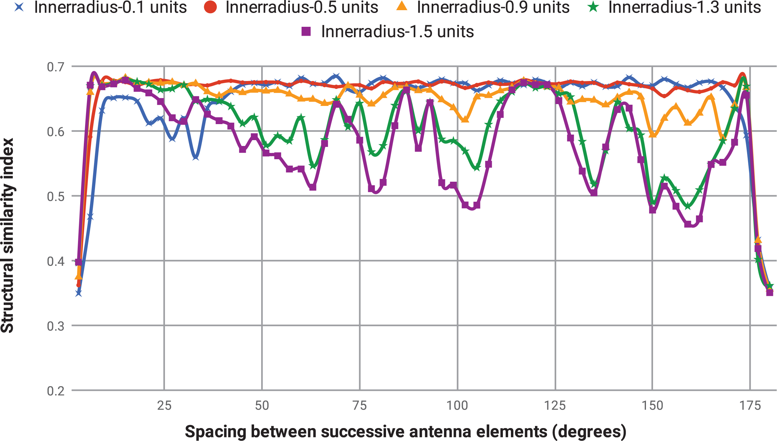
Design of log periodic spiral antenna array. Optimal performance for the spiral antenna array with outermost radius 20 units is achieved when innermost spiral radius is 0.1 units and angular spacing is 120°.

6.3 Frequency response

Frequency response influences the accuracy of a radio interferometer. The smearing of detail occurs in the outer regions of the re-created radio image, which in turn limits the field of view of the radio interferometer. The amount of smearing depends on the nature of the passband of frequency response. Smearing is the least for a rectangular passband. Frequency response also affects the sensitivity of the instrument, thus determining the quality of imaging. The sensitivity of the instrument is proportional to the Signal to Noise Ratio (SNR) of the instrument. SNR of a radiometer is given by Equation (17) [33] and is a measure of sensitivity of the instrument. In Equation (17), β is the width of the passband, τ_i is the integration time and k is the proportionality constant.

$η = k (β τ_{i})^{1 / 2}$ (17)

From Equation (17), it is evident that for greater sensitivity frequency response with a rectangular passband with a wide width is desired. Also, a typical radio source emits a continuum of frequencies without any sharp spectral lines. Hence a rectangular passband frequency response with wide bandwidth is desired.

Further, in the scenario of earth imaging from satellite using interferometry, the bandwidth is severely limited by radio frequency interference (RFI). Hence a high bandwidth offers large tolerance at hand to offset effects due to RFI.

The comparison of frequency response for the spiral antenna array and the perfect Y array using the SSIM metric is shown in Fig. 6(a)-(b). For each antenna array, the frequency response obtained for space imaging from the earth and earth imaging from space are plotted. Antenna dimensions, namely, antenna array radius and antenna radius, used for space imaging from the earth are about a few thousands of times larger than the ones used for earth imaging from space. The exact dimensions used are indicated in Table 1. However, from Fig. 6(a)-(b), it is evident that the frequency response for earth imaging and space imaging for an antenna array follow a similar trend.

Fig. 6

Comparison of frequency response for the antenna arrays using SSIM metric. Space imaging and earth imaging frequency response follow a similar trend. The average bandwidth of spiral antenna array is about five times that of perfect Y antenna array.

The spiral antenna array has the desired rectangular response. Further, the spiral antenna array has a wider bandwidth, resulting in a higher degree of accuracy in measurement, with less smearing of details at the image boundaries. Using a target SSIM of 0.6, the average bandwidth of spiral antenna array is 9.6 GHz, while that of the perfect Y antenna array is only 1.9 GHz, a difference of a factor of about five. Hence, the ratio of sensitivities for given integration time, as per Equation (17), is (9.6/1.9) ^0.5 = 2.23. The spiral antenna array configuration has about 2.23 times higher sensitivity (or SNR) than the perfect Y antenna array; hence, it is capable of producing higher quality images.

As already mentioned, the SBS metric (Fig. 7(a)-(b)) signifies the lower threshold of the radio-telescope in resolving a faint image. At higher frequencies, specifically above 10 GHz, the spiral antenna array offers a better SBS compared to the perfect Y antenna array. However, at lower frequencies below 3 GHz, perfect Y antenna array outperforms, but only marginally, the spiral antenna array concerning SBS metric. Between 3 and 10 GHz, the SBS frequency response is similar for both the spiral antenna array and the perfect Y antenna array. We can conclude that the spiral antenna array offers better SBS for much higher bandwidth of 50 GHz (10 to 60 GHz) than the perfect Y antenna array (<3 GHz).

Fig. 7

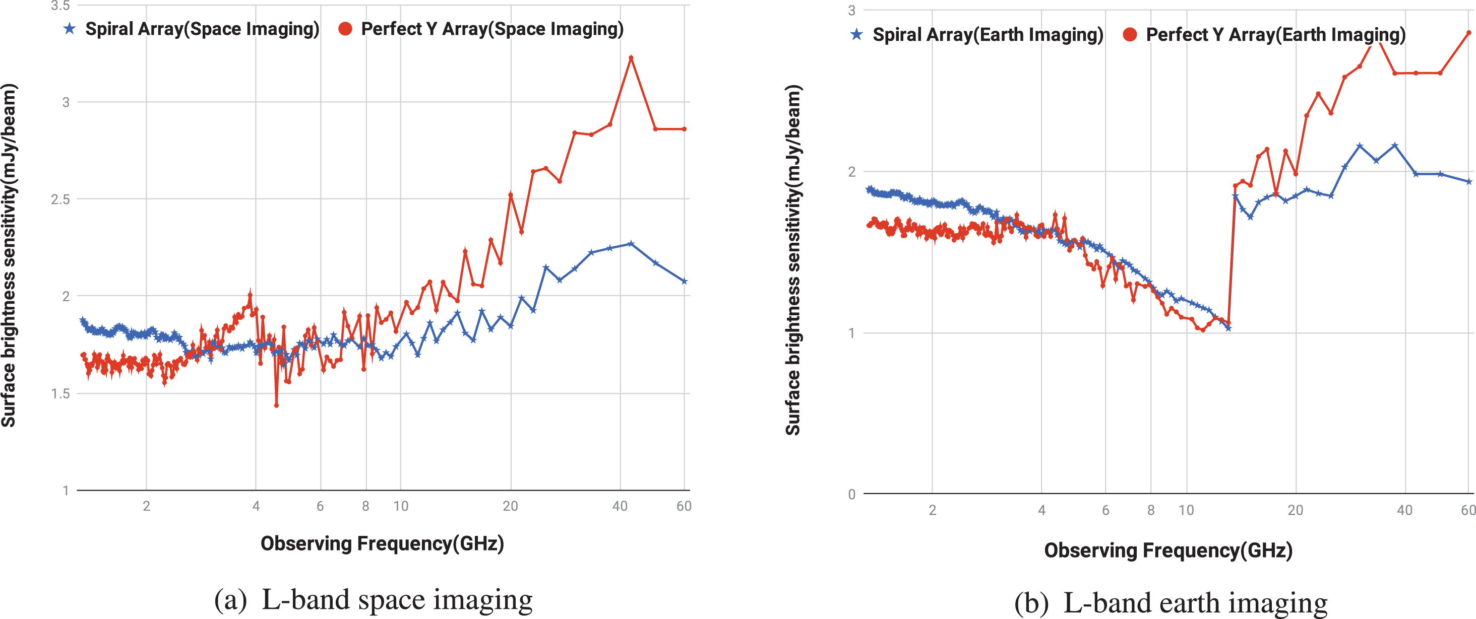
Comparison of frequency response for the antenna arrays using SBS metric. Above 10 GHz spiral antenna array offers better SBS. Below 3 GHz perfect Y antenna array excels spiral antenna array.

6.4 Integration time

A filled antenna array configuration can work on a “snapshot mode”, with almost negligible integration time. On the other hand, sparse antenna arrays such as the perfect Y configuration and the spiral configuration requires non zero integration time to produce high-resolution images equivalent to a filled antenna array.

The integration time depends on Fill factor, F which is given by Equation (18) [34]. In Equation (18) M is the number of antennas in the array, d is the antenna diameter, and D is the diameter of the array occupied area.

$F = \frac{{Md}^{2}}{D^{2}}$ (18)

A decrease in F will necessitate an increase in integration time to maintain the same image quality. Similarly, a shorter integration time will force F to be increased to secure the same image quality. The dependency of change in F with change in integration time factor, Δt_int is given by Equation (19) [35]. Δt_int is the ratio of integration times of two different array topologies.

$Δ t_{int} \propto \frac{1}{(Δ F)^{3}}$ (19) Since F is dependent on M, d or D as given in Equation (18), a change in Δt_int, can impact M, d and D.

The integration time is varied from 0.2 hours to 9 hours, in steps of 0.1 hours with the other parameters, shown in Table 1 kept fixed. SSIM and SBS are measured for the spiral antenna array and the perfect Y antenna array for both space and earth imaging. The results are plotted and shown in Fig. 8(a)-(b) and Fig. 9(a)-(b) respectively. From Fig. 8(a)-(b), it is seen that to achieve an image quality of SSIM of more than 0.6, the spiral antenna array will need only about 1.5 hours while a perfect Y antenna array will need about 3 hours, a difference of a factor of two.

Fig. 8

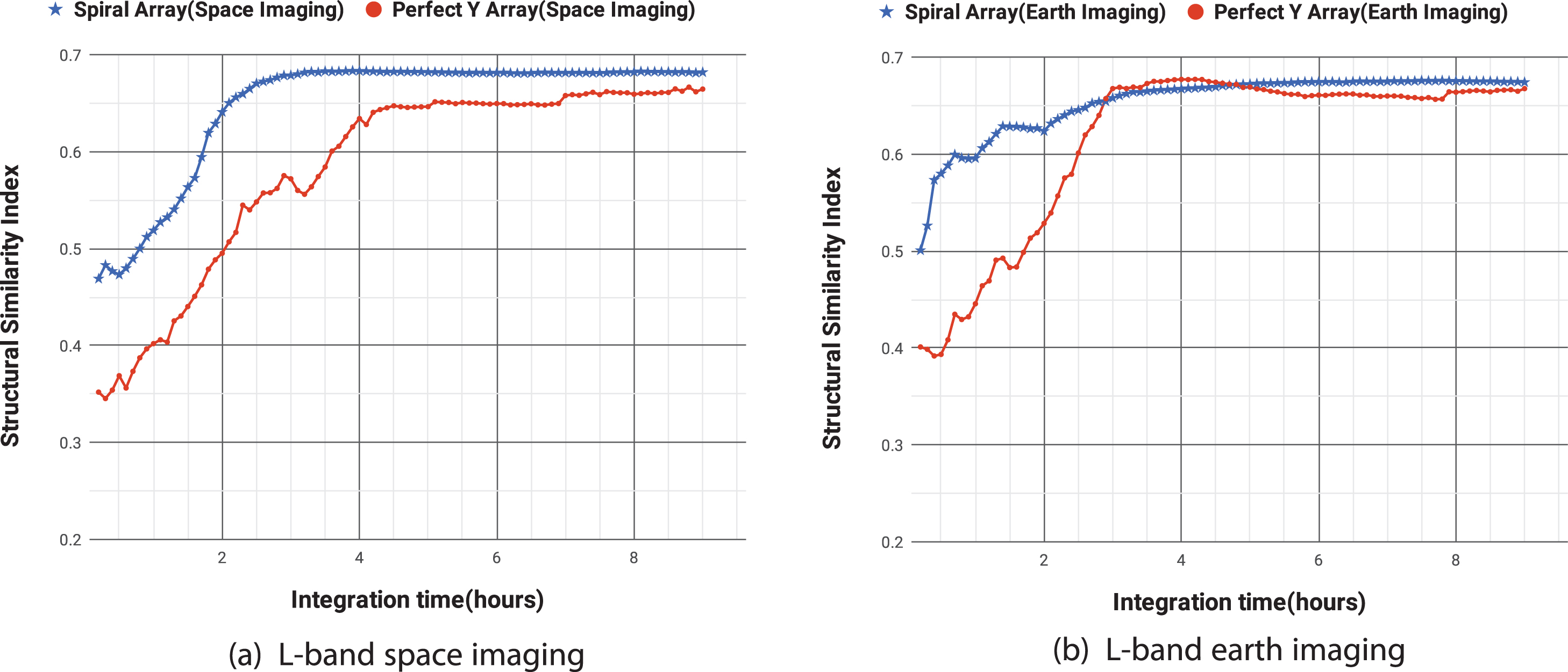
Comparison of integration time response for the antenna arrays using SSIM metric. The spiral antenna arrays have a faster integration time than the perfect Y antenna array leading to a decrease in required number of antennas and an increase in field of view.

Fig. 9

Comparison of integration time response for the antenna arrays using SBS metric. For a shorter integration time, the spiral antenna array offers a better SBS, while the perfect Y antenna array has a better SBS for a longer integration time.

With Δt_int = 2, using Equation (19), $Δ F \propto 1 / Δ t_{int}^{3}$ = 0.125 is obtained. Since the spiral antenna array has a faster integration time, its fill factor can go down by 12.5% and can still have the same performance as that of the perfect Y antenna array. It is desired to examine how this relaxation in fill factor, can help to reduce the number of antennas or antenna dimension in the case of space imaging. Since Δt_int > 1 for earth imaging scenario, the advantages realized by the spiral antenna array for space imaging case is applicable for earth imaging also.

F of perfect Y antenna array, using Equation (18) gives F_perfectY = (1.054) .10^-5. With a 12.5% tolerance, the fill factor of the spiral antenna array is computed by using Equation (20)-Equation (21). $F_{spiral} = F_{perfectY} - (12.5 %) . F_{perfectY}$ (20) $\Rightarrow \frac{F_{spiral}}{F_{perfectY}} = 0.875$ (21) Using Equation (18), Equation (20) number of antennas required by spiral configuration, M_spiral = 23.64. Hence equivalent spiral antenna array can have three antennas less (about 10% reduction) with d and D remaining unchanged. Similarly, antenna diameter employed by spiral configuration, d_spiral = 23.38 m. Thus an equivalent spiral antenna array used for space imaging can employ a smaller antenna with M and D remaining unchanged. A smaller antenna in turn results in a wider instantaneous field of view, Δφ as given by Equation (22) [36]. The wider field of view facilitates the imaging of larger regions of the sky. Array diameter employed by spiral configuration can be extended to D_spiral = 42.4km, which in turn improves the angular resolution, as it will be seen later. However, this comes at the price of increased infrastructure. In Equation (22), λ is the operating wavelength, d_ant is the antenna diameter. $Δ φ = \frac{1.02 λ}{d_{ant}}$ (22)

It can be seen from Fig. 9(a)-(b) that SBS for the spiral antenna array is better than the perfect Y antenna array for a shorter integration time of up to 2.25 hours. For longer integration time beyond 2.25 hours, the perfect Y antenna array offers a better SBS. Further, it is noted that SBS gets better with an increase in integration time but reaches a saturation point as expected. This could be attributed to the rise of redundant uv-tracks with an increase in integration time.

6.5 Angular resolution

The capability to distinguish two closely placed identical point sources is the angular resolution. An excellent resolution is required to capture finer details of a radio source. For example, the achievable resolution at RF frequency spectrum limits the detection of exoplanets using radio-telescopes [37]. This limitation is in contrast to optical telescopes [38], which has been able to discover exoplanets. Thus the quest continues for improving the angular resolution of radio telescopes.

Angular resolution is given by Equation (23) [36]. In Equation (23), λ is the operating wavelength and B_max is the maximum operating baseline. It is seen from Equation (23), that the angular resolution is a function of observing frequency and the longest baseline length, which in turn can be obtained by increasing radial periphery of the antenna array, D. Using the values given in Table 1 and using B_max = 25 km (for perfect Y antenna array), Δθ is 15.9 milli-arcsecond for the perfect Y antenna array.

$Δ θ = \frac{1.02 λ}{B_{\max}}$ (23)

With the configuration parameters, as shown in Table 1, the source model size is increased in steps of 6 arc seconds while keeping the image layout constant, thereby increasing angular resolution in steps of 12.5 milli-arc seconds. The SSIM for the image processed by both spiral and perfect Y are obtained and plotted in Fig. 10. The best resolution that is obtained for the perfect Y antenna array is 150 milli-arcsecond. Further, as the angular resolution is deteriorated by increasing its value, the image quality degrades as expected. However, the degradation is rapid for a perfect Y antenna array while it is gradual for the spiral antenna array. From the figure, it can be inferred that for the desired SSIM of 0.6, angular resolution can be increased up to 1.5 arc-sec for spiral, but for perfect Y antenna array, it can be increased only up to 315 milli-arc seconds, a factor of about five. Thus for a given configuration, it can be seen that a spiral antenna array configuration can resolve an image that is five times smaller. The resolving ability can also be regarded as a magnification ability of the spiral antenna array over the perfect Y antenna array. A spiral antenna array has a magnification capability of 5x compared to an equivalent spiral antenna array. However, for sub 100 milli-arcsecond resolution, the perfect Y antenna array has better imaging performance.

Fig. 10

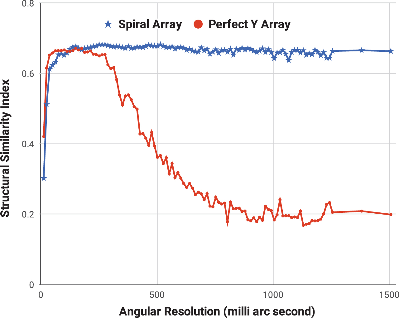
Comparison of angular resolution for the antenna arrays. Spiral antenna array can resolve an image that is five times smaller compared to a perfect Y antenna array.

7 Conclusions

The imaging performance evaluation has been carried out in the image-plane using two metrics, namely SSIM and SBS. While SSIM provides an objective measure of the quality of the observed image for the reference test image, SBS is a figure of merit used to quantify the ability of the antenna array to reliably detect faint images (images that have very low surface brightness). The frequency response, integration time response, and angular resolution are the imaging performance evaluation parameters.

A random image with a Gaussian distribution was used as a reference test radio source. APSYNSIM, a radio interferometer simulator, used the test radio source to simulate the observation. The observation consisted of 1740 “dirty images” generated by both the log-periodic spiral antenna array and the perfect Y antenna array.

It was found by simulation that for an L-band spiral antenna array with an outer radius of 20 units, the best imaging performance is obtained when certain conditions are satisfied. These conditions are (i) the angular spacing between adjacent antenna elements along the spiral trajectory is 120° and (ii) the inner radius of the spiral is 0.1 units. The imaging performance of the L-band log-periodic spiral antenna array has been compared with the perfect Y antenna array.

The L-band log-periodic spiral antenna array has outperformed the perfect Y configuration in most of the imaging performance evaluation aspects. The spiral antenna array has the desired rectangular frequency response with wide bandwidth. The spiral antenna array has a higher SNR and a larger field of view. The angular resolution is better than the perfect Y array.

Despite numerous advantages, there are a few shortcomings of the L-band log-periodic spiral antenna array. Perfect Y antenna array has a better SBS at a low observing frequency of up to 3 GHz. This implies that an L-band log-periodic spiral antenna array has a slightly inferior SBS than an equivalent perfect Y antenna array. For longer integration time beyond 2.25 hours, the perfect Y antenna array offers a better SBS. For sub 100 mill-arc second resolution, an equivalent perfect Y antenna array has a higher SSIM compared to L-band log-periodic antenna array.

It can be concluded that the log-periodic spiral antenna array is an optimum antenna array configuration. Further, the L-band log periodic antenna array has a better radio-imaging performance compared to an equivalent perfect Y antenna array.

The existing earth-observation radio interferometric imaging systems operate in the L-band. Hence, the performance of the antenna array has been assessed in the L-band and the results obtained. However, the radio interferometric concept applied to radio astronomy, cannot be applied directly for earth observations. Though similar, they are not identical. Enhancement of APSYNSIM to enable simulations specifically for earth observations is required. More accurate imaging performance of the spiral antenna array specifically for the earth observation is a topic of future study.

References

Corbella

, Torres

, Duffo

and Martín-Neira

, Interferometric radiometry measurement concept: The visibility equation, in: Geoscience and Remote Sensing Symposium (IGARSS), 2011 IEEE International, IEEE, (2011), pp. 3491–3494.

Rajendran

and Shanmugha Sundaram

G.A.

, Phased antenna array design for l-band aerospace detection of radiolytic component, Proceedings of 11th SPCOM, IEEE Inc. (2016), pp. 81.

Rajendran

and Shanmugha Sundaram

G.A.

, Design and evaluation of printed log periodic dipole antenna for detection of radiolytic components, Proceedings of 11th ICCSP, IEEE Inc. (2016), 32.

Rajendran

and Shanmugha Sundaram

G.A.

, Design and evaluation of printed log periodic dipole antenna for an L band electrically steerable array system, Proceedings of 1st ICCSC, IEEE Inc. (2014), 311.

Ratheesh

K.M.

, Seah

L.K.

and Murukeshan

V.M.

, Spectral phase-based automatic calibration scheme for swept source-based optical coherence tomography systems, Physics in Medicine and Biology61(21) (2016), 7652–7663.

Meleppat

R.K.

, Shearwood

, Seah

L.K.

and Matham

M.V.

, Quantitative optical coherence microscopy for the in situ investigation of the biofilm, Journal of Biomedical Optics21(12) (2016), 1–9, 9.

Ratheesh

K.M.

, et al, Gold nanorods with higher aspect ratio as potential contrast agent in optical coherence tomography and for photothermal applications around nm imaging window, Biomedical Physics & Engineering Express2(5) (2016), 055005.

Boone

, Interferometric array design: Optimizing the locations of the antenna pads, Astronomy & Astrophysics377(1) (2001), 368–376.

Chow

, On designing a supersynthesis antenna array, IEEE Transactions on Antennas and Propagation20(1) (1972), 30–35.

10.

Shanmugha Sundaram

G.A.

and Subramanian

K.R.

, Spectrum of solar type I continuum noise storm in the 50–80 MHz band and plasma characteristics in the associated source region, Astrophysical Journal605(2) (2004), 948.

11.

Conway

, Self-similar spiral geometries for the LSA/MMA, ALMA Memo Series (1998), 216.

12.

Jones

, Geometric configuration constraints for large deep space network arrays,, The Interplanetary Network Progress Report42 (2004), 157.

13.

Lal

D.V.

, Lobanov

A.P.

and Jiménez-Monferrer

, Array configuration studies for the Square Kilometre Array-Implementation of figures ofmerit based on spatial dynamic range, arXiv preprint arXiv:1001.1477 (2010).

14.

Holdaway

and Helfer

T.T.

, Interferometric array design, in: Synthesis Imaging in Radio Astronomy II, 180 (1999), p. 537.

15.

Zhang

, Wang

and Lin

, Interferometric array assessment: Investigating UV coverage and imaging, in: Image and Signal Processing (CISP), 2011 4th International Congress on, 3 IEEE, (2011), pp. 1577–1583.

16.

Wang

, Bovik

A.C.

, Sheikh

H.R.

and Simoncelli

E.P.

, Image quality assessment: from error visibility to structural similarity, IEEE Transactions on Image Processing13(4) (2004), 600–612.

17.

Steger

, Ulrich

and Wiedemann

, Machine vision algorithms and applications, John Wiley & Sons2018 (2018).

18.

Maddikonda

S.S.

and Shanmugha Sundaram

G.A.

, Proceedings of 3rd ICCSP, IEEE Inc. (2014), 866.

19.

Perley

R.A.

, Schwab

F.R.

and Bridle

A.H.

, Synthesis imaging in radio astronomy, in: Synthesis Imaging in Radio Astronomy6 (1989), 1989.

20.

Martin-Neira

, Goutoule

J.-M.

, Knight

, Claude

, Bara

, Camps

, Torres

, Corbella

, Lannes

, Anterrieu

, et al., Integration of MIRAS breadboard and future activities, in: Geoscience andRemote Sensing Symposium, 1996. IGARSS’96.’Remote Sensing for a Sustainable Future.’, International, 2 IEEE, (1996), pp. 869–871.

21.

Chow

, Comparison of some correlation array configurations for radio astronomy, IEEE Transactions on Antennas and Propagation18(4) (1970), 567–569.

22.

Keto

, The shapes of cross-correlation interferometers, The Astrophysical Journal475(2) (1997), 843.

23.

Kogan

, Optimization of an array configuration minimizing side lobes, MMA Memo171 (1997).

24.

Holdaway

, Foster

S.M.

and Morita

, Fitting a 12km configuration on the chajnantor site, Tech rep MMA Memo153 (1996).

25.

Martán-Neira

, LeVine

, Kerr

, Skou

, Peichl

, Camps

, Corbella

, Hallikainen

, Font

, Wu

, et al, Microwave interferometric radiometry in remote sensing: An invited historical review, Radio Science49(6) (2014), 415–449.

26.

Sundar

and Shanmugha

G.A.

, Simulated optimal logspiral topologies for the square kilometer array, in: Proceedings of the 2014 International Conference on Interdisciplinary Advances in Applied Computing, ACM, (2014), p. 4.

27.

Weiman

C.F.

and Chaikin

, Logarithmic spiral grids for image processing and display, Computer Graphics and Image Processing11(3) (1979), 197–226.

28.

Marti-Vidal

, APSYNSIM: An Interactive Tool to Learn Interferometry, arXiv preprint arXiv:1706.00936 (2017).

29.

Antoine Vacavant

C.G.

and Terrace

, A Python module for computing the Structural Similarity Image Metric (SSIM) (2019).

30.

Hore

and Ziou

, Image quality metrics: PSNR vs. SSIM, in: Pattern recognition (icpr), 2010 20th International Conference on, IEEE, 2010 (2010), pp. 2366–2369.

31.

Wang

, Bovick

, Sheikh

and Simoncelli

, The SSIM Index for Image Quality Assessment, Matlab Implementation (2010).

32.

Wrobel

and Walker

, Synthesis Imaging in Radio Astronomy II, in: Sensitivity, ASP Conference Series, 180 (1999), pp. 171–186.

33.

Thompson

and d’Addario

, Frequency response of a synthesis array: Performance limitations and design tolerances, Radio Science17(2) (1982), 357–369.

34.

Liu

, Jiang

, Wang

and He

, Novel array configuration and its optimization for sparse aperture imaging systems, Optical Engineering50(5) (2011), 053202.

35.

Fienup

J.R.

, MTF and integration time versus fill factor for sparse-aperture imaging systems, in: Imaging Technology and Telescopes, International Society for Optics and Photonics, 4091 (2000), pp. 43–48.

36.

Monnier

J.D.

and Allen

R.J.

, Radio and optical interferometry: Basic observing techniques and data analysis, in: Planets, Stars and Stellar Systems Springer (2013), pp. 325–373.

37.

Siemion

A.P.

, Demorest

, Korpela

, Maddalena

R.J.

, Werthimer

, Cobb

, Howard

A. W.

, Langston

, Lebofsky

, Marcy

G.W.

, et al, A 1.1–1.9 GHz SETI survey of the Kepler field. I. A Search for narrow-band emission from select targets, The Astrophysical Journal767(1) (2013), 94.

38.

Labeyrie

, Resolved imaging of extra-solar planets with future 10–100km optical interferometric arrays, Astronomy and Astrophysics Supplement Series118(3) (1996), 517–524.