Intelligent autonomous navigation system for UAV in randomly changing environmental conditions

1 Introduction

The safe and reliable navigation of such autonomous systems as unmanned aerial vehicles (UAV) is a complex open problem in robotics, where a robotic system must simultaneously do many tasks of perception, control and localization. This task is especially complicated when working in an uncontrolled, unpredictable environment, for example, on city streets, in wooded areas, etc. In these cases, the autonomous agent must not only be guided to avoid collisions, but also interact safely with other agents in the environment.

The traditional approach to solving this problem is a two-stage process with alternation, consisting of automatic localization on a given map using GLONAS/GPS, sensors and calculation of control commands, so that the agent can avoid obstacles when reaching its goal [1, 2]. Despite the fact that modern mapping and localization algorithms provide localization in a wide range of conditions [3], visual overlay, dynamic scenes, and strong changes in appearance can lead a perception system to fatal errors. In addition, the separation of the perception and control units not only prevents any possibility of positive backward linkage between them, but also creates a complex problem of determining control commands from three-dimensional maps.

2 Mapping-localization-planning

An unmanned aerial vehicle is usually equipped with GPS and a computer vision system for assessing the status of the system, warning about the obstacles, and performing route planning [1, 2]. Nevertheless, these systems are still prone to failures in the presence of a weak GPS signal, which is observed, for example, on city streets or in wooded areas. In addition, it is still not clear how to identify and avoid the static and dynamic obstacles that are present in these conditions. A common approach in GPS scenarios is mapping-localization-planning, where the robot simultaneously builds a map of the environment and independently localizes in it [5–7]. However, these approaches may fail to localize on a map that was created under significantly different conditions or during periods of high acceleration (due to motion blur and loss of object tracking). In addition, ensuring global consistency leads to greater computational complexity and significant difficulties in working with dynamic environments. Indeed, SLAM methods only allow navigation in a “predominantly static world”, where waypoints and (optionally) collision-free trajectories can be statically determined.

3 Justification of the choice of neural network methods

A complex environment, first of all, means such properties of the space around the robot, which make it difficult to recognize possible routes. For example, forest glades, various trails and other paths in the forest.

To solve the problems of autonomous navigation in such conditions, it is proposed to use the classification and decision-making methods implemented using artificial neural networks. Studies show that using the deep parallelization method of calculations is a promising way to solve the problems of increasing the intelligence and autonomy of mobile robotic objects, which, in turn, requires the development of specialized hardware platforms that provide maximum efficiency for the implementation of these algorithms and methods.

4 Development of the appearance of an autonomous navigation system

The autonomous navigation system under development is intended for use in mobile systems that move in complex, randomly changing and unpredictable conditions, i.e. in dynamically changing conditions of a wooded area, which imposes restrictions on the speed of work and the quality of laying the route.

The functional diagram of the developed system is presented in Fig. 1.

OPEN IN VIEWER

Fig. 1

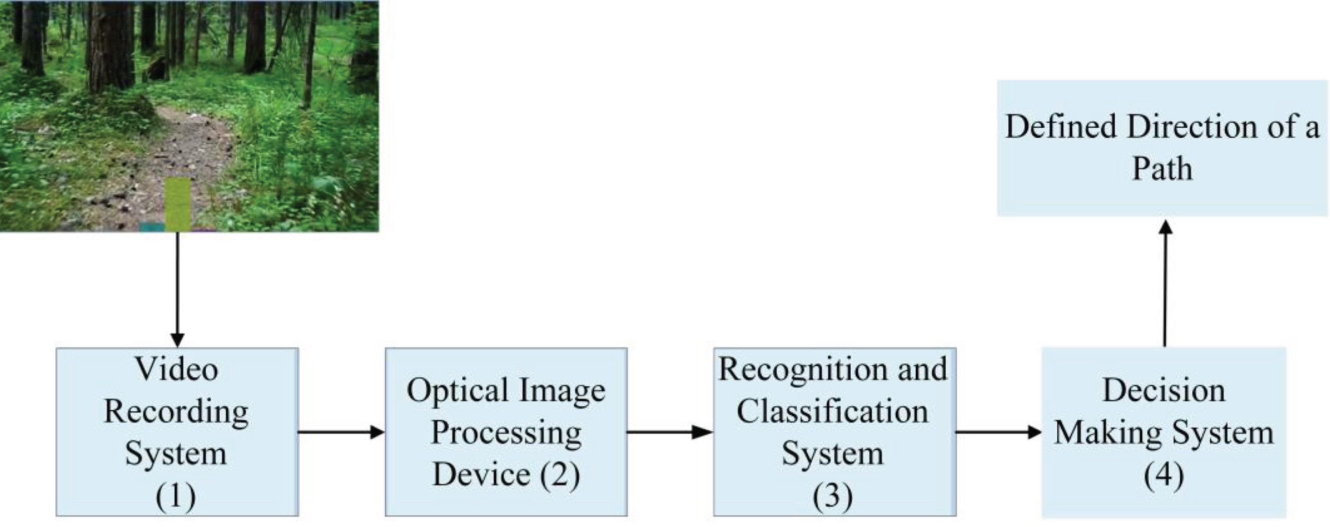
Functional diagram of the system under development.

Unit (1) consists of an optical system, CMOS or CCD matrices, which converts the analog image signal into a digital signal. Preliminary studies have shown that for effective navigation, the system’s field of view should be at least 120 horizontally.

System unit (2) digitally processes the signals coming from system (1) and transmits the processing results to the input of system (3). The main function of system (2) is to extract the information necessary for recognition and classification efficiency of system (3) from the optical image obtained by system (1).

System (3) is a classifier, which is an artificial neural network of deep learning of direct propagation with a complex configuration, trained to recognize passable routes on the video image obtained by system (1). The structure of system (3) has the form of a map of network layers. Since an RGB image is fed to the network input, unit (3.1) is a layer consisting of 3 two-dimensional arrays of size MxM neurons each, which together form the input network layer. The input layer is followed by hidden layers (3.2) –(3.M-3) with a decrease in the number of neurons in the layer in proportion to the movement to the output. The output layer of the network includes three neurons. The color-preserved input image is scaled anisotropically to the size M×M (at the current stage of research, M = 101) and enters the corresponding neuron matrix of the input layer. At the output of the network, there are three values reflecting the probability that the entrance belongs to the classes “path on the right”, “path on the left” and “path on the center”, respectively.

Unit (4) contains a decision making system and a path analysis system. The first is responsible for assessing and deciding on the direction of movement, the second is responsible for analyzing the incoming decision, based on information about previous trajectories, a map of the area, etc. Their work is interconnected, and the result is a set of motion control commands.

To develop the main module for classifying objects using neural networks, TensorFlow and Keras libraries with a programming interface for the Python language were chosen, because they provide a complete development cycle of neural network algorithms from experimental studies to integration into a real system. Also, they allow for fast development thanks to a convenient interface of Keras software. In Keras, a neural network is built as a sequence of standard library layers with specified parameters, i.e. the library provides a high level of abstraction. The usability of the selected libraries also lies in the fact that they allow saving to the hard disk and loading the entire trained neural network, the computational graph, and weights separately, which is convenient when using different sets of weights for the same architecture.

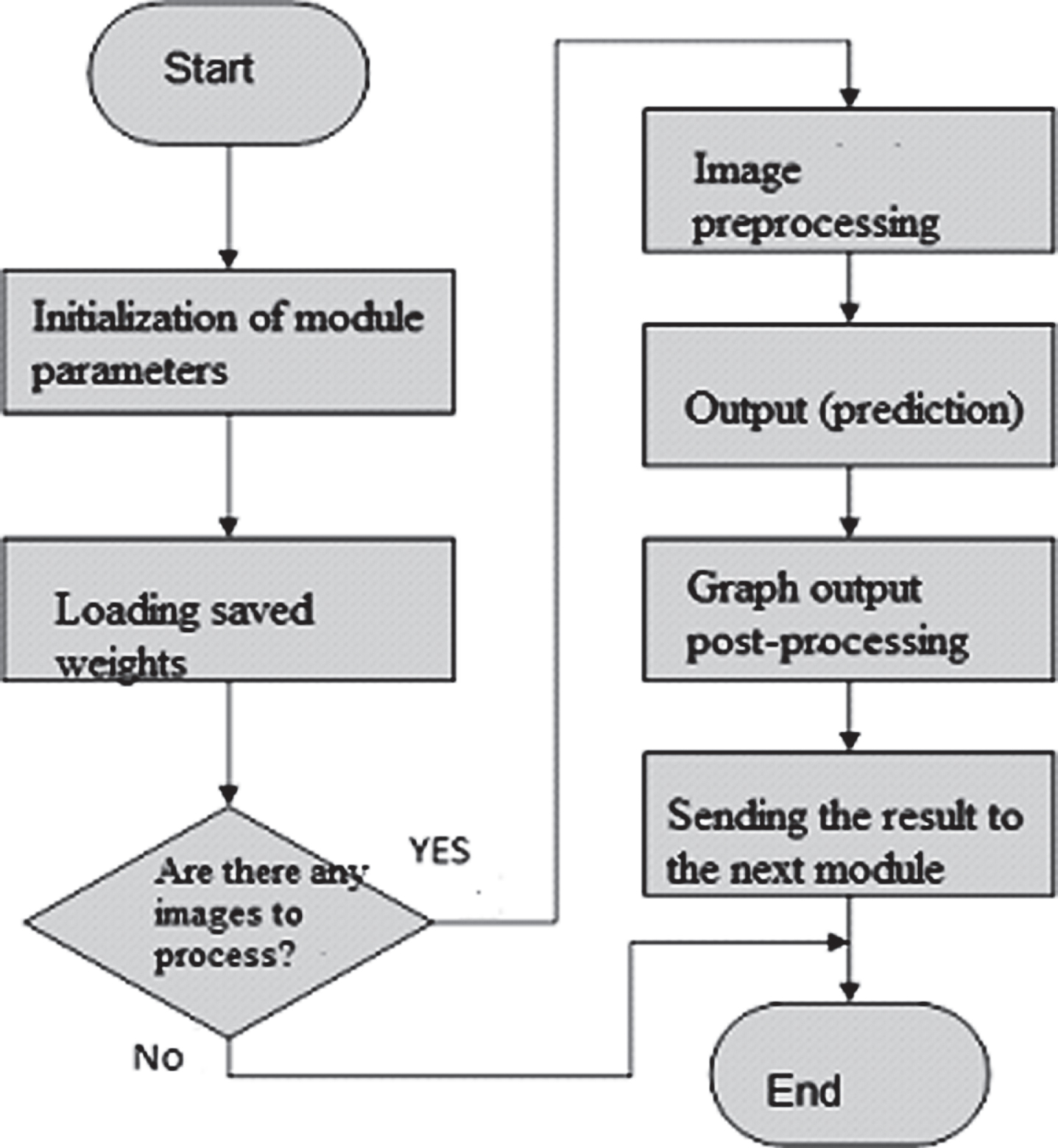
The function of the main object classification module is to define classes for all incoming images with given parameters. Its algorithm is shown in Fig. 2.

OPEN IN VIEWER

Fig. 2

Algorithm of the software module for image classification.

When starting the module, it is necessary to specify the module parameters:

- used neural network architecture (the module can work with various architectures);

- a file with weights (one architecture can be trained in several different ways, for example, in different classes);

- a list of class names (at the output of the network, there are only class identifiers in the form of numbers from 0 to N, N + 1 - the number of classes);

- the number of decimal places for the confidence value.

Then the module loads the specified architecture and the specified file with weights and waits for the image. When an image arrives, it is pre-processed if necessary - for example, resizing to fit the size of the input of the neural network, and then directly output, i.e. image processing by a neural network. At the output of the neural network, values are obtained which require post-processing to be converted to the target format - certain numerical transformations, as well as filtering by confidence value.

In addition to the main unit that uses the trained network to perform the classification, a unit is needed to perform training and testing operations of the network. Its need is determined not only at the stage of development of a neural network algorithm, but also at the stage of supporting computer vision system, in case a new set of annotated data appears and additional training is necessary. Also, if the appearance of the environment surrounding the mobile robot and other conditions change, it is advisable to re-assess the various trained models to select the most effective model in the new conditions.

The algorithm of such an auxiliary module shown in Figure 3 consists of several basic steps.

OPEN IN VIEWER

Fig. 3

Algorithm of the software module for training and assessment.

First, a dataset is created for training and testing with the given parameters - initial data for processing, a list of target classes, as well as augmentation parameters. Augmentation is a technique for increasing the amount of data used in machine training. To do this, copies of the original images are created, modified in some way, depending on the task. For example, brightness and contrast, dimensions and aspect ratio change, the image moves and rotates along different axes. Also, a set of basic values is calculated using the k-average method. The resulting data set is saved, and the algorithm proceeds to the training step. In this case, it is possible to set training hyperparameters: the number of training epochs, the size of the batch, the optimizer (the method of stochastic gradient descent - most often adaptive methods are used: Adam, RMSprop, Adagrad or Adadelta), the initial value of the training step.

The convolution neural network was trained on a data set consisting of 46,366 images. The test data set contains 10,490 images. The division was defined so that the appearance of the same section of the path in the training set and in the testing set was carefully avoided. Three classes were evenly represented in each set.

Python was chosen as a programming language, which in recent years has become a generally accepted language for many areas of application of data processing theory. It combines the power of programming languages with the ease of use of domain-specific scripting languages such as MATLAB or R. Python has libraries for loading data, visualizing, statistical computing, processing a natural language, image processing, and much more. This comprehensive toolkit offers data scientists an impressive arsenal of general and special tools.

When creating a convolutional neural network, the Keras add-in of the Tensorflow library was used for deep learning.

To create the model, training and test data are generated, located in folders with the names test_set and training_set.

The training_set folder contains three subfolders with images of the corresponding orientation, each of which contains about 15,000 images of the corresponding category. Images are a set of frames from the video of this passage along the forest paths filmed on video camera. The second folder “test_set” has a similar structure.

The process of building a convolutional neural network includes four main steps:

Step 1: Convolution

Step 2: Subsampling

Step 3: Smoothing

Step 4: Fully connected layer

The final architecture of the neural network is shown in Fig. 4. The total number of settable parameters was about half a million.

OPEN IN VIEWER

Fig. 4

Archietecture of a convolutional neural network in the Keras output window.

Below is a listing of the program of the main module of the classifier of RGB images based on a convolutional neural network.

As a result of the training, graphs of the predictive accuracy of the convolutional neural network and the loss function depending on the epoch of the neural network training were obtained, which are presented in Figs. 5 and 6.

OPEN IN VIEWER

Fig. 5

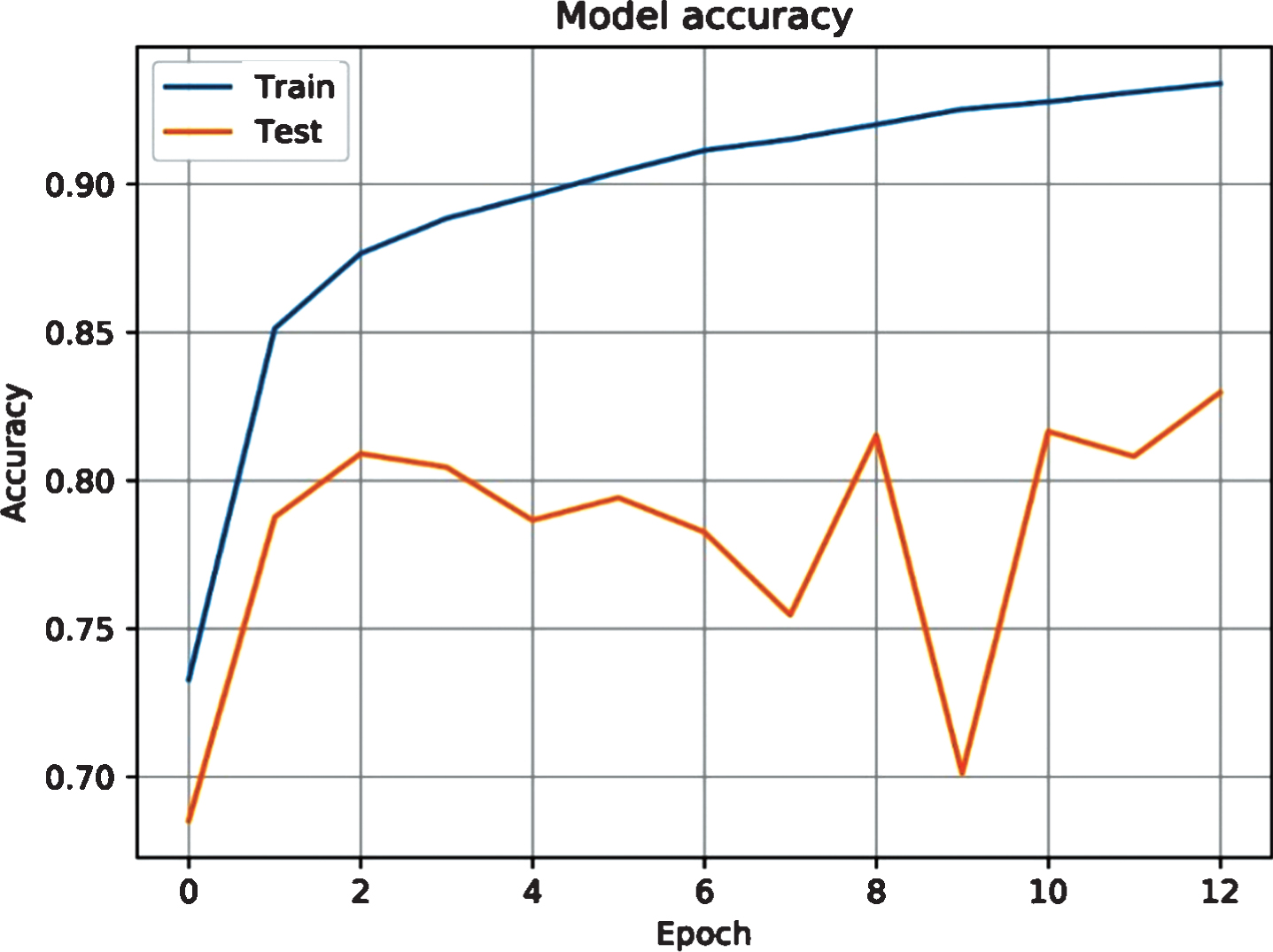
Model predictive accuracy.

OPEN IN VIEWER

Fig. 6

Example of video classification.

The difference in accuracy between training and testing indicates that the training data set does not have sufficient variability to make predictions for the test data set. However, the accuracy of predictions in the range of 80–85% can be considered acceptable for this type of task with a sufficient processing speed of frames received by the computer vision system of a mobile robot.

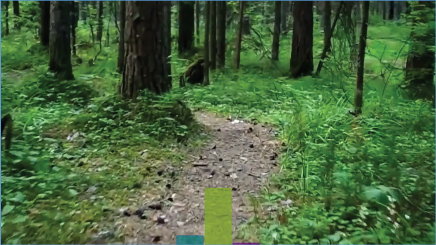
The result of the convolutional neural network operation is shown in Fig. 7.

At the output of the neural network, we get three numbers indicating the probabilities of belonging to one of the three classes: “path on the left” (TL), “path on the center” (GS) and “path on the right” (TR), which are presented in the form of a histogram (Fig. 7).

OPEN IN VIEWER

Fig. 7

Loss function.

The results of experiments conducted with a trained system in the field can be found in [8].

The developed system allows navigation of unmanned aerial vehicles in difficult environmental conditions. The results of training and the operation of the autonomous navigation system in the forest are presented. The system finds and follows the paths that are fairly difficult to distinguish. The results of field experiments are presented.

The disadvantages that should be eliminated include the high probability of taking wooden poles and trunks of some trees for the path. On the other hand, this problem is solved by the elementary use of additional computer vision systems. For example, the ultrasonic collision avoidance system that is used in most drones.

Further work in the field of the presented development will be aimed at expanding the capabilities for controlling the movement of the drone in a vertical plane.