
Abstract
The main objective of this research is to give an overview of the Analytic Hierarchy Process (AHP) in neutrosophic environment. In some realistic situations, the decision makers might be unable to assign deterministic evaluation values to the comparison judgments due to his/her limited knowledge or the differences of individual judgments in group decision making. To overcome these challenges, we have used neutrosophic set theory to handle the AHP, where each pair-wise comparison judgment is represented as a triangular neutrosophic number (TNN). In this paper, neutrosophic theory is used to form AHP decision-making model for choosing the best candidates among the applications. A real life example is developed based on expert opinions from Zagazig University, Egypt. The problem is solved to show the effectiveness of the proposed neutrosophic-AHP decision making model.
Keywords
Introduction
Multi-Criteria Decision Making (MCDM) is a formal and structured decision making methodology for dealing with complex problems [1]. Saaty [2] founded the Analytic Hierarchy Process in the late 1970s. Today it is the popular and the most widely used method for dealing with Multi-Criteria Decision Making. Analytic Hierarchy Process allows the use of qualitative, as well as quantitative criteria in evaluation. The basic steps of AHP algorithm is basically consist of three steps: Decompose complex problem into a hierarchical multi-level structure of objectives, criteria and alternatives. Calculate the relative weights of the decision criteria. Calculate the relative rankings (priorities) of alternatives.
Vitality is measured on an integer-valued 1–9 scale, with each number having the explanation shown in Table 3. A basic, but very reasonable assumption for comparing alternatives: if attribute A is absolutely more important than attribute B and is rated at 9, then B must be absolutely less important than A and is graded as 1/9. These pair-wise comparisons are performed on all factors to be considered. In real life problems, the decision makers may be unable to allocate preference values to the objects considered. Neutrosophic set is a generalization of crisp sets, fuzzy sets and intuitionistic fuzzy sets to represent uncertain, inconsistent, and incomplete information about real world problems [3–7]. For the first time, this research attempts to introduce the mathematical representation of AHP in neutrosophic surroundings. In Table 1 a comparison between fuzzy, intuitionistic fuzzy and neutrosophic set is presented. Also the difference between classical, fuzzy and neutrosophic AHP presented in Table 2.
The differences between fuzzy, intuitionistic fuzzy and neutrosophic set
The differences between fuzzy, intuitionistic fuzzy and neutrosophic set
The advantages and disadvantages of different types of AHP
Saaty ranking scale for criteria and alternatives
The organization of the research as it’s summed up:
Section 2 gives an insight into some basic definitions on neutrosophic sets. Section 3 explains the proposed methodology of neutrosophic Analytic Hierarchy Process. Section 4 introduces numerical example. Finally section 5 concludes the paper with future work.
In this section, the essential definitions involving neutrosophic set, single valued neutrosophic sets, triangular neutrosophic numbers and operations on triangular neutrosophic numbers are defined.
Where
Addition of two triangular neutrosophic numbers
Subtraction of two triangular neutrosophic numbers
Inverse of a triangular neutrosophic number
Multiplication of triangular neutrosophic number by constant value
Division of triangular neutrosophic number by constant value
Multiplication of two triangular neutrosophic numbers
As it is shown before, the AHP include three stages: Decomposition, Pair-wise comparison, and Synthesis of priorities
A step-by-step procedure for solving neutrosophic Analytic Hierarchy is provided in this section and the schematic diagram for solving neutrosophic AHP presented in Fig. 1.
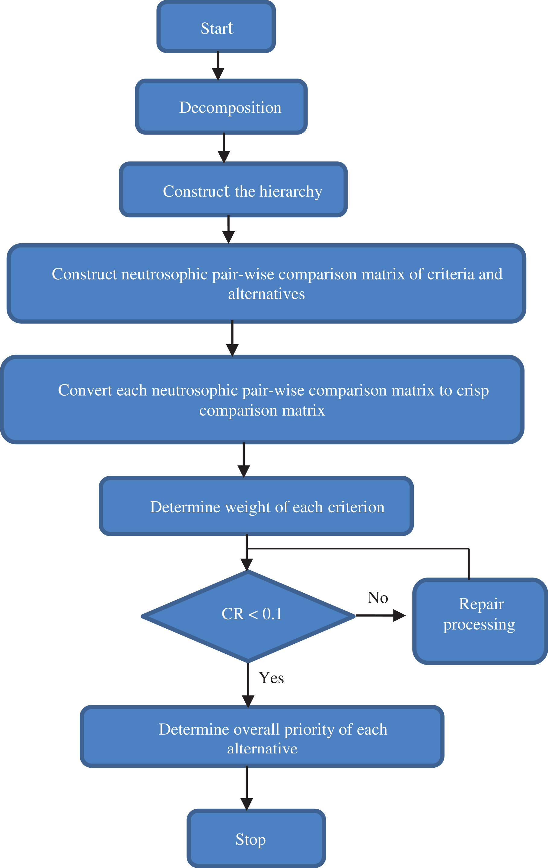
Schematic diagram for solving neutrosophic AHP.
The problem is formed hierarchically at various levels. The first level of hierarch represents the overall goal, the second level represents the decision criteria and sub-criteria and third level is composed of all possible alternatives.
After analyzing the complex multi-criteria decision making problem into three levels, the pair-wise comparisons used to generate neutrosophic judgment matrix. The vagueness of decision makers is represented by triangular neutrosophic numbers
Let
And
Is called the score and accuracy degrees of
To get score and accuracy degree of
With compensation by score value of each triangular neutrosophic number in neutrosophic pair-wise comparison matrix, we have the following deterministic matrix;
From the previous matrix we can easily find ranking of priorities, namely the Eigen Vector X as follows: Normalize the column entries by dividing each entry by the sum of the column. Take the totality row averages.
To calculate CI and CR do the following steps: Multiply each value in the first column of the pair-wise comparison matrix by the priority of the first item; continue this process for all columns of the pair-wise comparison matrix. Sum the values across the rows to get a vector of values labeled “weighted sum” Divide the elements of the weighted sum vector by the corresponding priority for each criterion. Compute the average of the values found in step 2; this average is denoted λ
max
. Compute the consistency index (CI) as follows: Compute the consistency ratio, which is defined as:
This example illustrates the evaluation process of applicants for job. Zagazig University, Egypt announced its need for a database developer to information technology center. An expert in workforce selection of the university has nominated five applicants for this job by conducting a personal interview of applicants. The expert wants to select only one applicant from the five candidates and for this reason the expert based its evaluation process on the following criteria: Presentable Year of experience Age
The previous criteria were considered the most important criteria for selecting the best applicant for the job according to expert opinion. The pair-wise comparison inputs were taken from workforce expert. The methodology illustrated in previous section is used to assign weights and calculate alternatives priorities.
The problem is formed hierarchically at various levels as shown in Fig. 2. The first level of hierarch represents the overall goal (evaluation of job applicants), the second level represents the decision criteria(presentable, years of experience, age) and third level is composed of all possible alternatives (applicant 1, applicant 2, applicant 3, applicant 4, applicant 5).
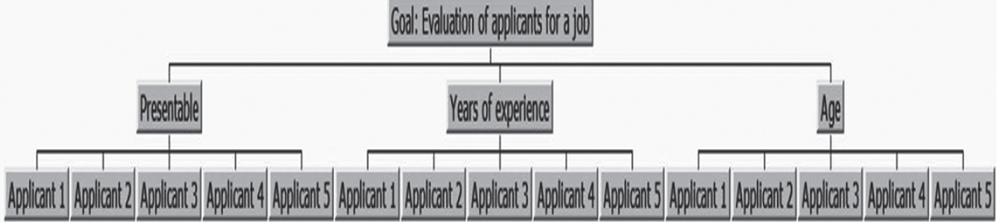
Hierarchy tree of evaluating job applicant’s problem.
The neutrosophic pair-wise comparison matrix of criteria as in Table 4.
Neutrosophic pair-wise comparison matrix of criteria
Where,
By using Equations (4) and (6), the previous neutrosophic pair-wise comparison matrix transformed to deterministic pair-wise comparison matrix as in Table 5.
The deterministic pair-wise comparison matrix of criteria
To calculate the weight of each criterion, we apply the following steps: Normalize the column entries by dividing each entry by the sum of the column. Take the overall row averages.
The previous pair-wise comparison matrix takes the following form:
Column sum = 10/3 7/4 8
Then, the new matrix after normalized column sums is as follows:
Column sum = 1 1 1
From the previous matrix we can easily find ranking of priorities, namely the Eigen Vector X by taking overall row averages as follows:
The ranking of priorities according to the Eigen Vector X are shown in Fig. 3.

Priorities of criteria with respect to goal.
It can be seen from Fig. 3 that years of experience is the most important selection criteria with a weight of 0.500 followed by presentable. Age is the least important criterion.
To ensure that all inputs of expert are consistent we should make a consistency test as follows:
Calculate consistency index and consistency ratio as follows:
From Equations (8) and (9), λ
max
= average{0.97/0.32, 1.69/0.55, 0.37/0.125} = 3.02 and
To calculate the consistency ratio (CR), we used Table 6 which derived from Saaty book. The upper row is the order of the random matrix, and the lower row is the corresponding index of consistency for random judgments.
Saaty table for calculating consistency ratio
Because 0.02<0.1, so the evaluations are consistent.
Neutrosophic pair-wise comparisons of applicants according to presentable criterion are shown in Table 7.
Pair-wise comparison of applicants according to presentable criterion in neutrosophic environment
Where,
By using Equations (4) and (6), the previous neutrosophic pair-wise comparison table transformed to deterministic pair-wise comparison as shown in Table 8.
Pair-wise comparison of applicants according to presentable criterion in deterministic environment
Normalized values for presentable criterion
Normalization of column sums is shown in Table 9.
By taking the overall row average of previous table, then priority vector as follows:
By comparing applicants according to years of experience criterion in neutrosophic environment, the results are shown in Table 10.
Pair-wise comparison of applicants according to years of experience criterion in neutrosophic environment
By using Equations (4) and (6), the previous neutrosophic pair-wise comparison table transformed to deterministic as shown in Table 11.
Pair-wise comparison of applicants according to years of experience criterion in deterministic environment
Normalization of column sum is shown in Table 12.
Normalized values for years of experience criterion
By taking the overall row average of previous table, then priority vector as follows:
By comparing applicants according to age criterion in neutrosophic environment, the results are shown in Table 13.
Pair-wise comparison of applicants according to agecriterion in neutrosophic environment
By using Equations (4) and (6), the previous neutrosophic pair-wise comparison table transformed to deterministic as shown in Table 14.
Pair-wise comparison of applicants according to agecriterion in deterministic environment
Normalization of column sums is shown in Table 15.
Normalized values for age criterion
By taking the overall row average of previous table, then priority vector as follows:
Then the relative scores for each alternative asfollows:
Finally, the AHP ranking of decision alternatives are shown in Fig. 4.
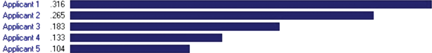
Ranking of alternatives with respect to overall goal.
From Fig. 4 the AHP results indicate that Applicant 1 is the best applicant for job and according to these results, Zagazig University should select Applicant 1 as a database developer of information technology center.
In order to test persistence of the priority ranking, the sensitivity analysis is performed to the AHP results. A weight of 90% is assigned to one criterion and the remaining ratio distributed among the other criteria in the ratio of the oldest weights; this done for all criteria and the final result of AHP is calculated in each case. Different types of sensitivity graphs of AHP results are shown form Figs. 5 to 16.

Dynamic sensitivity analysis.

Dynamic sensitivity analysis by changing priorities.
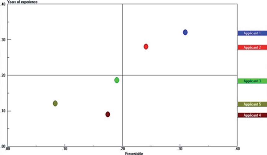
Two dimensional sensitivity analysis of alternatives according to Presentable and Years of experience criteria.
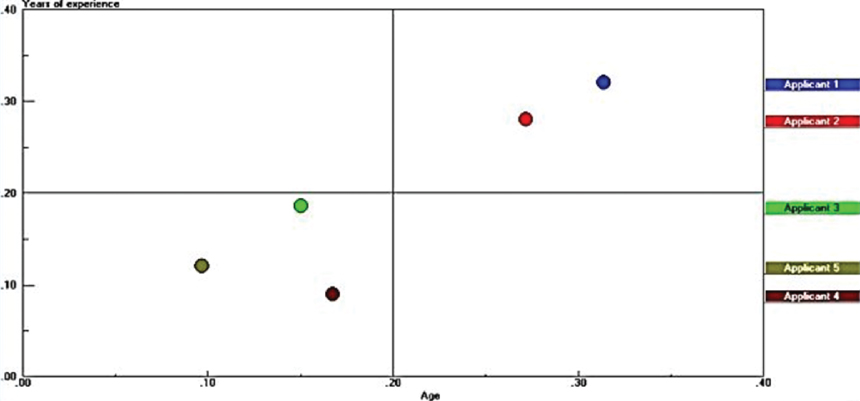
Two dimensional sensitivity analysis of alternatives according to Age and Years of experience criteria.

Head-to-Head sensitivity between Applicant 1 and Applicant 2.
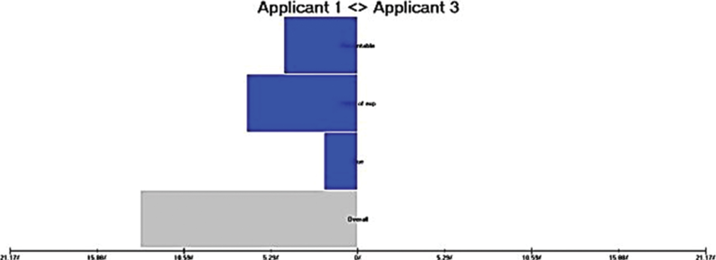
Head-to-Head sensitivity between Applicant 1 and Applicant 3.

Head-to-Head sensitivity between Applicant 1 and Applicant 4.
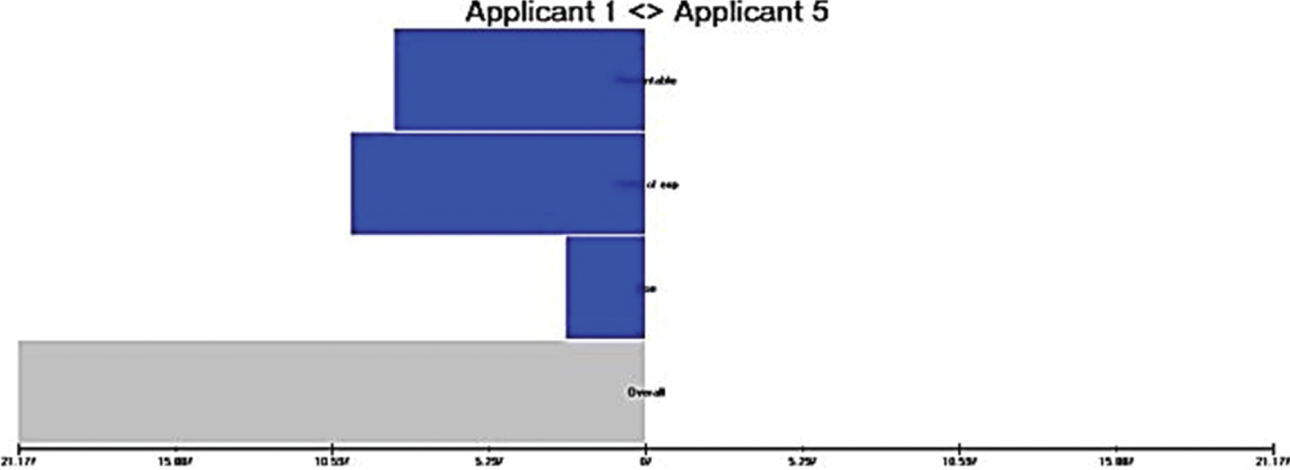
Head-to-Head sensitivity between Applicant 1 and Applicant 5.

Gradient sensitivity for Presentable criterion with respect to overall goal.
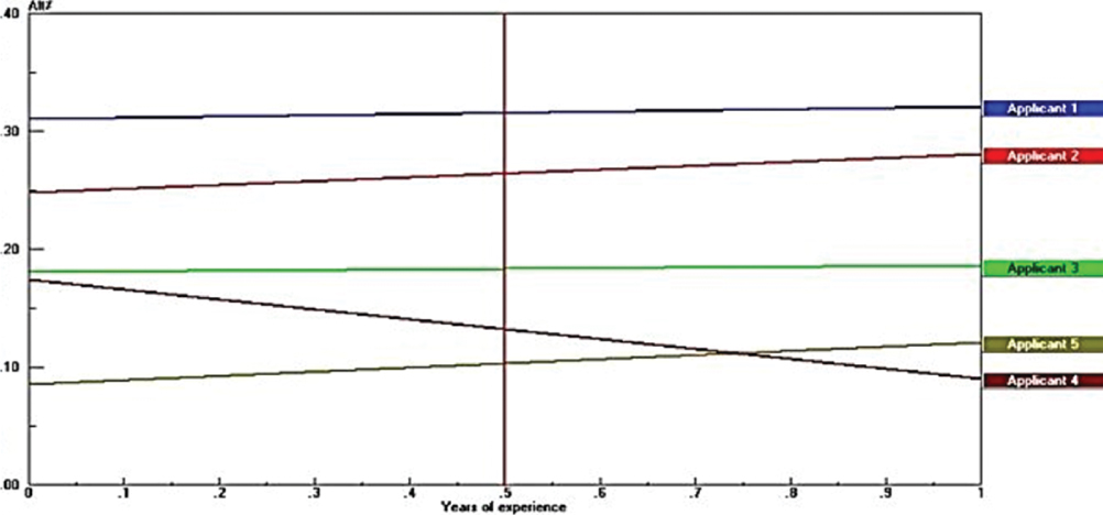
Gradient sensitivity for Years of experience criterion with respect to overall goal.

Gradient sensitivity for Age criterion with respect to overall goal.

Sensitivity analysis graph of the AHP results.
From Fig. 5 the priorities of the alternatives will change in the right column (alternatives column) by dragging the objectives priorities forward and backward in the left column (criteria column).
The decision maker can drag objective’s bar forward or backward to increase or decrease the priority of objectives and see the impact on alternatives as in (Fig. 6).
The second type of sensitivity analysis is the two dimensional sensitivity. The two dimensional sensitivity compare each alternative according to criteria in a two dimensional manner. From Figs. 7 and 8 it’s obvious that the first alternative (Applicant 1) is the best alternative according to years of experience, presentable and Age criteria.
Another type of sensitivity analysis is the Head to Head sensitivity analysis. The Head to Head sensitivity analysis of the AHP results is shown from Figs. 9 to 12. In Head to Head sensitivity each alternative compare with another alternative according to all criteria.
From Figs. 9 to 12 we can conclude that according to Head-to-Head sensitivity of AHP results, Applicant 1 is the best alternative compared to other alternatives.
Figures 13 to 15 illustrates the gradient of each alternative according to each criterion. The previous figures of gradient sensitivity show that Applicant 1 is the best alternative according to allcriteria.
We can gather the previous results of sensitivity in the following graph:
The overall sensitivity graph of the AHP results is shown in Fig. 16. The scores of the alternatives are on the y-axis and the criteria are on the x-axis. From Fig. 16 it’s obvious that Applicant 1 is the best alternative among the five alternatives.
Neutrosophic set includes classical set, fuzzy set and intuitionistic fuzzy set as it doesn’t mean only truth-membership and falsity- membership but also considers indeterminacy function which is very obvious in real life situations. In this research, we have considered parameters of AHP comparison matrices as triangular neutrosophic numbers and we used score function to transform neutrosophic AHP parameters to deterministic values. In the future this research will be extended to trade with different MCDM techniques such as alpha-discounting, nonlinear alpha-discounting and interval alpha-discounting methods.
Footnotes
Acknowledgments
We all want to thank anonymous for the constructive suggestions that improved both the quality and clarity of the research.