Research on spoken English analysis model based on transfer learning and machine learning algorithms

Abstract

From the current situation, it can be seen that there are certain deficiencies in the current models of spoken English analysis. In order to improve the English spoken analysis effect, this study builds an English spoken analysis model based on transfer learning and analyzes the performance of spoken English recognition. In order to make full use of the characteristics of speech feature modes to compensate for the shortcomings of single mode in speech recognition, this paper proposes a multimodal shared speech feature learning method, that is, multimodal shared speech feature learning method based on locality, sparsity, and identifiable typical correlation analysis. The method introduces locality, sparsity and discriminability, and the method effectively improves the English spoken recognition effect to a certain extent. In addition, this paper designs a controlled experiment to analyze the performance of the system model. The research results show that the algorithm has certain effects and can be applied to practice.

Keywords

Transfer learning spoken English speech recognition system model feature analysis

1 Introduction

Speech is the basic means of communication between people and an important way of expressing emotions. Speech emotion recognition, as an important branch of emotional computing, has gradually attracted people’s attention. The earliest research on speech emotion recognition appeared in the mid-1980s, and researchers at that time used the most basic acoustic features to classify emotions [1]. With the development and continuous development of emotional computing, more and more researchers have begun to study speech emotion recognition. Since the 21st century, with the continuous development of speech emotion recognition technology, it has appeared in people’s work, study and life. For example, in the entertainment life, Microsoft Xiao Bing can understand human emotions, and can express emotions such as tone and intonation like human beings, which has become the robot with the strongest chat ability. In the industry, the intelligent in-vehicle system can judge the emotional state of the driver through the form of voice question and answer. If the driver is found to have strong emotional changes, the system can appropriately appease or remind the driver to avoid the occurrence of traffic accidents. In medicine, diseases such as depression require long-term communication between people, and emotional interaction with the machine can effectively solve the problem of lack of medical human resources [2].

The purpose of speech recognition is to identify the emotional state of an audio, so a description of the emotional state needs to be given. Secondly, the premise of speech emotion recognition is to have sufficient data to train the model, so it is necessary to construct a speech emotion database. Moreover, the speech emotion recognition system is mainly composed of two parts: the front end and the back end. The front end is used to extract features, and the back end is designed based on these features [3].

From the initial stage of development, speaker recognition technology is intertwined with practical applications, which can be said to be technological development driven by actual needs. Moreover, the basic way of communication between people and human beings is an inevitable element of human society, which has naturally attracted the interest of many researchers. After every breakthrough in basic technology research, some people will apply this technology to the field of speaker recognition, which will push the speaker recognition technology to a new level. In today’s society, speaker recognition technology has quite a wide range of application requirements [4].

As the most widely used language, English speech intelligent recognition technology has certain practical effects. From the current situation, it can be seen that there are certain deficiencies in the current models of spoken English analysis. In order to improve the English spoken analysis effect, this study builds an English spoken analysis model based on transfer learning based on the transfer learning algorithm, and analyzes the performance of spoken English recognition.

2 Related work

With the rapid development of digital signal processing technology, the field of speech recognition has begun to enter a new development period, because at this time we can directly use the computer for semantic and speaker recognition [5]. Welch [6] applied template matching and statistical analysis of variance to speaker recognition. Bialous [7] applied cepstrum techniques to speaker recognition. Cook. Atal [8] applies linear predictive cepstral coefficients to speaker recognition; Lasheng Y [9] uses formant techniques for speaker recognition in speaker recognition. Ovetz R. Atal [10] then used the fundamental frequency profile for speaker recognition related research. During this period, the development of speaker recognition mainly relies on the extraction of identification parameters.

The research progress of speech recognition is mainly reflected in the linear or nonlinear processing of acoustic parameters and the new pattern matching method. The concept of the Mel Frequency Cepstral Coefficient (MFCC) was proposed by Yang Y F [11] at this time. In terms of models, some important techniques for speaker recognition, such as dynamic time warping, vector quantization [12], and Hidden Markov Model (HMM) [13] have developed dramatically during this period.

With the further development of computer technology, the development of speech recognition has been pushed to a new level. The classical Gaussian mixture model was proposed by Okoh E [14] during this period. GMM is a generation model with simple flexibility and good robustness. It is still the mainstream technology of text-independent voiceprint recognition. In addition, Artificial Neural Network [15] and Support Vector Machine (SVM) [16] have also been applied to the field of voiceprint recognition and achieved good results. Ruolan L [17], the proponent of GMM, further proposed the UBM-MAP (Universal BackgroundModel, Maximuma Posterior) model, which laid an important foundation for speaker recognition from the laboratory to practical. The reason is that the previous GMM training model requires a large amount of voice data, which is difficult to obtain in practical practice, while UBM-MAP can adapt a good model with only a small amount of data based on the existing data. After that, new technologies have sprung up, such as Graph Matching, SVM combined with GMM, high-level speech discussion, multi-modal recognition, and Speaker Model Synthesis (SMS) for channel mismatch problems. Moreover, the research hotspot of speech recognition is transformed into super vector technology. The feature vector set is usually used as a feature of a piece of speech, while the super vector technique uses a fixed-size high-dimensional single vector as a feature of a piece of speech, even if the time length of the speech is different.

In traditional speech recognition, training data and test data generally come from the same corpus or have the same data distribution. With the explosive growth of data, voice data obtained from different devices and environments often differ greatly in terms of language, emotional expression, emotional marking scheme, acoustic signal conditions, and content. This results in a difference in the distribution of training data and test data, and the traditional method of speech emotion recognition is no longer applicable. In recent years, the concept of transfer learning has been proposed, and its main meaning is to transfer useful information from one or more source domains to related target domains, thereby helping to improve the classification performance of the target domain. Domain adaptation, as a special and widely used transfer learning, has been successfully applied to speech recognition across libraries.

3 Automatic encoder

In recent years, neural networks have been applied in many fields, such as image processing, speech processing, and emotion recognition. The next step is to introduce the automatic encoder and several variants.

The ordinary auto-encoder (AE) is mainly composed of two parts of encoding and decoding, as shown in Fig. 1.

Fig.1

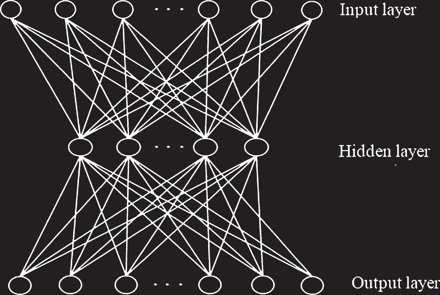
Ordinary automatic encoder.

The coding part maps the input data g into the hidden layer feature h (x) ∈ R^{d
_h}, and the hidden layer feature can be considered as a high-level nonlinear representation of the input data. If the number of hidden layer nodes is less than the number of input layer nodes, then it can be considered that the original input data is compressed. If the number of hidden layer nodes is greater than the number of input layer nodes, it can be considered as an overcomplete representation of the input. The specific formula is as follows:

$h (x) = f (x) = s (Ux + c)$ (1)

In the formula, s (x) = 1/ -(1 + exp(- x)). The function f is a nonlinear activation function, and the commonly used activation functions are sigmoid and tanh functions. U represents the weight matrix of d_h × d_x, and c ∈ R^{d
_h} represents the bias. The decoder maps the feature representation of the hidden layer to the reconstructed $\hat{x}$ of the original input x by minimizing the reconstruction error. The specific formula is as follows:

$\hat{x} = g (h (x)) = s_{g} (U^{'} h (x) + b)$ (2)

In the formula, s_g is the decoding activation function, generally using the sigmoid function. U^′ and b ∈ R^{d
_x} represent the weight matrix and offset of the decoding function, respectively. Generally, it can be set to U′ = U^T, which is called bundle weight. The parameter set for the autoencoder is θ ={ U, b, c }. Then, the minimum reconstruction error function of AE can be expressed as:

$J_{AE} (θ) = \sum_{x \in D} L (x, g (h (x)))$ (3)

In the formula, L is the reconstruction error function. If the decoding activation function s_g is linear, the mean square error can be used as the error function, that is $L (x, \hat{x}) = {∥ x - \hat{x} ∥}^{2}$ . If s_g is a sigmoid function, then the loss function can use cross-entropy, which is: $\begin{matrix} L (x, \hat{x}) = \sum_{k = 1}^{d_{x}} \\ [x_{k} log {\hat{x}}_{k} + (1 - x_{k}) log (1 - {\hat{x}}_{k})] \end{matrix}$

The most common one is the mean square error form. A weight decay is usually added after the AE objective function to prevent over-fitting. Therefore, the objective function of AE can be expressed as:

$\begin{matrix} J_{AE + wd} (θ) = \sum_{x \in D} L (x, g (h (x))) \\ + γ \sum_{ij} U_{ij}^{2} \end{matrix}$ (4)

In the formula, the hyperparameter γ is used to control the proportion of the reconstruction error term and the weight attenuation term. The optimization method of the automatic encoder generally uses a gradient descent method. The update method for weights and offsets is:

$\begin{matrix} U_{ij} : = U_{ij} - α \frac{\partial J_{AE + wd} (θ)}{\partial U_{ij}} \\ b_{i} : = b_{i} - α \frac{\partial J_{AE + wd} (θ)}{\partial b_{i}} \end{matrix}$ (5)

In the formula, α is the learning rate. The automatic encoder has a variety of methods to deform, one method is to add the appropriate penalty items to the original automatic encoder to achieve sparse purpose, forming a sparse automatic encoder (Sparse Auto-Encoder, SAE). We assume that the node value of the j-th hidden layer in the hidden layer is represented by h_j (x), and ${\hat{ρ}}_{j} = \frac{1}{D_{n}} \sum_{i = 1}^{D_{n}} [h_{j} (x^{(i)})]$ represents the average activation degree of the hidden layer node j on the training set. By suppressing the activation of most hidden layer nodes, the purpose of sparseness can be achieved, that is, the average agonistic ${\hat{ρ}}_{j}$ is closer to zero. A positive ρ, which is closer to 0, is selected as the sparse target to make ${\hat{ρ}}_{j}$ closer to ρ, that is ${\hat{ρ}}_{j} \approx ρ$ . To measure the degree of dispersion between ${\hat{ρ}}_{j}$ and ρ, a KL divergence penalty term is introduced, which can be expressed as:

$\begin{matrix} \sum_{j = 1}^{D_{n}} KL (ρ | {\hat{ρ}}_{j}) = \sum_{j = 1}^{D_{n}} \\ ρ log \frac{ρ}{{\hat{ρ}}_{j}} + (1 - ρ) log \frac{1 - ρ}{1 - {\hat{ρ}}_{j}} \end{matrix}$ (6)

After the sparse penalty term is added to the automatic encoder, a sparse autoencoder is formed. Therefore, the objective function of SAE can be expressed as:

$\begin{matrix} J_{SAE} (θ) = J_{AE + wd} (θ) \\ + β \sum_{j = 1}^{D_{n}} KL (ρ ∥ {\hat{ρ}}_{j}) \end{matrix}$ (7)

In the formula, β controls the proportion of the sparse penalty term in the entire objective function.

Another method is to add randomness to the original auto-encoder to form a denoising auto-encoder (DAE). The idea of a denoising autoencoder is simple. It uses the impaired input data to train the autoencoder to reconstruct the corresponding clean input, that is, to force the hidden layer unit to find more robust features. There are many ways to obtain corrupted data. We can manually process a part of the eigenvalue of the input data to 0 or use the noise function to process the input data. If the clean input data and the damaged data are assumed to be x and x_c, respectively, the objective function of DAE can be expressed as:

$J_{DAE} (θ) = \sum_{x \in D} L (x, {\hat{x}}_{c})$ (8)

In the formula, ${\hat{x}}_{c}$ denotes the reconstruction of x_c obtained by the basic automatic encoder.

The third method is the Contractive Auto-Encoder (CAE). In order for the hidden layer to find better features and force h (x) to be robust, we can punish its sensitivity to the input data. This sensitivity can be measured by the F-paradigm of the Jacobian matrix. Therefore, the formula for the penalty function of the contractile activation function can be expressed as follows:

${∥ J (x) ∥}_{F}^{2} = \sum_{i = 1}^{d_{h}} {(h_{i} (1 - h_{i}))}^{2} \sum_{j = 1}^{d_{h}} U_{ij}^{2}$ (9)

Therefore, the objective function of CAE is:

$J_{CAE} (θ) = \sum_{x \in D} L (x, g (h (x))) + λ {∥ J (x) ∥}_{F}^{2}$ (10)

In the formula, λ controls the proportion of the Jacobian penalty term in the entire objective function.

The extraction and expression methods of traditional manual features are highly dependent on human experience, and the adjustment process is very time consuming. Compared with the extraction process of manual features, the automatic feature learning method has the ability to automatically explore and learn features and can learn more representative features of high-level from the underlying features of complex scenes. Therefore, it can improve the ability to predict, identify and classify. Because the changes in facial expressions are very subtle, it is difficult to identify and classify them based on the underlying features such as pixel features. At this time, the deep feature learning method can be used to perform emotion recognition and classification by abstracting the underlying features into a higher-level semantic feature that can directly represent facial expressions, thereby enabling better emotion recognition. For speech signals, emotional recognition of speech is difficult through intuitive perception. Constructing deep automatic feature learning method is an effective method for speech emotion recognition. After extracting the depth visual and speech features, the multi-modal shared features can be formed by the fusion rules, and finally the multi-modal emotion recognition is realized.

Based on the above theory, this paper will try to use the sparse auto-encoder to study the multi-modal emotion recognition of visual speech, and further explore the feasibility and effectiveness of sparse auto-encoder in multi-modal emotion recognition research.

4 Transfer learning

4.1 Traditional transfer learning

When performing feature learning and classification, traditional machine learning must ensure that the data in both the training set and the test set are from the same database, that is, the training data and the test data are subject to the same distribution. However, in many cases, this assumption is not fully satisfied. There are usually many situations, such as training data expiration, that is, data that has already been calibrated is discarded, and a large amount of data is recalibrated. The goal of transfer learning is to use the knowledge learned from an environment to help with learning tasks in the new environment. That is, there is currently only a small amount of new tagged data, but there is a large amount of old tagged data. By picking valid data from the old data, it is added to the current training data to train the new model. The essence of transfer learning is the reuse of knowledge. Next, we introduce the related concepts of transfer learning.

Transfer learning: source domain data D_s and source domain task T_s, target domain data D_T and target domain task T_T are given. Transfer learning is mainly to study how to use the source domain data and source domain tasks to improve the learning task effect of the target domain data. Generally speaking, D_s ≠ T_s, D_T ≠ T_T.

Domain: contains sample feature space X and probability distribution P (X).

Task: contains label space Y and function F (·).

When D_s = T_s and D_T = T_T, that is, the source and target domains are the same and the source and target tasks are the same, the problem becomes a machine learning problem. Figure 2(a) is the learning process of traditional machine learning. Figure 2(b) is the learning process of transfer learning. Comparing Fig. 2(a) and (b), we can see that the traditional machine learning method learns each task separately, and each task is independent of each other and does not affect each other. However, transfer learning is to find the relationship between the source domain and the target domain and the source task and the target task to make use of the knowledge in the source domain and the source task as much as possible to improve the learning task effect of the target domain.

Fig.2

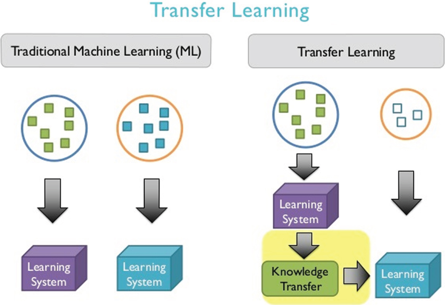
Comparison of the learning process of traditional machine learning and transfer learning.

According to the definition of transfer learning, transfer learning can be divided into three categories: distribution difference transfer learning, feature difference transfer learning, and transition differential transfer learning. Table 1 compares the differences between the three types of transfer learning in the source and target domains. It can be seen from the table that the distribution of the difference between the learning source domain and the target domain data is different or the conditional probability distribution is different, and the feature space of the source and target domain data of the feature difference transfer learning is different, and the data label space of the source domain and the target domain of the transition difference transfer learning is different.

Table 1

Comparison of three types of transfer learning methods

Types	The difference between the source domain and the target domain
Distributed difference transfer learning	Edge distribution or conditional probability distribution is different
Feature difference transfer learning	Feature space is different
Change difference transfer learning	Data tag space is different

In recent years, the research work on transfer learning is mainly divided into three categories: instance-based transfer learning in isomorphic space, feature-based transfer learning in homogeneous space, and transfer learning in heterogeneous space. The basic idea of instance-based transfer learning in isomorphic spaces is to find examples suitable for use as test data from the auxiliary training data and transfer them to the learning of source training data. This transfer learning has a strong knowledge transfer ability. The basic idea of feature-based transfer learning in isomorphic spaces is to use the mutual clustering algorithm to simultaneously cluster the source data and the auxiliary data to obtain a common feature representation. Transfer learning is achieved by representing the source data in this new space. This transfer learning method has a broader knowledge transfer capability. Transfer learning in heterogeneous space is dedicated to solving the problem that source data and test data belong to two different feature spaces and has extensive learning and expansion capabilities.

The three most important issues in traditional transfer learning are: (1) What is the transfer, that is, to find the same part of the knowledge of the source domain and the target domain or the source task and the target task. (2) How to transfer, that is, to find the right way to transfer the same part of the knowledge. (3) When to transfer, that is, to explore the conditions for knowledge transfer. That is to say, knowledge transfer under this condition is beneficial to improve the performance of the target, and also to explore the conditions for the inability to carry out knowledge transfer.

4.2 Multimodal transfer learning

The source and target domains of traditional transfer learning are homogeneous data from the same database, that is, data with the same distribution, such as the source domain and the target domain are from the expression database or the voice emotion database. However, most of the data in real life comes from different databases and have different distributions, and even there is a phenomenon of data loss, so the traditional transfer learning method is not suitable for this case. The multimodal transfer learning method is to learn the knowledge transfer between modals with different types and distributions of modal data, and this method can also be used to solve the problem of modal missing. The first condition for knowledge transfer between different types of data (modal) is that a shared projection space can be learned in which different modal information can be shared. Then, the common projection methods are mainly the following:

The first is multivariate support vector regression: This method expresses the mapping between two conceptual spaces as a multivariate regression problem. Specifically, under the premise that the source space is given, the support vector regression method with nonlinear kernel can effectively learn the conditional expectation of the target space.

The second is KNN-based Non-parametric mapping: This method finds the K closest source domain samples in the training set and obtains the corresponding target domain samples. The average of the corresponding target domain samples is then used as a mapping for the source domain. After the training data pairs of M video and speech are given, the similarity between the video sample x and the speech sample y can be expressed as: $\begin{matrix} σ (x, y) = cos (x, x^{'}) x^{'} = = \arg \max_{y^{'} \in T} cos (y, y^{'}) \end{matrix}$

That is, the average value y′ of the k-number of speech data closest to the speech sample y is first found from the training set and the similarity between x and m associated with y′ is calculated. It can be seen that σ (x, y) and σ (y, x) are different because the former is considered from the perspective of video space, and the latter is considered from the perspective of speech space.

The third is the normalized canonical correlation analysis (NCCA): taking visual and speech modalities as an example, it assumes that there are N pairs of video and speech data, and H_A ∈ R^N×p and H_V ∈ R^N×p represent the high-level features of speech and video, respectively. The NCCA projects the speech and visual signals into a shared space by H_AU and H_VU, and obtains a projection matrix of U ∈ R^p×c and V ∈ R^Q×c.

In the shared projection space, multiple modal information can realize the transfer learning of different modal information and the reconstruction and prediction of missing modal information through the learning of knowledge transfer function or the learning of transfer network.

5 Learning method of visual voice multimodal sharing emotional features

Figure 3 shows the complete model framework. The frame diagram is divided into three phases from left to right, namely: 1) Single-modal high-level emotional feature learning: The sparse auto-encoder (SAE) is used to learn high-level emotional features of visual and speech samples in an unsupervised manner. 2) Multimodal shared emotional feature learning: At this stage, visual and speech shared emotional features are obtained in two steps. First, the shared emotion feature learning method En-SLDCCA is used to obtain the correlation coefficient between modals by maximizing intra-class correlation and minimizing interclass correlation. Next, the obtained correlation coefficient is used as the weight of visual and speech high-level emotional features to form multi-modal shared emotional features. 3) SVM training: The multimodal shared sentiment feature obtained in the previous stage is used as input to train the SVM classifier.

Fig.3

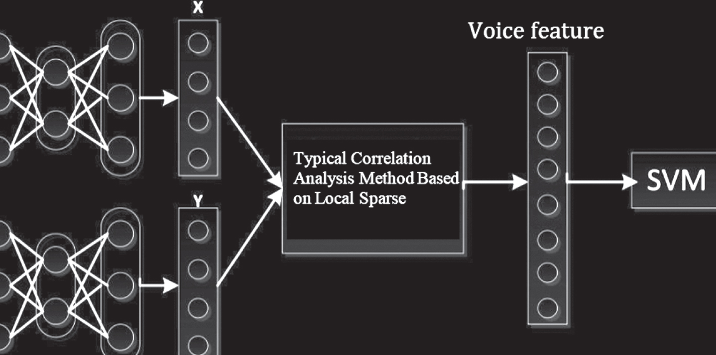
Model frame diagram.

5.1 Single mode high-level emotional feature learning

As shown in Fig. 3(a), the sparse auto-encoder is used to learn the high-level emotional features of the visual and speech samples, respectively. The sparse auto-encoder has two parts: encoding and decoding. The encoding process is to learn a function h through the formula h (x) = f (Wx + b). In the formula, f (z) = 1/ -(1 + exp(- z)) is a nonlinear activation function, W is the weight matrix, and b is the offset vector. The decoding process refers to reconstructing the input samples by minimizing the reconstruction error. The backpropagation algorithm (BP) is used to minimize the reconstruction error $\sum_{i = 1}^{p} {∥ x - \hat{x} ∥}^{2}$ . In order to limit the activation of hidden layer nodes is sparse, we added a rule item.

$J (W, b) = \sum_{i = 1}^{p} {∥ x_{i} - {\hat{x}}_{i} ∥}^{2} + β \sum_{j = 1}^{m} SP (ρ ∥ {\hat{ρ}}_{j})$ (11)

In the formula, $SP (ρ ∥ {\hat{ρ}}_{j}) = ρ log \frac{ρ}{{\hat{ρ}}_{j}} + (1 - ρ)$ $log \frac{1 - ρ}{1 - {\hat{ρ}}_{j}}$ and ${\hat{ρ}}_{j} = \frac{1}{p} \sum_{i = 1}^{p} h_{j} (x_{i})$ . p represents the size of the sparse level, and β controls the weight of the sparse penalty term. If the number of hidden layer nodes is less than the number of input layer nodes, the network can learn a compressed sparse feature of the input layer.

5.2 Multimodal sharing emotional feature learning

We assume that there are N training sample pairs, and X = [x₁, x₂, …, x_N] and Y = [y₁, y₂, …, y_N] represent the high-level features of vision and speech, respectively. The first stage of learning the shared sentiment feature is to obtain the correlation coefficients W_x and W_y by maximizing the correlation between the two modal classes and minimizing the inter-class correlation. The objective function is expressed as follows:

$max_{W_{x}, W_{y}} \frac{W_{x}^{T} S_{xy} W_{y}}{\sqrt{W_{x}^{T} {\hat{D}}_{xx} W_{x} \times W_{y}^{T} {\hat{D}}_{yy} W_{y}}}$ (12)

In the formula, ${\hat{D}}_{xx}$ and ${\hat{D}}_{yy}$ represent the covariance matrix of the visual and speech modes, respectively, which can be expressed as follows:

${\hat{D}}_{xx} = ρ α I + (1 - ρ) S_{xx} {\hat{D}}_{yy} = ρ α I + (1 - ρ) S_{yy}$ (13)S_xx and S_yy in Equation (13) are expressed as follows:

$S_{xx} = X (I - R) {(I - R)}^{T} X^{T} S_{yy} = Y (I - S) {(I - S)}^{T} Y^{T}$ (14)

In the formula, R = [r₁, r₂, …, r_N] and S = [s₁, s₂, …, s_N] respectively represent sparse reconstruction matrices of visual and speech high-level features, which can be calculated by sparsely maintaining the typical correlation analysis method SPCCA. The parameter ρ in Equation (13) can be obtained by using the oracle contraction algorithm:

$ρ = min \frac{(1 - \frac{2}{p}) tr (S^{2}) + t r^{2} (S)}{(N + 1 - \frac{2}{p}) [tr (S^{2}) - \frac{t r^{2} (S)}{P}]}$ (16)

In the formula, α = tr (S)/ -P, P is the matrix dimension.

S_xy in Equation (12) is mainly used to maximize the association within the local class and to minimize the association between the local classes, which can be expressed as follows:

$S_{xy} = S_{w} - μ S_{b}$ (17)

In the formula, S_w represents a local intraclass matrix, and S_b represents a local interclass matrix. S_w and S_b can be expressed as follows:

$\begin{array}{l} S_{w} = \sum_{i = 1}^{N} \sum_{x_{k} \in N^{l} (x_{i}) \cup y_{k} \in N^{l} (y_{i})} x_{i} y_{k}^{T} + x_{k} y_{k}^{T} \\ S_{b} = \sum_{i = 1}^{N} \sum_{x_{k} \in N^{E} (x_{i}) \cup y_{k} \in N^{E} (y_{i})} x_{i} y_{k}^{T} + x_{k} y_{i}^{T} \end{array}$ (18)

Equation (12) is difficult to calculate directly, so it can be converted into the following formula:

${\begin{matrix} (XA Y^{T}) {\hat{D}}_{yy}^{- 1} {(XA Y^{T})}^{T} W_{x} = λ^{2} {\hat{D}}_{xx} W_{x} \\ (XA Y^{T}) {\hat{D}}_{xx}^{- 1} {(XA Y^{T})}^{T} W_{y} = λ^{2} {\hat{D}}_{yy} W_{y} \end{matrix}$ (19)

In the formula, $A = (F_{x} + F_{y}^{T}) - (G_{x} + G_{y}^{T})$ , F_x, F_y, G_x, G_y is expressed as follows: $\begin{matrix} F_{ij}^{x} = {\begin{matrix} 1, if x_{i} \in N^{l} (x_{j}) or if x_{j} \in N^{l} (x_{i}) and L (x_{i}) = L (x_{j}) \\ 0, else \end{matrix} \\ F_{ij}^{y} = {\begin{matrix} 1, if y_{i} \in N^{l} (y_{j}) or if y_{j} \in N^{l} (y_{i}) and L (y_{i}) = L (y_{j}) \\ 0, else \end{matrix} \end{matrix}$ $\begin{matrix} G_{ij}^{x} = {\begin{matrix} 1, if x_{i} \in N^{E} (x_{j}) or if x_{j} \in N^{E} (x_{i}) and L (x_{i}) \neq L (x_{j}) \\ 0, else \end{matrix} \\ G_{ij}^{y} = {\begin{matrix} 1, if y_{i} \in N^{E} (y_{j}) or if y_{j} \in N^{E} (y_{i}) and L (y_{i}) \neq L (y_{j}) \\ 0, else \end{matrix} \end{matrix}$ (20)

Equation (19) can also be solved to obtain the following formula:

$\begin{matrix} (\begin{matrix} {XAY}^{T} \\ {({XAY}^{T})}^{T} \end{matrix}) (\begin{matrix} W_{x} \\ W_{y} \end{matrix}) \\ = λ (\begin{matrix} {\hat{D}}_{xx} \\ {\hat{D}}_{yy} \end{matrix}) (\begin{matrix} W_{x} \\ W_{y} \end{matrix}) \end{matrix}$ (21)

The correlation coefficients W_x and W_y can be obtained by solving the eigenvector matrix corresponding to the eigenvalues in Equation (21).

$Z = W_{x} \times X + W_{y} \times Y$ (22)

With the continuous development and improvement of artificial intelligence technology, speech recognition has gradually become an important research direction in the field of artificial intelligence and human-computer interaction. Moreover, speech recognition, as an important branch of intelligent computing, has attracted the attention of the computer vision field and the speech computing research community. Since single modal information has certain defects in speech recognition, research on multimodal speech recognition has become more and more important. This paper focuses on the study of speech modal information. The general process of multimodal emotion recognition includes three processes: single mode speech feature extraction, multimodal shared feature learning and speech recognition. The fusion method mainly includes feature layer fusion and decision layer fusion. Figures 4 and 5 are the general process of feature layer fusion and decision layer fusion.

Fig.4

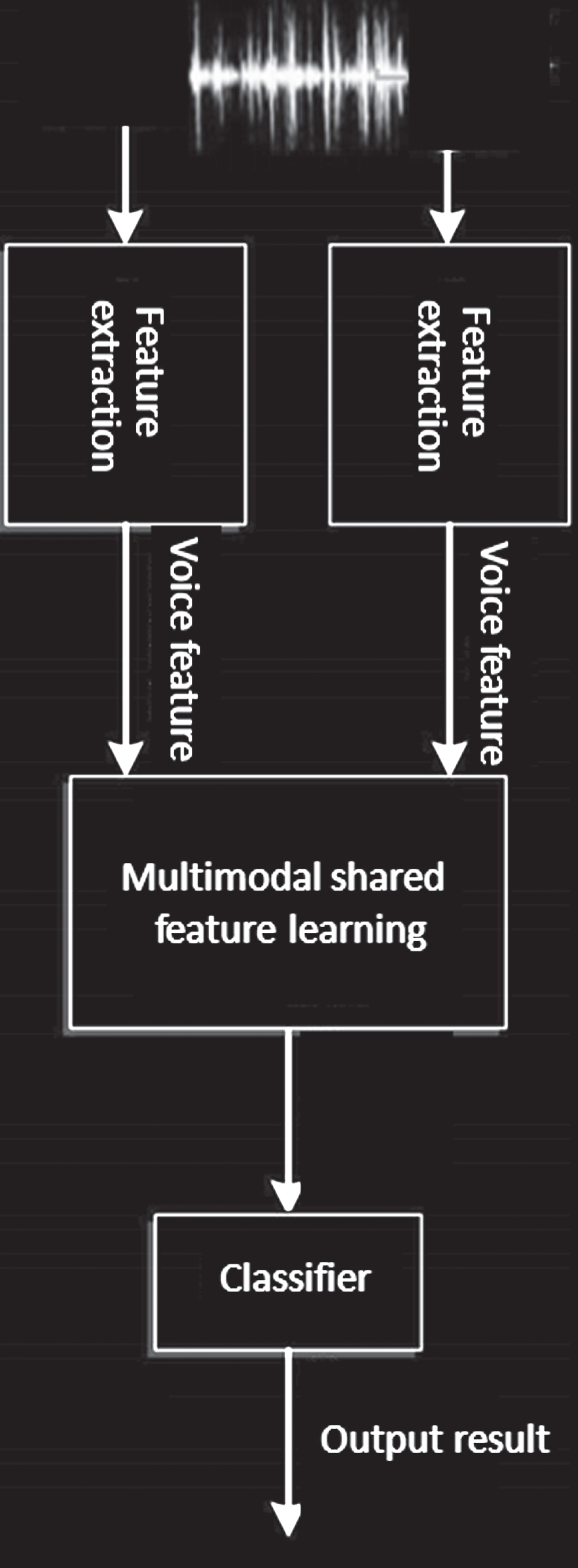
Fusion process of multimodal feature layer.

Fig.5

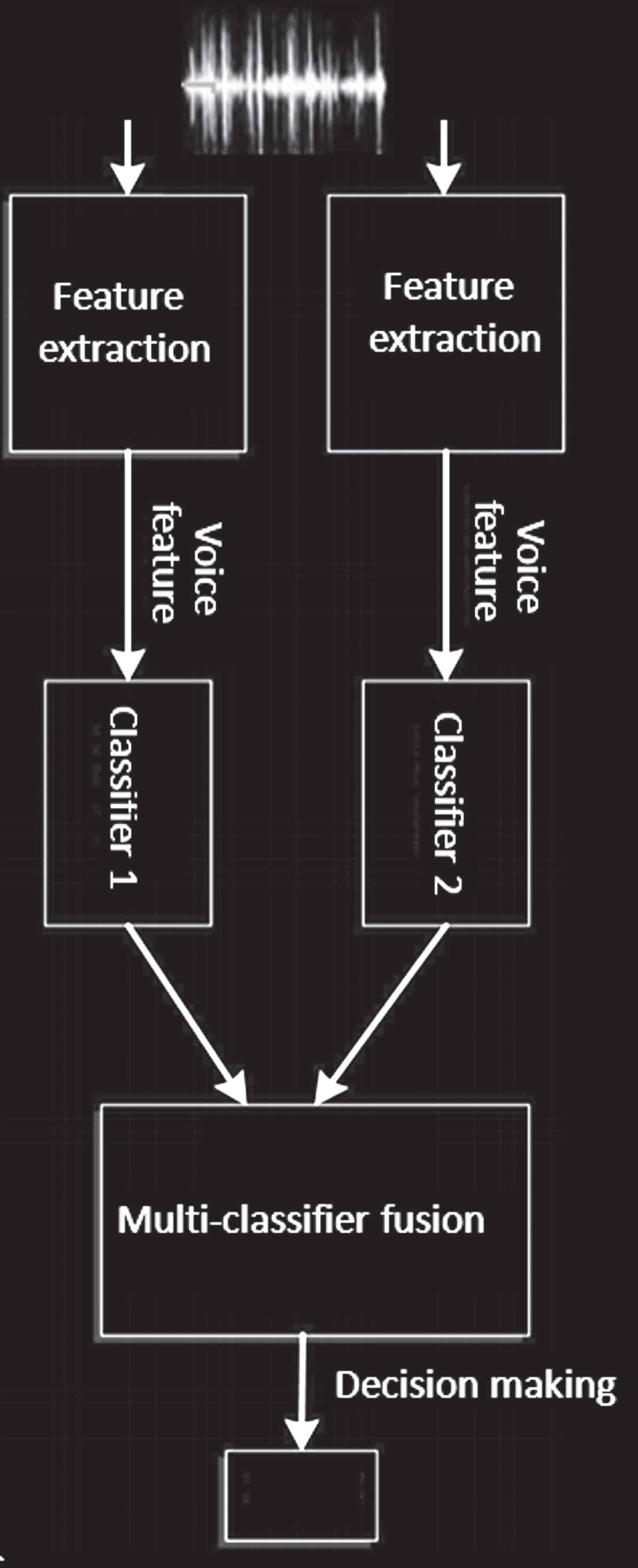
Fusion process of multimodal decision layer.

6 Model building

The premise of the traditional speech emotion recognition method is that the training sample and the test sample are from the same speech library, that is, the data distribution of the two domains is the same. But in reality, this condition is difficult to meet. The reason is that there is a big difference in the voice data collected from different devices and conditions, which make the training data and the test data have different data distributions. Therefore, if we still use the traditional speech emotion recognition model for training and testing (that is, training the model only with source domain data and then directly testing with the target domain), there will be a large performance degradation.

In the case of unsupervised domain adaptation, in the training phase, the algorithm can not only use the tagged data of the source domain, but also use the tagless training data of the target domain. Moreover, how to use the data of these two domains to help improve the classification performance of the target domain is the research focus of the current unsupervised domain adaptation method. At present, some domain adaptation methods can effectively utilize the tagged data of the source domain and the tagless data of the target domain to help improve the classification performance of the target domain. However, in the feature learning process, most domain adaptation methods do not take into account the role of tag information. At the same time, in the domain adaptation method for speech emotion recognition, some advantages of traditional speech emotion recognition (such as considering the speaker, content, environment and other emotion-independent factors in the process of extracting features) are also ignored.

This study considers the role of tag information in the domain adaptation method and proposes a speech feature learning model. Moreover, this study further combines some advantages of traditional speech recognition to propose an improved speech discriminant and domain-invariant feature learning model, the structure of which is shown in Fig. 6.

Fig.6

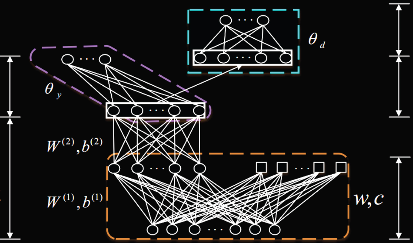
Improved sentiment discrimination and domain invariant feature learning model.

7 Performance study of algorithm model

In order to clearly show the experimental results in this part, the results will be introduced from two parts, namely the ESR system based on feature fusion and model fusion and the confidence measure of ESR system based on model fusion. First, the performance of ESR system based on feature fusion and model fusion is given. In addition to the SVM-based ESR system and the deep learning-based ESR system as the comparison system, in this paper, the input data of the DBN based on the model fusion and the input data of the DBN based on the feature fusion are respectively input into the SVM as a comparison system of the fusion method.

In this paper, when the deep speech features are extracted by the stacked depth auto-encoder network model in deep learning, the MFCC feature is used as the input data of the network node of the model, as shown in Fig. 7. The figure is partial feature data, that is, wherein the number of voice frames of the word is 168 frames.

Fig.7

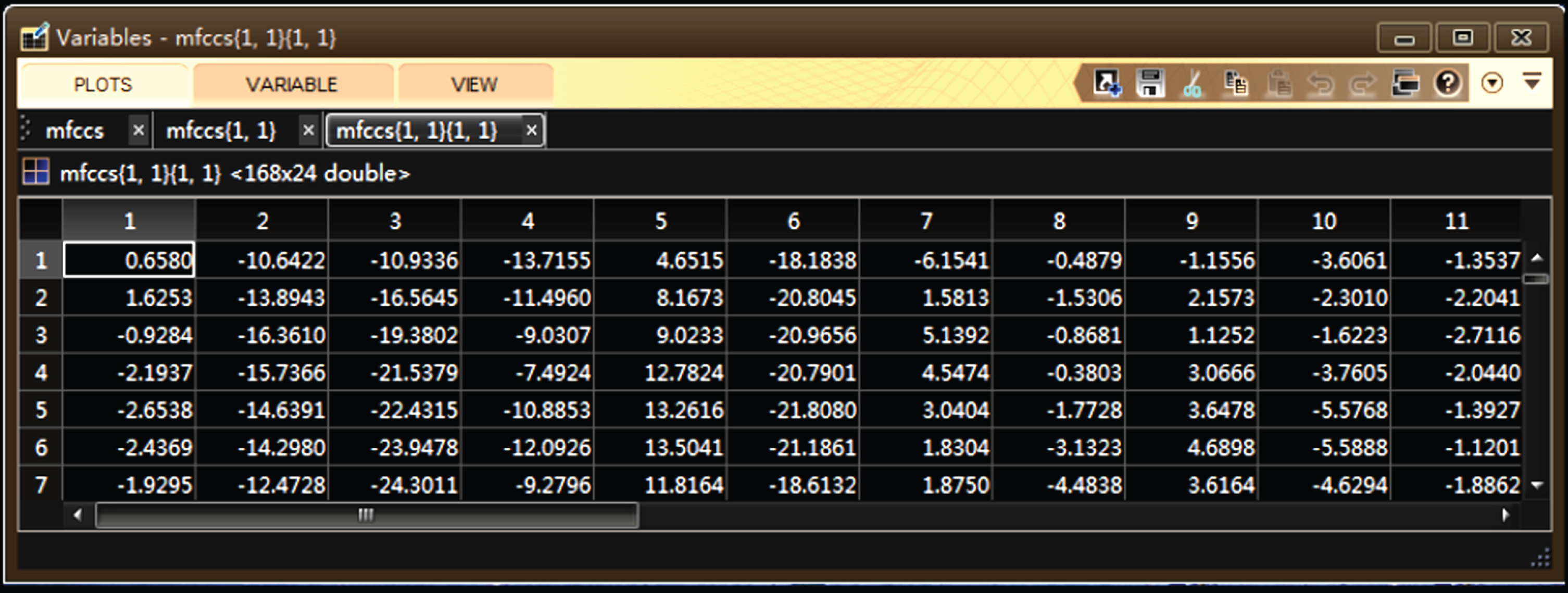
Partial data of the MFCC feature.

The DAE (including the structure of two different training methods: unsupervised and supervised) structure is constructed to extract new acoustic features and train the acoustic model library. The following is an acoustic pattern library that trains 48-dimensional speech features extracted from the 24D MFCC features of the original speech through the unsupervised training of the DAE, as shown in Fig. 8.

Fig.8

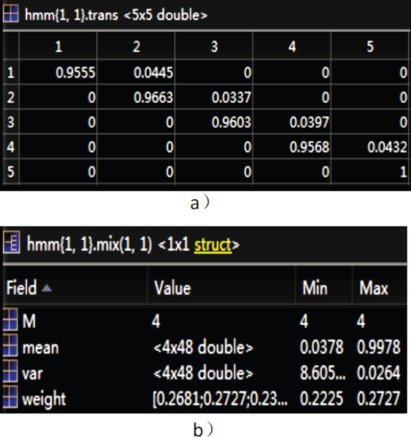
Various parameters after deep feature training.

In the WIFI network condition, the speech recognition effects of each scene in Appendix 2 are tested in turn, and each instruction in each scene is tested 5 times (5 people, 3 men and 2 women, spoken English, office environment). After that, the speech instruction recognition rate is counted, and the test results are shown in Table 2.

Table 2

Statistical recognition results according to the scene

Scenes	Chat mode	Automatic mode	Manual mode	Training mode
Number of instructions	21	17	26	36
Testing frequency	105	75	130	180
Correct number of times	96	70	121	166
Recognition rate	91.40%	93.30%	93.10%	92.20%

It can be seen from Table 2 that the recognition rate of each scene is higher than that of the simple traditional model system. It can be seen from the test results that with the continuous use of the hybrid speech recognition system, the recognition accuracy is higher than that of the traditional speech recognition, and the dynamic multi-scene switching function is realized.

8 Conclusion

As an important aspect of speech computing, spoken English recognition has attracted the attention of many researchers. In the traditional speech recognition, an important research direction is to separate the emotion-related factors and the irrelevant factors of spoken English recognition in the process of English spoken feature extraction, so that the extracted speech features have strong generalization.

This paper studies the influence of transfer learning on English spoken speech recognition system and aims to improve the correctness of word recognition in isolated speech recognition system by using English speech features extracted by transfer learning model.

In order to verify the influence of the deep learning model on the isolated speech recognition system, this paper uses the depth auto-encoder to perform unsupervised and supervised two different deep feature extractions on the original speech features. Moreover, this study retrained the HMM acoustic model using these two different deep features, respectively. The recognition result indicates that the feature extracted by the multi-layer network structure improves the recognition rate. Moreover, the experiment also proves that the new features extracted by the automatic encoder with supervised training using the binary coding marks of the 360 training speeches as the supervised information are more closely related to the recognition task, and its robustness is further enhanced.

References

Rajab

K.D.

, The effectiveness and potential of e-learning in war zones: an empirical comparison of face-to-face and online education in Saudi Arabia, IEEE Access (99) (2018), 1–1.

Baldwin

, Trespalacios

J.H.

, Evaluation instruments and good practices in online education, Online Learning21(2) (2017), 45–50.

Krause

, Hall

, Williams

J.J.

, et al. Connecting online work and online education at scale, Social Science Electronic Publishing26(4) (2017), 3536–3541.

Wolf

R.C.

, Romer

A.K.

, Nord

, New Science, New Media: An Assessment of the Online Education and Public Outreach Initiatives of The Dark Energy Survey, 4(8) (2018), 11–12.

Funes

, Mackness

, When inclusion excludes: a counter narrative of open online education, Learning, Media and Technology (2018), 1–20.

Welch,

Susan.

Virtual mentoring program within an online doctoral nursing education program: a phenomenological study, International Journal of Nursing Education Scholarship14(1) (2017), 22–25.

Bialous

S.A.

, Sarna

, Wells

M.J.

, et al. Impact of online education on nurses’ delivery of smoking cessation interventions with implications for evidence-based practice, Worldviews on Evidence-Based Nursing5(7) (2017), 22–25.

Cook,

Puritz J.

Online education and the emotional experience of the teacher, New Directions for Teaching and Learning2018(153) (2018), 67–75.

Lasheng

Y.U.

, Xu

W.U.

, Yu

, An online education data classification model based on Tr_MAdaBoost algorithm, Chinese Journal of Electronics28(01) (2019), 25–32.

10.

Ovetz

, Click to save and return to course: online education, adjunctification, and the disciplining of academic labour, Work Organisation Labour & Globalisation11(1) (2017), 48–70.

11.

Yang

Y.F.

, Tsai

C.C.

, Exploring in-service preschool teachers’ conceptions of and approaches to online education, Australasian Journal of Educational Technology33(1) (2017), 134–147.

12.

Kolluru

, Varughese

J.T.

, Structured academic discussions through an online education-specific platform to improve Pharm.D. students learning outcomes, Currents in Pharmacy Teaching and Learning9(2) (2017), 230–236.

13.

Amant S,

Kirk.

Of friction points and infrastructures: rethinking the dynamics of offering online education in technical communication in global contexts, Technical Communication Quarterly (2017), 1–19.

14.

Okoh

, Makame

M.H.

, Awad

A.I.

, Toward online education for fingerprint recognition: A proof-of-concept web platform, Information Security Journal: A Global Perspective (2017), 1–12.

15.

Steele

J.R.

, Jones

A.K.

, Clarke

R.K.

, et al. Use of an online education platform to enhance patients’ knowledge about radiation in diagnostic imaging, Journal of the American College of Radiology14(3) (2017), 386–392.

16.

Tse

M.M.Y.

, Tang

, Budnick

, et al. Pain and pain management among university students: online survey and web-based education, Cyberpsychology, Behavior, and Social Networking20(5) (2017), 305–313.

17.

Ruolan

, The Preliminary Exploration of the Application of MOOC in College Oral English Teaching, 8th International Conference on Information Technology in Medicine and Education (ITME), IEEE (2016), 54–60.