
Abstract
Feature extraction is the basis of texture analysis. How to obtain texture features with small feature dimension, simple calculation and comprehensive representation of images is a hot spot and a difficult point in feature extraction. The traditional image texture feature extraction method is to process the image in the spatial domain. However, due to its high computational complexity, its practical application is restricted. Based on this, this study studies the extraction method of texture features, and deeply analyzes the principle of non-subsampled Contourlet transform. Moreover, this study uses NSCT to transform the image from the spatial domain to the frequency domain and extracts the texture features of the decomposed low frequency sub-band, intermediate frequency sub-band and high frequency sub-band image respectively. In addition, this study selects the appropriate parameters to establish the support vector machine model and applies the extracted texture features into the support vector machine for recognition and applies it to the sports feature recognition. Finally, this study designed a controlled experiment to analyze the performance of the algorithm. The results show that the proposed method has certain effects.
Introduction
The method of transforming a texture image into a frequency domain using a linear transformation, filter or filter bank and then extracting texture features in the frequency domain can capture most of the information in the texture image, so it has been widely used [1].
Computer vision measurement technology, as a measurement method that imitates human vision and combines photography technology with computer technology, has shown its importance and broad development prospects [2]. In particular, the three-dimensional motion detection technology based on computer vision can complete accurate, online and non-contact motion detection of large space and multi-target. Its advantage is [3, 17].
Vision is the most important way for humans to feel the objective world. According to statistics, more than 80% of the information in the outside world perceived by human beings is obtained by the visual system [4]. Humans perceive the world through vision, and then through the human brain to understand and transform the world. Computer vision is the imitation of human visual function. It captures the image through the camera at the front end, extracts relevant information from the image or image sequence, and recognizes the shape and motion of the three-dimensional scene and target in the objective world. Computer vision is an information processing process that understands scenes from acquired images. The task of the computer is to use computer technology and related corresponding algorithms to complete the information processing work, so that the computer can establish a concrete and meaningful description of the objective scene based on the visual information, thereby understanding the environment and obtaining useful information. To make computer vision replace human eyes and brain, to complete accurate perception and interpretation of the real world is the goal that science and technology workers are constantly pursuing. The stereo vision-based detection technique refers to a method of acquiring and accurately determining the shape, position and motion of a target to be measured in a three-dimensional space by acquiring image information of a research object [5, 18].
It is widely used due to its non-contact, fast measurement speed, convenient and flexible measurement methods and relatively high measurement accuracy. The stereo vision motion detection system can be generally divided into the following modules: image acquisition module, feature extraction, recognition module, stereo matching module, camera parameter calibration module, spatial point positioning module, and motion parameter calculation module [6, 19]. This research focuses on the intelligent sports recognition system based on support vector machine and promotes the application of computer vision technology in the development of sports industry based on computer vision technology.
Related work
At present, motion detection technology based on computer vision sequence images is mainly applied to virtual reality, robot motion, industrial target motion control, vehicle monitoring, flight target tracking, human motion recognition, biological tissue motion analysis, facial expression recognition [7–9]. In the following, the research status of this subject needs to be analyzed from the classification of motion detection technology based on computer vision sequence images.
Motion detection techniques and systems based on computer vision sequence images have many classification methods. According to the measurement principle of sequence image motion detection technology and related algorithms that have been studied successfully and under study at home and abroad, it can be roughly divided into the following two categories: continuous measurement method based on optical flow and discrete measurement method based on features. The former is mainly suitable for the measurement of short time and small amount of motion. Its basic concept was first proposed by Kuss A [10] in 1950, and it plays an important role in the understanding of moving images. The so-called optical flow refers to the instantaneous velocity field of the movement of pixel points on the observed surface of a moving object in three-dimensional space.
Through the study of the advanced vision system similar to the human eye, it can be shown that the human eye can establish the motion sensation by matching the obvious corresponding features in space under unstable illumination conditions at considerable time intervals, that is, the visual motion target can be tracked in long distance space [11]. Thus, similarly, motion can be detected using methods for tracking and analyzing specific markers in a sequence of images. The feature-based discrete measurement method is based on this principle. It is suitable for measuring the motion parameters of moving targets that are used for long periods of time and large amounts of motion. Moreover, the algorithm implementation is relatively simple, there are some effective linear algorithms, and the requirements for the measurement environment are relatively low, which is more suitable for field production in industrial production and national life [12]. At present, from the practical application, the research on computer vision motion measurement methods based on discrete features has become one of the most challenging and practical topics in the field of computer vision motion detection.
Texture image recognition based on support vector machine
With the generation of large-scale digital images, automatic image classification is a key task in many applications. Texture classification is to assign the texture pattern of an image to a known texture category according to the decision plan of the classifier. At present, texture recognition and classification have been widely applied to various fields such as agriculture, remote sensing, industry, medicine, marine science, and materials science. The basic content of texture classification is to input the extracted texture features into the established classifier model for classification [13]. How to improve the recognition accuracy is a hot and difficult point in texture classification. At present, the commonly used classifiers at home and abroad mainly include K-nearest neighbor method, support vector machine (SVM), neural network, and Bayesian estimation [14].
Statistical Learning Theory (SLT) was produced in the 1960 s and matured in the 1990 s. It is based on machine learning problems under limited sample conditions, which can better solve internship learning problems. In the 1960 s and 1970 s, the theoretical foundations of statistical learning were gradually established. In 1968, V. Vapnik and Chervonenkis proposed [15] the core concept of statistical learning theory, VC dimension theory. In 1982, V. Vapnik further proposed the principle of structural risk minimization, which laid a solid theoretical foundation for the research and establishment of SVM. From 1992 to 1995, Vapnik and his collaborators Boser, Guyon, Cortes and Scholkopf developed the theory of support vector machine (SVM) based on statistical learning theory. Compared with the traditional classification algorithm, the support vector machine can effectively prevent the over-learning phenomenon, solve the local extremum problem that cannot be avoided in the neural network method, and can effectively avoid the dimensionality disaster, and the complexity of the algorithm is independent of the sample dimension. In recent years, there have been many development and improvement of SVM algorithms, such as Zhang Xuegong’s CSVM, Scholkopf’s v-SVM, Joachims’ SVM light and Hsu’s BSVM. These algorithms are improvements to the support vector machine algorithm. The structure of the SVM model was learned through literature search, as shown in Fig. 1. In SVM, the complexity of the construction is independent of the feature space dimension and depends only on the number of support vector machines [16].

Structure diagram of the support vector machine.
When using SVM for classification and recognition, the eigenvectors of the training sample image and the test sample image are extracted separately, and the training sample feature vector is input into the SVM for training to obtain an SVM recognition model. At this time, the test sample feature necklace is input into the obtained SVM recognition model to obtain a test result output. The classification algorithm flow chart is shown in Fig. 2.

Flow chart of the SVM model classification algorithm.
SVM research begins with the analysis of the optimal classification plane in the case of linear separability.
The given training set is:
In the formula, x is the input vector, i is the number of samples, d is the dimension of the input vector, and y is the category to which the input vector belongs.
The hyperplane equation in the case of linear separability is:
In the formula, w is the normal vector of the hyperplane, and b is the distance of the hyperplane from the origin.
The optimal classification line requires that the classification line not only correctly separate the two types, but also maximize the classification interval, as shown in Fig. 3. After being promoted to a high-dimensional space, the classification line is the classification surface. In the figure, solid points and hollow points represent two types of samples, and H is the optimal classification line. H1 and H2 are the straight lines of all kinds of samples that are closest to the classification line and parallel to the classification line. The distance d between them is called the classification interval (margin).
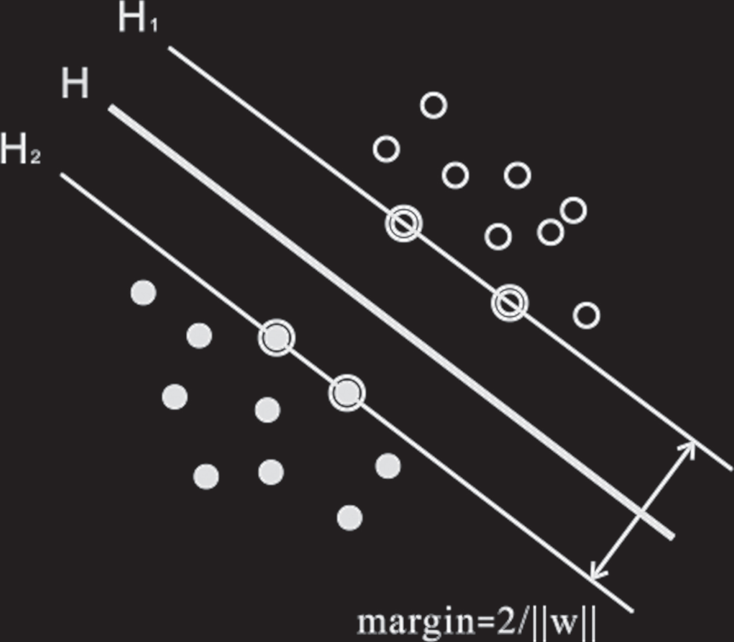
Schematic diagram of the optimal classification surface.
From Equation (3), it can be obtained that the classification interval is 2/ -∥ w ∥. Therefore, the maximum classification interval is equivalent to minimizing ∥w∥. Therefore, the classification surface that satisfies the Equation (3) and has the largest classification interval is called the optimal classification surface. The training sample points on H1 and H2 are called support vector machines. Maximizing the classification interval refers to the control of the promotion ability, which is one of the core ideas of the support vector machine.
For the linear separable case, it is necessary to minimize the functional solution to solve the optimal hyperplane under constraint (2).
This optimization problem can be solved by introducing a Lagrangian function:
In the formula, α
i
is a Lagrangian multiplier. Through the optimal solution condition (Karush-Kuhn-Tuchke condition), the above optimization problem can be transformed into the dual problem of Equation (2). The maximum functional is:
The constraints are:
This is a quadratic programming problem with inequality constraints, so there is a unique solution. Only the support vector SV can have a non-zero coefficient α
i
. The final decision function is:
For the linear indivisible case, in order to construct the optimal hyperplane, the inequality constraints must be relaxed to accommodate linear indivisible data. A slack variable ξ
i
(ξ
i
⩾ 0) can be introduced in constraint formula (2). Then, the constraint becomes:
Obviously, ξ
i
is greater than zero when there is an error in the partition. The corresponding objective function is:
In the case of linear inseparability, the dual problem of the generalized optimal classification surface is almost identical to the linear separable case (6).
When the sample is linearly inseparable, the training set sample can be mapped to the high-dimensional feature space by a nonlinear function, and the nonlinear problem of the input space can be transformed into a linear problem of a high-dimensional feature space, so that the optimal classification surface is sought in the transformation space, and the decision function of the classifier is obtained, as shown in Fig. 4.

Example of transforming input space nonlinear problem into high dimensional spatial linear problem.
The mapped high-dimensional space may be finite or infinite, and this mapping can be expressed as
In support vector machines, the specific implementation of this mapping is achieved through a kernel function.
This article uses the Mercer condition. Mercer condition: For any symmetric function, it is a necessary and sufficient condition for an inner product in a feature space to have the following formula for any φ (x) = 0 and ∫φ2 (x) dx< ∞.
It can be seen that the introduction of an appropriate kernel function K (x
i
, x
j
) = φ (x
i
) · φ (x
j
) in the optimal hyperplane can replace the dot product operation of the high-dimensional feature space with a simple kernel operation in the low-dimensional input space, and it does not increase the computational complexity. At this time, the dual problem shown in Equation (6) is transformed into the following maximum functional:
The corresponding classification decision function is:
Different inner product functions in the SVM algorithm will form different algorithms. The commonly used kernel functions are:
(1) Linear kernel function
(2) Polynomial kernel function (Gaussian kernel function)
In the formula, q is the order of the polynomial.
(3) Radial basis kernel function (RBF kernel function)
The resulting classifier is similar in form to the neural network RBF. However, the difference is that the center, network structure and network weight of the radial basis kernel function SVM classifier are automatically determined by the quadratic optimization algorithm, while in addition to the weight value, the neural network RBF is determined by heuristic method.
(4) Sigmoid kernel function
In addition, there are other kernel functions such as spline kernel function, Fourier series kernel function, wavelet kernel function, and tensor product kernel function.
Image classification is essentially a complex multi-category problem, and SVM itself is a way to deal with two types of problems. Therefore, when dealing with multiple types of problems, the construction of the multi-classifier can be realized by combining a plurality of two-class classifiers. Considering the complexity of the algorithm and the accuracy of the classification, the multi-classification methods commonly used in practical applications are mainly one-against-rest and one-against-one methods. One-against-rest discriminant strategy, that is, a classifier separates each type of sample from other categories. One-against-one discriminant strategy, that is, a classifier is only used to classify two types of problems, and multiple types of classifiers are combined to complete multi-class identification.
We set the multi-class training sample set to { (x1, y1) , (x2, y2) , ⋯ , (x l , y l ) }, where l is the training sample set size, x i ∈ R d , y i ∈ { 1, 2, ⋯ , k } and k is the number of categories. The two commonly used combination methods of classifiers are described below.
The one-against-rest method is the first method to use support vector machines for multi-classification problems. If there are k categories of sample sets, k SVM sub-classifiers are constructed. When training the ith support vector machine, the samples belonging to the ith class in the training sample use the positive class label, and the remaining samples not belonging to the ith class use the negative class label. The corresponding optimization problems are as follows:
By solving k such problems, k decision functions are obtained.
When testing the sample x of the unknown category attribute, the sample x is substituted into the k decision functions of Equation (18), and the category corresponding to the largest discriminant function value is selected as the category of the sample x:
The method is simple in testing and fast in decision-making and can be used for large-scale data. However, when the number of training samples is large, the training speed is slow, the classification efficiency is not high, and there is an inseparable region.
The one-against-one method is to construct an SVM sub-classifier between every two types of problems, and a total of k (k - 1)/2 SVM sub-classifiers need to be constructed. The test samples are sequentially input into the constructed k (k - 1)/2 SVM sub-classifiers to be classified, and then the samples is cumulatively superimposed, and the sample belongs to the class with the most number of superpositions. For the i and j classes, we solve the following two classification problems:
By solving these k (k - 1)/2 optimization problems, we can get k (k - 1)/2 decision functions:
The advantage of this method is that it is simple to train and has high classification accuracy. However, the disadvantage is that there are a large number of support vector machines that need to be constructed. Moreover, for classification problems with a large number of categories, this method is slow to train, and as if the one-to-rest method, has an inseparable region.
Selection of kernel functions
The kernel function K (x · x i ) can construct a learning machine that implements different types of nonlinear decisions in the input space, thereby generating different support vector machine algorithms. Therefore, the kernel function plays a crucial role in SVM and directly affects the performance of SVM recognition. However, there is still no guiding principle for the choice of kernel function.
When classifying, it is generally selected 0-1 loss function and k-fold cross-validation. The first is to randomly divide l training points into k disjoint subsets: S1, S2, ⋯ , S
k
and make each subset roughly equal in size. Then, k training and testing were performed. i = 1, 2, ⋯ , k is iterated k times. After the iteration is complete, we obtain l1, ⋯ , l
k
. The ratio of the number of error classifications
It is called the k-fold cross validation error.
In general, there are two ways to take k: when taking k = 10, we can get 10-fold cross- validation and 10-fold cross- validation error. when taking k = l, S1 = (x1, y1) , S2 = (x2, y2) , ⋯ , S l = (x l , y l ). Moreover, for each iteration, one training point is left as a test point, and the remaining training points constitute the training set used in the algorithm, which is also called leave-one-out (LOO). At this time, the l-folding cross- validation error is called the LOO error.
When the kernel function is selected, the smaller of the 10-fold cross-validation error and the LOO error of any two kernel function algorithms is superior. Based on the theoretical analysis, this paper examines the classification ability of several types of kernel functions through simulation experiments. In this paper, three types of images, particle images, wood grain images, and stripe images in the Brodatz texture library are used for experiments, as shown in Fig. 5.

Three types of images used to determine the kernel function.
First, the selected three images are equally divided into 32 sub-pictures that do not overlap each other, so that a new image library composed of 96 images is obtained. Select 20 images from each type of image, a total of 60 as the training sample set T1. Afterwards, the above four kernel functions are used as the kernel functions of the SVM classifier, and the SVM classifier is built to train the training sample set T1 to obtain four different classification models. The remaining 12 sheets in each type of image were selected, and a total of 36 sheets were used as the test sample set T2. After that, the T2 is tested by using the four classification models that have been established, and the test results are shown in Table 1.
Comparison table of different nuclear function classification accuracy
It can be seen from the above table that the classification ability of RBF kernel function is higher than that of the other three types of kernel functions in terms of recognition accuracy and recognition time. Therefore, this paper uses the RBF kernel function as the kernel function of the support vector machine model.
For an SVM based on the RBF kernel function, its performance is determined by the parameter (C, σ). When different penalty factors C and σ are selected, the classification performance of the support vector machine will be very different. Therefore, our goal is to find the best combination of parameters to make the performance of the SVM the best, that is, the promotion error rate is the lowest.
C is a positive constant (penalty parameter) that can tend to infinity. After the kernel function is determined, the mapping function and feature space are determined.
If the value of σ is not appropriate, the SVM will not achieve the expected learning effect. At present, how to choose the appropriate parameters is one of the difficulties in the research of support vector machines. For different problems, a specific analysis is needed. This paper uses the violent test tool grid to test the penalty factor C and the kernel parameter σ of the RBF kernel function. The result is that the classification accuracy is the highest when C = 147, σ = 1.
Selection of training samples
The support vector machine is utilized to solve the superiority of the small sample problem, and the training sample number is optimized to improve the recognition efficiency. The mean and variance of the extracted low frequency sub-band image and the energy of the high frequency sub-band image are grouped into a feature vector group [f2, f4] and input to a support vector machine. The support vector machine kernel function selects the RBF kernel function, the penalty factor is C = 147, the kernel parameter is σ = 1, and a one-to-one classifier is used. Under the premise of the constant number of test samples, the number of training samples is 100, 150, 200, 250, 270, 300, 320, respectively. The experimental results are shown in Table 2.
Test results of number of different training samples
Test results of number of different training samples
Through experimental simulation, it can be seen that when the number of training samples is 270, the recognition rate no longer changes. After that, increasing the number of test samples will only increase the complexity and time of the calculation. Therefore, the recognition efficiency can be improved by appropriately reducing the number of training samples.
This study analyzes various factors affecting the measurement uncertainty of stereo vision motion measurement systems and gives the measurement uncertainty of the measurement system. To this end, this chapter discusses the overall test plan, test purpose, specific implementation steps and test results of the stereo vision motion measurement system, and analyzes the test results, and evaluates the measurement uncertainty of the measurement system to prove the correctness of the rigid body motion model and the corresponding motion parameter solving algorithm proposed in this paper. The devices used for the overall testing of stereoscopic motion measurement systems mainly include motion measurement systems and standard motion generation devices and related accessories.
The components used in the stereo vision motion measurement section mainly include two CCD cameras, two image acquisition cards, a computer, a light source, and corresponding software. The camera adopts the Dalsa-CA-D6 high-speed CCD camera produced by DALSA of Canada (the resolution is 512×512 Pixels, the pixel size is 10μm×10μm, the maximum shooting speed is 266 fps, 8-bit output). The image acquisition card uses a PC-DIG frame grabber from Coreco Imaging, Canada. The lens uses a German Schneider industrial grade C-mount lens and a 850 nm front cut filter.
The camera captures multiple frames of moving objects, and we need to change the camera shooting position and adjust the shooting angle to capture the target image multiple times. Next, we take the 4 feature marker motion images captured by the camera at different 4 positions and different shooting angles to apply the matching algorithm of this paper to match the corresponding features in the image. In order to be clearly expressed, the corresponding mark is made in the image, as shown in Fig. 7.

Motion measurement system.
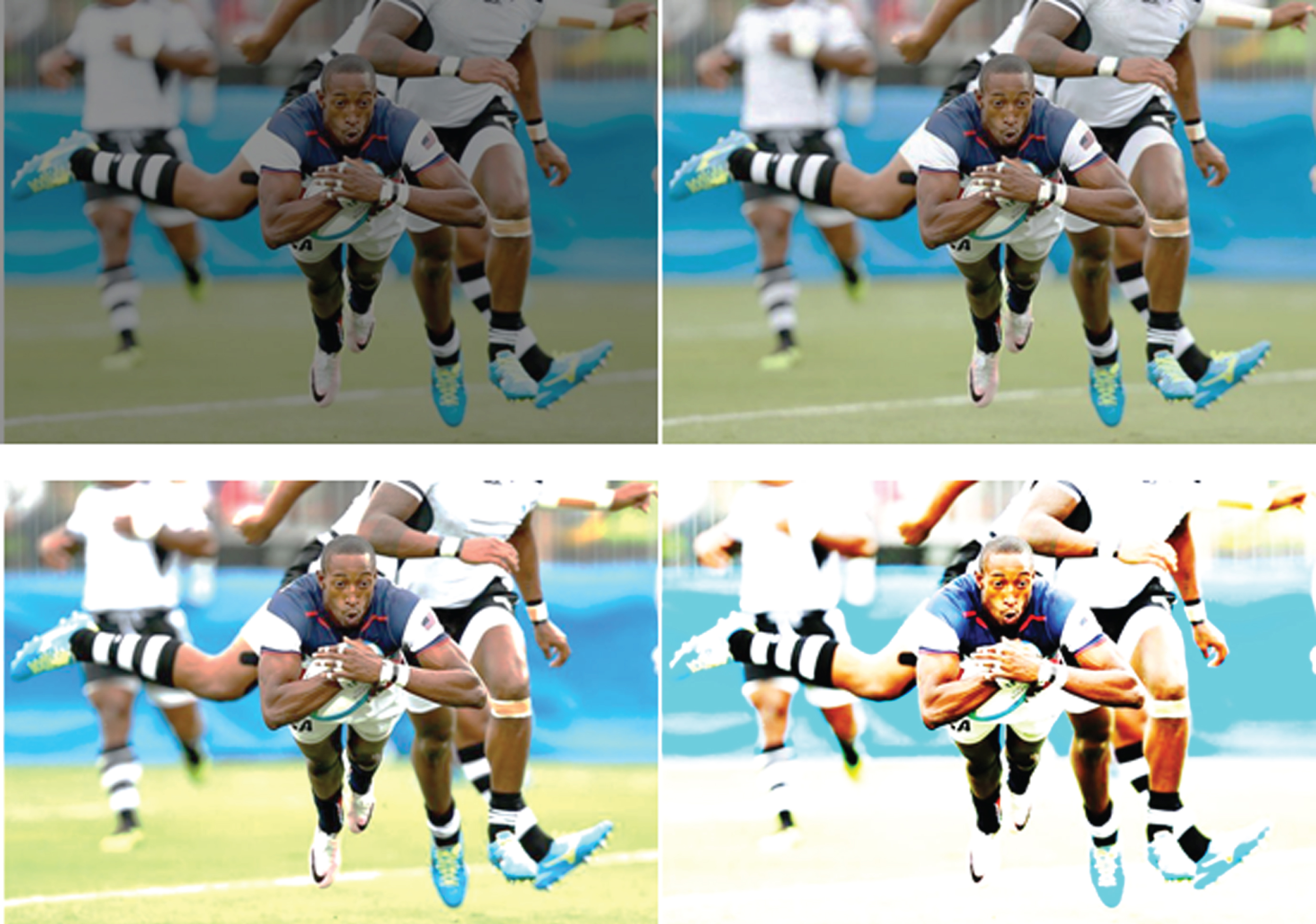
Image data captured at the game site.
Figure 8 shows the recognition results of the image system modeling, which is a data file identifiable by the system. And, through this process, the data is transformed into a data language that the system can recognize. After that, background elimination can be taken on this basis, and feature extraction is performed on the image, and the obtained result is shown in Fig. 9.

Intelligent modeling and recognition of images.
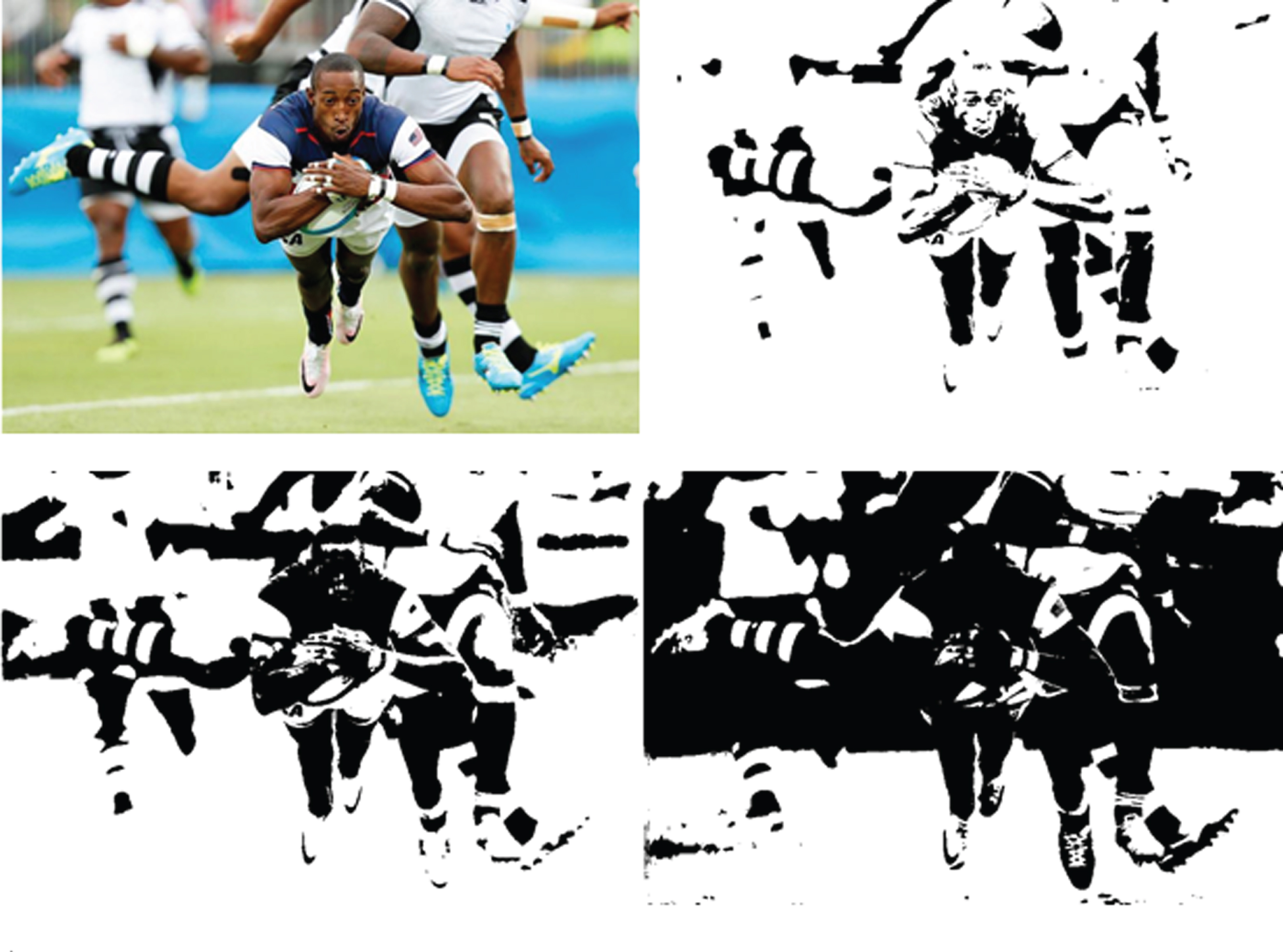
Feature recognition results.
The feature recognition result is shown in Fig. 9, and the image of the player is subjected to motion recognition of a plurality of modes. In order to verify the accuracy of the research model, 10 sets of sports actions were set to judge the accuracy of the action. The results are shown in Table 3.
Verification analysis of algorithm model performance
As shown in Table 3, the algorithm model of this study is compared with the traditional algorithm model. In the Table 1 indicates correct recognition and 0 indicates recognition error. From the results in the table, it can be seen that the traditional algorithm has some shortcomings in the recognition accuracy. However, the algorithm of this study can accurately identify 10 actions. It can be seen that the algorithm of this study has higher recognition accuracy. After that, the recognition speed of the model algorithm is compared, and the obtained result is shown in Fig. 10.

Comparison of model recognition speed.
As shown in Fig. 10, the algorithm model of this study is much faster than the traditional algorithm model in the speed of sports feature recognition.
Through the above comparative analysis, it can be seen that the proposed algorithm is higher than the traditional algorithm in recognition accuracy and recognition speed, so the research algorithm can be applied to sports feature recognition.
This paper first introduces the important application of texture extraction in image processing and analyzes four common texture feature extraction methods: statistical method, model method, structure method and signal processing method. Then, this paper introduces the development of wavelet transform to multi-scale geometric analysis and discusses the theory and implementation process of Contourlet transform and NSCT. In introducing texture recognition, this study focuses on the advantages of SVM theory. Moreover, this study combines the non-subsampled Contourlet transform and the support vector machine to simulate the image of the Brodatz texture library to find the optimal feature vector group that can best characterize the image texture. After that, this study uses this feature to classify and identify sports feature recognition, which further promoted the application of frequency domain analysis and feature recognition theory of support vector machine in practice and the development of computer-aided diagnosis. In addition, this study studies the extraction method of texture features and deeply analyzes the principle of non-subsampled Contourlet transform. At the same time, this study uses NSCT to transform the image from the spatial domain to the frequency domain and extracts the texture features of the decomposed low frequency sub-band, intermediate frequency sub-band and high frequency sub-band image respectively. Preferably, this study selects the appropriate parameters to establish the support vector machine model and applies the extracted texture features into the support vector machine for identification, and selects the features that can best characterize the image texture.
Footnotes
Acknowledgment
This paper was supported by (1) Young Scholars Program of Shandong University (2018WLJH16); (2) Laboratory Construction and Management Funds of Shandong University (SY20193202).