
Abstract
Most of the current plans for Alzheimer’s interventions to improve nursing interventions for patients are designed by clinical nurses themselves, which lack a theoretical basis and are not professional enough. Moreover, cognitive training only addresses a single aspect of rehabilitation for patients with cognitive dysfunction, so it lacks integrity. This study combines MRI and image recognition segmentation technology, adopts multi-party combined interventions for nursing rehabilitation, and uses image recognition technology to conduct experimental research. In addition, this study uses a team of doctors, nurses, and rehabilitators to form a team therapy model, which actively echoes the concept of multidisciplinary cooperation and has a solid medical and theoretical basis. The results show that occupational therapy has a significant effect on slowing the deterioration of patients’ cognitive function, improving their daily living ability, and ultimately improving the quality of life of patients.
Introduction
Alzheimer’s is a very important cause of functional disability in the elderly. According to data published in the World Alzheimer’s Disease Report 2016 [1], there were approximately 9.9 million new cases of Alzheimer’s disease worldwide in 2015, with an average of 1 case every 3 seconds. It is estimated that by the middle of this century, the number of cases of Alzheimer’s worldwide will increase from 46.8 million in 2015 to 13.15 million. Among patients with Alzheimer’s disease, the proportion of those with a clear diagnosis is very small. In low- and middle-income developing countries and middle-income developed countries, fewer than 10% of their patients are diagnosed. Moreover, less than half of the patients in high-income developed countries have a clear diagnosis. The cost of treating Alzheimer’s is very high. The cost of treating Alzheimer’s in the United States alone is as high as US $ 818 billion, and the related costs are expected to increase to US $ 1 trillion next year, and its cost will reach US $ 2 trillion by 2030. In the two decades from 1990 to 2010, the number of cases of Alzheimer’s has doubled on average every ten years. There were about 36 million cases of Alzheimer’s disease worldwide in 2010, of which about 9 million were in China, accounting for 1/4 of the total [2]. Moreover, the number of cases of Alzheimer’s in China accounts for about one third of the total number of cases worldwide. In the next 50 years, with the aging of China’s population, the number of cases of Alzheimer’s will increase dramatically, which will become a serious social and public health problem in China [3].
At present, there is no clinically proven drug that can reverse or stop the progression of the disease. Therefore, the limitations of pharmacological treatment underscore the importance of non-drug interventions. In recent years, a variety of non-drug interventions have been explored at home and abroad, and various intervention measures have emerged endlessly, and some positive progress has been made.
Related work
Through further research, we found that: the nursing intervention [4] schemes are mostly designed by clinical nurses, which lack theoretical foundation and are not professional. Cognitive training [5] only deals with a single aspect of rehabilitation for patients with cognitive dysfunction, so it lacks integrity. In behavior exercise [6], patients only passively receive intensive training and ignore the patient’s self-experience, so it is difficult to improve the patient’s enthusiasm.
Multi-sensory stimulus was first proposed by the Dutch in the late 1980 s, and it quickly gained attention in Europe and later developed into the United States and Canada. Through the use of gentle music, light, touch, fragrance, and thematic visual dynamic projection effects, patients’ anxiety is relieved, social behavior is improved, and the sense of rejection for treatment is resolved. Jong Eun Park [7] randomly divided AD patients into aromatherapy group, aromatherapy + massage group and control group to take intervention treatment for 4 weeks. In addition, he compared the changes in aggression behavior, emotional response and exposure of patients before the intervention, 1 week after the intervention and 3 weeks after the intervention. However, in the study of Tomasz Wichur [8], aromatherapy and massage were also used to treat sensory stimulation of Alzheimer’s patients twice a day for 6 weeks, and it was found that the patients’ mood and agitation behavior were not improved. The researchers analyzed that this may be related to the patient’s olfactory dysfunction. The incidence of olfactory dysfunction is high in patients with dementia, especially in patients with Lewy body dementia [9].
Commonly used exercise therapies include casual exercise, relaxation exercise, endurance exercise and overall exercise, such as various medical gymnastics, medical walking, aerobic exercise, Tai Chi, etc. n the study of Guo-De Wu [10], directional exercise therapy was used, and 117 patients with Alzheimer’s disease were specifically designed and implemented by professional sports therapists and occupational therapists. Similarly, Ningning Zhao [11] randomly divided 74 patients with mild to moderate senile dementia into a personalized function-enhancing activity group and a general activity group.
When performing occupational therapy, some soothing and beautiful music is appropriately played to relax the patient’s mood and create a beautiful atmosphere. For example, David Mengel [12] combined music with calligraphy, painting and other multi-party joint intervention methods, which not only effectively improved the enthusiasm and initiative of patients to participate in activities, alleviate their apathy symptoms, but also increased the joy and comfort of the work experience.
Commonly used methods include transcutaneous electrical nerve stimulation, light therapy, magnetic stimulation, conductive heat therapy, and cold therapy. Research by Hashmi Waleed Javed et al. [13] confirmed that repeated transcranial magnetic stimulation (rTMS) can effectively improve cognitive function in patients with mild to moderate AD. In particular, the effects of high-frequency rTMS interventions are more pronounced. However, Bercovitz Anita [14] performed transcranial direct current stimulation (tDCS) treatments on 20 patients with moderate AD within 2 weeks and evaluated the effects in the first and second weeks and 1 week after the end of treatment. In addition to the above, non-pharmacological intervention methods for AD patients include environmental therapy, pet therapy, acupuncture and acupressure, etc., but these methods are not widely used in clinical practice, especially for the intervention of apathetic symptoms [15]. The development of an intervention plan should be based on the actual situation of the patient, such as the degree of illness, self-care ability and hobbies. At the same time, we should pay attention to the participation of caregivers, strengthen the health education of caregivers, enrich the knowledge of dementia, and avoid the negative impact of the wrong behavior of patients.
Categorical principal component analysis
For n number of measurement data, each measurement data has p variables X1, X2, …, X
p
., that is, the original data matrix is:
When all variables in the data set are numerical and linearly correled, the output of PCA and NLPCA will be the same. When the variables analyzed are nominal or ordinal, NLPCA will be treated as a non-linear relationship. The variables in this study have both numerical and nominal variables, so we use Categorical Principal Components Analysis (CATPCA) in NLPCA to process the data. The function of this method is the same as the principal component analysis for use and standard. For categorical data, it will first convert the original data into optimized data and uniformly convert it into quantitative scores, so that it can be applied to any type of data. Moreover, it does not place any requirements on the type of distribution that the variable obeys [16].
Analysis steps of CATPCA:
(1) Univariate data check
The first step in the data analysis process is to perform a univariate check on the original data. Although CATPCA does not make assumptions about the distribution of the variables, and the deviation of the distribution itself is not a problem, variables with lower frequencies may cause instability in the CATPCA solution or may have a greater impact on the quantification process.
(2) Specify preliminary analysis options
The second step of the analysis process is to perform a multivariate test on the original data. For each variable in the data set, the researcher can set the optimal measurement level and weight for the analysis variable. In CATPCA, strong correlations between analysis variables are not a problem.
Determination of the best measurement level and weight
In order to obtain comparable results, after the data is processed by linear PCA or factor analysis, we need to quantify the data according to the vector model and choose a nominal zoom level. The purpose is not to exclude monotonic or non-monotonic nonlinear relationships between variables. In addition, there are many categories of variables that can be splined. Therefore, we first need to specify the optimal metric level and the spline (that is, the number of internal nodes, which is set to 2 by default, indicating that the data is divided into three intervals) and spline analysis level for all variables in the data set (which is set to 2 by default, indicating that the function of each data interval estimation is quadratic). The best measurement levels include: (a) Ordered splines: the category order of the observed variables is stored in the optimally scaled variables. The category points will be on a straight line (vector) passing through the origin. The resulting transformation is a smooth monotonic piecewise polynomial of a selected degree. These segments are specified by the number of internal nodes and the position determined by the process specified by the researcher. (b) Nominal splines. The only information among the observed variables that remains in the optimally scaled variable is the grouping of objects in the category. The order of the categories of the observed variables is not preserved. The category points will be on a straight line (vector) passing through the origin. The resulting transformation is a smooth, possibly non-monotonic piecewise polynomial of a selected degree. These segments are specified by the number and process-determined locations specified by the researchers of the internal nodes. (c) Multi-calibration. The only information among the observed variables that remains in the optimally scaled variable is the grouping of objects in the category. The order of the categories of the observed variables is not preserved. The category points will be in the centroid of the objects in a category. (d) Orderly. The order of the observed variables is stored in the optimally scaled variables. The category points will be on a straight line (vector) passing through the origin. The resulting transformation fits better than the ordered spline transformation, but its smoothness is lower. (e) Nominal. The only information among the observed variables that remains in the optimally scaled variable is the grouping of objects in the category. The order of the categories of the observed variables is not preserved. The category points will be on a straight line (vector) passing through the origin. The resulting transformation fits better than the spline nominal transformation, but its smoothness is lower. (f) Numerical. Categories are ordered and equally spaced (interval degrees). The category order of the observed variables and the equidistance between the category numbers remain in the optimally scaled variables. The category points will be on a straight line (vector) passing through the origin. When all variables are numerical, the analysis is like standard principal component analysis. Variable weights can define weights for each variable. The weight value specified must be a positive integer and the default value is 1 [17].
➁ Treatment of missing values
Unlike the linear PCA calculation process, the CATPCA calculation process is not based on the correlation matrix, but on the data itself. Therefore, the handling of missing values is more complicated than linear PCA. Linear PCA only needs to simply exclude cells in a data matrix containing missing values, without the need for pairwise or list deletes. This treatment of missing values is called a passive processing variable in CATPCA and is the default option. The advantage of using passive processing is that all available data is used for analysis without the need to “populate” additional data. In order to find out whether individuals with missing values are different from other individuals, the deletions can also be included as additional categories in CATPCA. The level of analysis, which is independent of the variables, and the missing categories will get an optimal nominal quantification. If this quantification is significantly different from other quantifications, it indicates that the missing individual is a special group and is not comparable to other individuals. When missing values occur randomly, there is only a slight difference between passive handling of missing and treating missing as an additional category [18]. CATPCA treats 0 as a missing value. If there is a 0 in the original data, it needs to be re-encoded or discretized.
➂ Discretization
CATPCA requires (positive) integer-valued data, which is a technical requirement and not a requirement inherent to the CATPCA method. Unless otherwise specified, fractional variables are grouped into seven categories with approximately normal distributions (if the number of different values of the variable is less than seven, the categories are divided by this number). Discretization methods include: (a) Grouping. This step re-encodes a specified number of categories or re-encodes by interval. (b) Rank. This step discretizes the variables by ranking the cases. (c) Multiply. The current value of the variable is a normalized value that is multiplied by 10 and rounded, and it adds a constant to make the lowest discrete value be 1[19].
➃ Determination of the principal component dimension
In linear PCA, the principal component dimension used in the analysis is only related to the interpretation of the results, and the CAPTCA principal component dimension affects the analysis results [20]. The reason is that the eigenvalues of the first principal component will be maximized by optimal scaling. For example, the two principal components of a two-dimensional principal component analysis result are not the same as the first two principal components of a three-dimensional principal component analysis result. Therefore, when choosing the principal component dimension, the results of different dimensions should be compared.
(3) Analysis and adjustment of options
Normalization methods can normalize object scores and variables, and only one normalization method can be used in each analysis. It can specify any real number in the interval [–1,1]. A value of 1 is equivalent to the Primary Object method, a value of 0 is equivalent to the Symmetric method, and a value of –1 is equivalent to the Primary Variable method. By specifying values greater than –1 and less than 1, we can distribute eigenvalues across objects and variables.
□Var (F) is the most important indicator for the quantification of principal components and variables, so it is used as the main criterion for variable selection. Var (F) is composed of the main components of each variable and is represented by the characteristic value λ. The principal component contribution rate is the ratio of the principal component variance Var (F) to the total sample variance, that is, the ratio of a feature value to the total feature value. This indicator represents the proportion of the original component carrying the primary data information.
Then, the contribution rate of the ith principal component is:
The cumulative variance contribution rate is:
(4) Determine analysis results and interpretation
Step (3) of the above process can be repeated multiple times until a reasonable result is obtained. Moreover, it can be interpreted according to the actual situation of the data to get the final conclusions about the original data.
According to the requirements of the sample size formula, the QOL-AD scale with the most entries in the evaluation index was selected, and the average values of the total QOL-AD scores of the two groups were 34.87 points and 35.44 points, and the standard deviations were 4.29 points and 3.94, respectively. The data was substituted into the PASS11 software and calculated using two independent sample mean formulas. We set α= 0.05 and β= 0.1 and obtained a sample size of 34 cases in each group, and 68 cases in both groups. Considering the special circumstances such as the possibility of the patient’s withdrawal or discharge, based on a sample loss rate of 15%, a total sample size of at least 78.2 cases is required in each group, and 39.1 cases in each group. Therefore, the sample size was determined to be 80 in this study [21]. The study uses a simple lottery method for random grouping. Before the grouping, a non-transparent closed carton was prepared. The paper strips with 1–80 digits were folded and placed in the box. The researcher was responsible for uniformly drawing lots of eligible subjects. Those who were singular entered the control group, and those who drew even numbers entered the intervention group.
This study is a randomized controlled trial.
(1) Set up an occupational therapy team: The head of the psychiatric psychiatrist team serves as the team leader. The psychiatric nurse (with at least 2 years of psychiatric work experience) is the main member. The geriatric psychiatrist and rehabilitator pticipate in cooperation to jointly design an occupational treatment program for Apatients. (2) Research object: From August 2017 to June 2018, patients with mild to moderate AD in geriatric psychiatry in a tertiary specialist hospital were selected. Researchers need to explain the research content to patients and their families, obtain consent, and sign informed consent. (3) Pre-test: Twenty AD patients who met the criteria were randomly divided into intervention group and controlroup, with 10 in each group. A two-week pre-experiment was performed to adjust the details of the treatment plan and calculate the sample size. (4) Grouping: The selected research subjects were randomly divided into intervention group and control group. 5) Intervention: The control group was given conventional care, and the intervention group was given a multi-party combined intervention method based on conventional care. The intervention time was 6 months. (6) Efficacy evaluation: Alzheimer’s Cognitive Rating Scale, Modified Barthel Index Scale, and Modified Quality of Life Scale for Alzheimer’s Disease were used at the end of 1 month, 3 months, and 6 months after intervention to assess the efficacy of the two groups of patients.
T control group performed routine nursing care, including: executing doctor’s orders, daily life care, health education, assisting in walking, watching TV, electroencephalography, biomimetic electrical stimulation treatment, psychological nursing, and diet nursing.
The intervention group added multi-party combined intervention treatment on the basis of giving routine care. According to the characteristics of the research object is the elderly, the selected activities need to be safe and easy for the elderly to accept, and combined with the patient’s hobbies, specialties and needs.
Test results
The mixed effects model analysis of repeated measurement data was used to compare the changes in cognitive function between the two groups before, at the end of 1 month, at the end of 3 months, and at the end of 6 months. The results showed that the cognitive function of the intervention group was statistically different from that of the control group (F = 5.26, P < 0.05). The difference in cognitive function between the two groups of patients was statistically significant over time (F = 167.71, P < 0.05), and there was an interaction between time and group factors (F = 29.53, P < 0.05). The detailed information is shown in Table 1. The cognitive function of the two groups showed the same at baseline, and there was no statistical difference (P > 0.05). At the end of the first month, there was no statistical difference in cognitive function between the two groups (P > 0.05). At the end of the 3rd month and the end of the 6th month, the cognitive function of the two groups was statistically different (P < 0.05), and the cognitive function of the intervention group was better than that of the control group, as shown in Table 1. In addition, from the longitudinal development trends of the two groups, it can be found that the ADAS-cog scores of both groups of patients show an upward trend, but the increase in the intervention group is significantly lower than that in the control group, as shown in Fig. 1. Compared with the baseline, the mean difference at the end of the 6th month of cognitive function in the intervention group was –2.80, showing a statistical difference from the baseline (P < 0.05). The mean differences at the end of 1 month and 3 months were –0.38 and –0.52, respectively, and these two time points were not statistically different from the baseline (P > 0.05). Figure 2 shows that the cognitive function of patients in the intervention group remained basically at the same level during this period. The cognitive function of patients in the control group decreased significantly. The mean difference from baseline at the end of 1 month was –0.57, and the difference was not statistically significant (P > 0.05). The mean difference between the end of 3 months and the end of 6 months and the baseline was –3.23, –7.36, which had statistical differences (P < 0.05). Moreover, as time goes on, the negative change of this difference will become larger, as shown in Table 1.
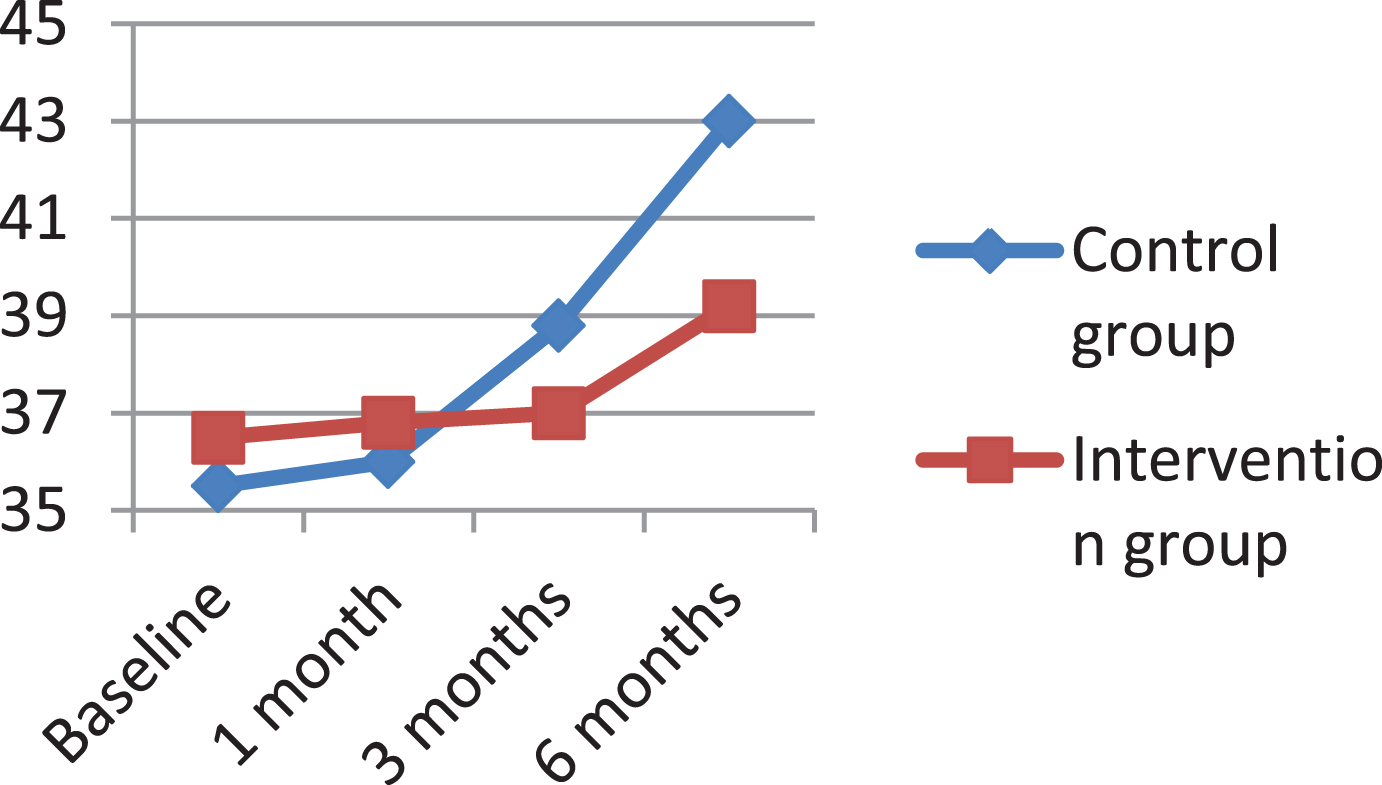
Trends in cognitive function in each time period in the two groups.
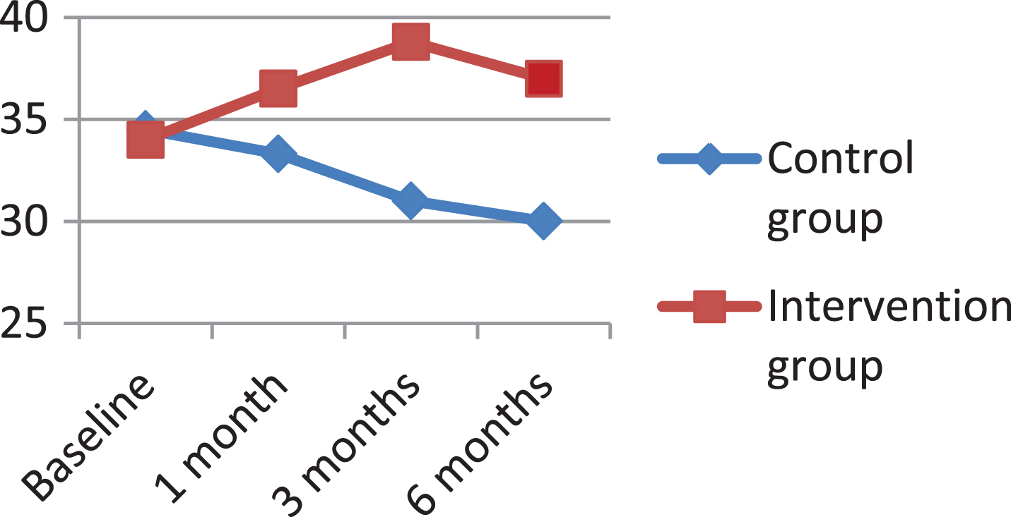
Trends in the quality of life in the two groups at different time periods.
Comparison of daily living ability between two groups and baselines after intervention
The mixed effects model analysis of repeated measurement data was used to compare the changes in quality of life between the two groups before, at the end of 1 month, at the end of 3 months, and at the end of 6 months. The results showed that the quality of life of patients in the intervention group was statistically different from that of the control group (F = 23.25, P < 0.05). The quality of life of the two groups of patients was statistically different over time (F = 5.91, P < 0.05), and there was an interaction between the two factors of time and group (F = 19.94, P < 0.05), as shown in Table 1. The two groups of patients showed consistent quality of life at baseline, and there was no statistical difference (P > 0.05). There were statistical differences at the end of the first month, the third month, and the sixth month after the intervention (P < 0.05), and the quality of life of the intervention group was significantly better than that of the control group. See Table 2 for details, as shown in Table 1. From the longitudinal development trends of the two groups, it can be found that the QOL-AD scores of the two groups of patients show opposite development trends over time, as shown in Fig. 1. The intervention group showed an upward trend, and the curve decreased slightly at the end of the 6th month. Compared with the baseline, the mean differences at the end of the first month, the end of the third month, and the end of the sixth month were 2.55, 4.75, and 3.11, and there were statistical differences between the three time points and the baseline (P < 0.05). However, the control group showed a downward trend. The mean difference from baseline at the end of the first month was –1.06, which was not statistically different (P > 0.05). The mean differences at the end of the 3rd month and the end of the 6th month were –3.48 and –4.46, respectively, which were statistically different from the baseline (P < 0.05). as shown in Table 2.
Comparison of the quality of life between the two groups and the time period after the intervention with the baseline
In this paper, the size of all the images used is normalized to 256×256×186, and the three-level resolution registration method is used. The sampling interval is 2×2×2, and the highest resolution is the original image resolution. The second level resolution is 128×128×93, and the third level is sampled based on the second level, and the resolution becomes 64×64×46. The genetic algorithm is used as the optimization algorithm in the search process, and the mutual information is used as Similarity measure, the interpolation algorithm uses trilinear interpolation, resolution iterations at all levels are 50 times, and the coarse-to-fine registration is performed at the 3-level sampling rate to obtain the optimal transformation parameters. In order to verify the effectiveness of the algorithm, we perform a rigid body transformation on an image in the sample, and the translation amount on the xyz axis is (10,15,0) and 3 rotation angles (10,0,0) to generate the image to be registered. Figure 3 (a), (b) show the same slice in the original image and the image to be registered.

Reference image and image to be registered after rigid body transformation.
For the binarized image, calculate the center of gravity of the brain tissue as the center of the initialization level set, calculate the distance from the center of the circle to each point on the boundary between the brain region and the non-brain region of the binarized image, and take the statistical average value as the brain The radius of the area. Use this circle with its center and radius as the initial value of the level set. Figure 4 shows a brain image slice that determines the initial value of the level set.

Brain image of the initial value of the level set.
When performing skull stripping on a 3D MR brain image, we can use the fitted level set curve of the current slice as the initial contour of its adjacent slices. This not only saves computing time, but also enables the continuity of contours between adjacent slices. And smoothness, but also improve the accuracy of the results. Therefore, we generally choose the middle slice of the head for the initial slice selection, which can better reflect the outline of the complete brain tissue than the top and bottom ends of the head. In order to ensure that the initial contour curve of the next slice of the current slice is inside the brain tissue, we uniformly shrink the fit curve of the current slice to the inside by 2 mm as the initialization curve of the next slice, and so on. When all two-dimensional slices After all processing, a three-dimensional image of the skull after peeling is obtained. As shown in Figs. 5 and 6.

Three-dimensional view before peeling.

3D image after peeling.
Figure 7 is an analysis and observation chart of the research problem. Figures a and c are brain magnetic resonance images of two groups of patients from the same layer. It cannot be observed from the images whether there is Aβ deposition. Figures b and d show the left hippocampus in the two images, respectively. From this image, it can be found that for the control group, the brain tissue image contains Aβ deposits (brown spots in the figure), while for the intervention group, the images do not contain Aβ deposits. This phenomenon cannot be found by observing the original brain MR images, and it can only be achieved through data post-processing.
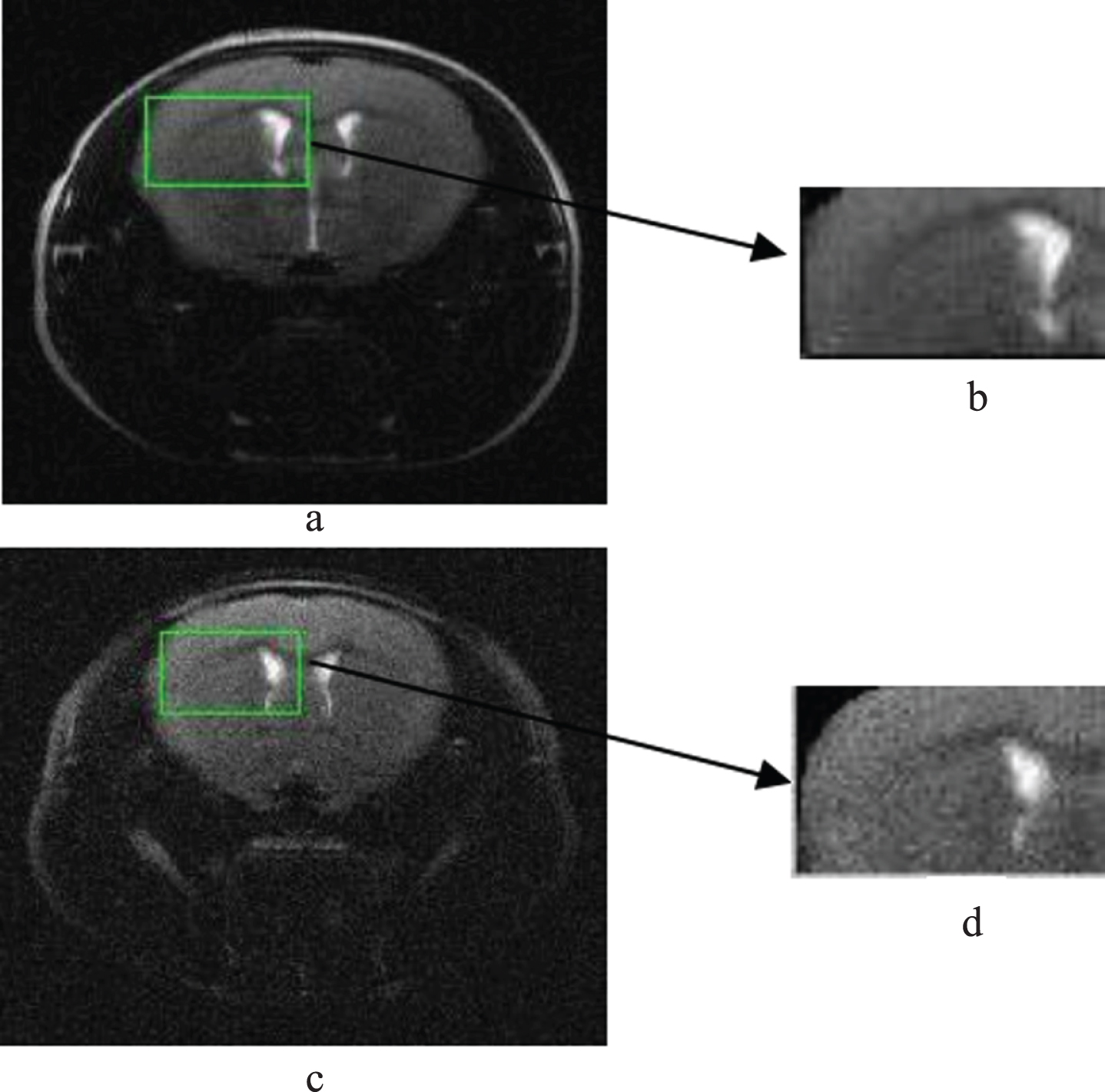
Brain MRIS image.
This paper uses MRIcro software to efficiently view and transform brain MR images, and input and output brain imaging data. Because Aβ deposition is located in the brain tissue region, the brain tissue region is the region of interest (ROI) studied in this paper. This article uses MRIcro to create and save it. In order to ensure the accuracy of segmentation, this article uses MRIcro to manually draw the outline of the brain tissue and perform a filling operation. The ROI is output as an analytical image to obtain the brain tissue image shown in Fig. 8 below.

Brain tissue segmentation effect.
Figure 9 shows the brain area atrophy image of patients with severe cognitive condition, which is like the brain area atrophy image of some patients with severe condition in the control group. In this study, the patients in the intervention group improved significantly after physical therapy with the combined intervention method.

Image of brain atrophy in patients with severe cognitive problems.
This study mainly used a team of doctors, nurses, and rehabilitators to form a team of treatment models, which actively echoed the concept of multidisciplinary cooperation and has a solid medical and theoretical basis. At the same time, the research results show that occupational therapy has a significant effect on slowing the deterioration of patients’ cognitive function, improving their daily living ability, and ultimately improving the quality of life of patients. At the same time, medical personnel can observe the changes of the patient’s condition at any time during the operation to ensure the effectiveness of the treatment and the safety of the patient, which is very beneficial to the treatment and monitoring of the patient. The whole research process shows the feasibility of the implementation of the plan in the hospital, which can be used as a reference for clinical medical staff. The application of multi-party combined intervention can slow the deterioration of cognitive function in patients with Alzheimer’s disease, maintain the daily living ability of patients with Alzheimer’s disease, and significantly improve the quality of life of patients with Alzheimer’s disease. Multi-party combined interventions for nursing rehabilitation has a certain effect on the rehabilitation of AD patients.