Prediction model for stock price trend based on convolution neural network

a) Missing value processing

There are missing values in the original stock trading data. This paper adopts the following methods to deal with missing values: 1. For a training set with a sufficient number of samples, a single piece of data will be directly discarded, that is, when there is a vacancy value in a data record, the corresponding entire data record will be deleted directly; 2. For a test set with a small sample, the mean value filling method is selected., that is, when there is a vacancy value in a data record, the average value of the corresponding variables in the above and below two adjacent days is taken to fill the vacancy value.

b) Data standardization

As can be seen from the basic stock transaction data listed in Table XX, the values of each variable are in different orders of magnitude. Without normalization, the effect of a large number of variables on the result will overwrite the effect of small, leading to the loss of the information contained in the small order variable. Therefore, each variable of the original sample data must be standardized. It should be noted that, because there is a correlation between the opening price, the closing price, the highest price and the lowest price of the variables, these four variables must be standardized. This paper will use min-max standardization:

Min-max normalization method: x i ′ = x i - x min x max - x min(1)

Where x _i is the raw data to be normalized, x _max and x _min represent the maximum and minimum values in the raw data sequence to be normalized, and x i ’ is the target data obtained after min-max normalization, and its value range is [0,1].

c) Define ups and downs labels label = { 1 , Opnprc t + 1 ⩾ Opnprc t 0 , else(2)

Among them, Opnprc _t is the opening price on the tth day. If the opening price Opnprc_t+1 on the t + 1 day is greater than or equal to the opening price Opnprc _t on the t day, then the t day is up and marked as “1”; otherwise, it is “down”. Marked as “0”.

a) Continuous technical indicators-actual time series

The following seven technical indicators are used in this paper: MA, K, D, WR, MACD, RSI, and CCI. According to Table 2, this 7 technical indicator value can be calculated by using the original transaction data, and these 7 technical indicator values are also used as inputs in the prediction model. By observing Table X, it is not difficult to obtain that the technical indicators obtained based on the corresponding formula are also continuous values, and they will be normalized between [–1, 1] to avoid the situation where large orders of magnitude cover small orders of information.

b) The discrete technical indicators-the trend of the indicators

Research [7] pointed out that some technical indicators that can predict the future movement of stocks, so continuous technical indicators are cited in part. The prediction model is based on the existing data to extract valid credits for prediction. This paper proposes to add a new decision-making layer to convert continuous technical indicators into discrete ups and downs through existing expert knowledge and experience. The actual indicator time series sequence calculated by part a is used to determine the stock’s rise and fall based on the characteristics of the indicator data through certain rules. Among them, “+1” represents an increase and “-1” represents a decline. This discrete value reflects the forecast of stocks’ rises and falls based on the existing expert knowledge from this indicator. The following will introduce in detail the expert experience rules for the judgment of the fluctuation of each discrete indicator data.

The Moving average (MA)

The Moving average, which is obtained by averaging the closing prices of stocks (indexes) within a certain period. The averages of different times of stock are connected to form an MA, which is used to observe the trend of stock changes. According to expert experience: if the current price is higher than its moving average, it will generate a buying signal, which indicates that the future market is bullish; if the current price is lower than its moving average, it will generate a sell signal, which indicates that the future market is bearish. Therefore, the following provisions are made: If the current closing price Clsprc is higher than MA, the market’s trend is “up” and marked as “+1”; if the previous closing price Clsprc is lower than MA, the market’s trend is “down”, marking Is “-1”. There are five-day, 10-day, 30-day, 60-day, 120-day, and 240-day indicators in the stock market. This article uses the 10-day moving average, which is MA2.

Stochastic indicators K, D

K and D use the fluctuations of the highest price, the lowest price, and the closing price in the past few trading days to estimate the future stock price fluctuation trend, which can accurately reflect the random amplitude of the stock over a period, so they are good technical indicators for short-term trend band analysis and judgment. Some experts pointed out: Generally when the KDJ values of the month are low, it will gradually enter the market to absorb, which will generate a purchase signal. Therefore, the following provisions are made: if the current K value is greater than the previous day’s K value, the market’s trend is “up” and marked “+1”; if the current K value is less than the previous day’s K value, the market’s trend is “down”, marked as “-1”. Also, D complies with this requirement.

William Index (WR)

The highest, lowest, and closing prices of the “last cycle” can be used to calculate the swing point of the closing price of the day, to determine whether the market is overbought or oversold. Some experts have pointed out that WR is a swinging reverse indicator, that is, when the stock price rises, the WR indicator goes down; when the stock price falls, the WR indicator goes up. Therefore, the following provisions are made: if the current WR value is less than the previous day’s WR value, the market’s trend is “up” and marked as “+1”; if the current WR value is greater than the previous day’s WR value, the market’s trend is “down”, marked as “-1”. WR1 is a 10-day trading strength indicator; WR2 is a 6-day trading strength indicator. This paper uses WR1.

Exponential Smoothing Moving Average (MACD)

MACD is obtained by subtracting the slow exponential moving average (EMA26) from the fast exponential moving average (EMA12). Some experts point out that when MACD changes from negative to positive, it is a signal of purchase. When MACD changes from positive to negative, it is a signal to sell. Therefore, the following provisions are made: if the current MACD value is greater than the previous day ’s MACD value, the market’s trend is “up” and marked as “1”; if the current MACD value is less than the previous day ’s MACD, the market’s trend is “down” marked “-1”.

Relative Strength Index (RSI)

The relative strength index (RSI) is a numerical calculation to quantitatively analyze the market’s trading intention and strength. The relative strength index RSI believes that in a normal stock market, the stock price can be stable only when the strength of long and short sellers and buyers must be balanced. Some experts point out that the value range of the RSI indicator is between 0 and 100. Above 70 can be considered overbought and below 30 can be considered oversold. In the normal (30, 70) interval, if the upward force is large, the RSI curve rises and it is a signal to buy; if the downward force is large, the RSI curve is down and it is a signal to sell. Therefore, the following provisions are made: if the current RSI value is less than 30, the market’s trend is “up” and marked as “+1”; if the current RSI value is greater than 70, the market’s trend is “down” and marked as “-1 “; If the RSI value is between 30 and 70, the current RSI value is greater than the previous day’s RSI value, the market’s trend is” up “, marked as”+1 “, the current RSI value is less than the previous day RSI value, the market’s trend is up “Down” and marked “-1”.

Commodity Channel Index (CCI)

CCI is an indicator that specifically measures whether the stock price has exceeded the normal distribution range and fluctuated between positive infinity and negative infinity. Some experts point out that over 100 can be considered overbought, and below 100 can be considered oversold. In the shock zone (-100,+100), if the upward force is large, it is a signal to buy; if the downward force is large, it is a signal to sell. Therefore, the following provisions are made: if the current CCI value is less than -100, the market’s trend is “up” and marked as “+1”; if the current CCI value is greater than 100, the market’s trend is “down” and marked as “- 1 “; if the CCI value is between -100 and+100, the current CCI value is greater than the previous day’s CCI value, the market’s trend is” up “, marked as”+1 “, the current CCI value is less than the previous day’s CCI value, the market’s trend is “down” and marked as “-1”.

The input of the prediction model includes two parts: basic transaction data and technical indicator data. The output of the prediction model is the ups and downs prediction label, which adjusts our model by comparing the results predicted by the model with the actual ups and downs. Among them, this research will use two methods to represent technical indicator data. The first method is to use the time series of actual technical indicators calculated based on the basic transaction data of each stock, that is, continuous type; the second method is to obtain the trend of each indicator through the experience of relevant experts, that is, the discrete type. Discrete technical indicators refer to the use of existing expert experience to obtain effective stock trend information from actual technical indicator data. When the discrete technical indicator data is directly used as the input of the model instead of the actual continuous value, the trend information perceived by each technical indicator has been input to the model. Compared to the method of directly inputting the original indicators for stock price fluctuation prediction, this is a step forward in a sense. Subsequent experimental sections will discuss whether the use of discrete technical indicator data as input to the model is more effective than actual continuous values.

3.1 The prediction model design based on convolutional neural network (CNN-M)

In this section, the prediction model of the stock price trend based on the convolutional neural network constructed in this paper is shown in Fig. 1. The structure is divided into the following seven layers: an input layer, five hidden layers, and an output layer.

OPEN IN VIEWER

Fig. 1

The prediction model based on convolutional neural network.

Input layer: which is accept two-dimensional stock image samples. This paper uses the data of the previous T trading days to predict the stock price change on the (T + 1)th day, and the dimension of the stock data feature set is 20, 6 basic market indicators plus 14 stock technical indicators. Therefore, the dimension of the data accepted by the input layer is [T×20]. In this experiment, the time window size is 20. Therefore, the 2D image sample size specification for stock data is [20 * 20].

Convolution layer 1(Conv1): Use 64 3 * 3 size filters to extract 2D stock image features for convolution operations. The horizontal and vertical sliding window steps are both 1. The padding method uses “SAME” to keep the picture size unchanged. Therefore, after the convolutional layer 1 operation, the matrix size becomes: [20 * 20 * 64].

Convolution layer 2(Conv2): Use 128 3 * 3 size filters to extract image features and perform convolution operations. The sliding window has a step size of 1. The padding method uses “SAME” to keep the picture size unchanged. Therefore, after the conv2 operation of the convolutional layer, the matrix size becomes: [20 * 20 * 128].

Pooling layer: The maximum pooling method is used. The horizontal and vertical sliding window steps are both 2. The padding method uses “SAME”. Through the pooling operation, the output matrix size is reduced by half in both the horizontal and vertical directions. Therefore, after the convolution layer pooling operation, the matrix size becomes: [10 * 10 * 128].

Fully connected layer 1(Fc1) and fully connected layer 2(Fc2): Set 256 and 64 neurons respectively, and set Dropout = 0.5.

Output layer: Use Softmax to implement ups and downs classification.

See Table 3 for specific network parameters.

In this section, the prediction model of the stock price trend based on the residual neural network constructed in this paper. At present, only the superposed two-layer residual module is considered, and the superposed multi-layer residual module will be analyzed in Experiment 5.5.2. As shown in Fig. 2, the model is divided into the following layers:

OPEN IN VIEWER

Fig. 2

Structure of prediction model based on residual network.

Input layer: which is accept two-dimensional stock image samples. As this paper uses the data of the previous T trading days to predict the stock price change on the (T + 1)th day, and the dimension of the stock data feature set is 20, 6 basic market indicators plus 14 stock technical indicators. Therefore, the dimension of the data accepted by the input layer is [T×20]. In this experiment, the time window size is 20. Therefore, the sample size of the two-dimensional stock image for stock closing is [20 * 20].

Convolution layer 1: Use 64 3 * 3 size filters to extract two-dimensional stock image features and perform convolution operations. The horizontal and vertical sliding window steps are both 1. The padding method uses “SAME” to keep the picture size unchanged. Therefore, after the convolutional layer 1 operation, the matrix size becomes: [20 * 20 * 64].

Residual module layer: The residual module uses the Bottleneck structure, which can be stacked by one or more Bottleneck. Bottleneck’s internal structure is shown in 4.X, which consists of three convolutional layers. The function of the convolutional layer 1 is to reduce the dimension; the feature of the convolutional layer 2 is to extract the feature without any change in the dimension; the function of the third layer is to increase the dimension and return the dimension to the original dimension. By this method, one function is to increase the number of network layers (from two to three layers), and the second function is to greatly reduce the parameter amount. To improve the model learning rate and performance.

Pooling layer: The maximum pooling method is used. The horizontal and vertical sliding window steps are both 2. The padding method uses “SAME”. Through the pooling operation, the output matrix size is reduced by half in both the horizontal and vertical directions.

Fully connected layers 1 and Fully connected layers 2: Set 256 and 64 neurons respectively and set Dropout = 0.5.

Output layer: Use Softmax to implement ups and downs classification.

Taking the stacked two-layer Bottleneck residual module as an example. See Table 4 for specific network parameters.

Step 5: Experiment and analysis. A total of two experiments are proposed in this section. In the first experiment, the research will explore the performance differences between CNN-M and Resnet-M; In the second experiment, the research will explore the impact of network layers on CNN-M and Resnet-M.

4.1 Contrast experiment setting

In the first experiment, the research will explore the performance difference between CNN-M and Resnet-M. CNN-M’s network structure uses a seven-layer CNN model designed in section 3.1, with five hidden layers, two convolutional layers, a pooling layer, and two fully connected layers. The Resnet-M’s network structure uses a prediction model based on the residual network designed in Section 3.2 and uses two layers of Bottleneck stacking.

In the second experiment, the research will explore the impact of network layers on the Resnet-M. In theory, the more layers of convolutional layers, that is, the deeper the neural network, the stronger the ability to extract features. However, deepening the network structure will slow down the learning rate of the model, and the amount of data in this article is relatively small. Deeper neural networks will not necessarily achieve better results. Therefore, based on the 3.2 model, two Bottleneck structures in the original model were stacked to three, four, and five. Explore the impact of network layers on the Resnet-M.

4.2 Two-dimensions sequence samples constructed by sliding window

The input of the convolutional neural network is a sequence of two-dimensional stock image samples (shown in Fig. 3), which converts the one-dimensional sequence of basic stock market data and technical indicator data into two-dimensional stock image data.

OPEN IN VIEWER

Fig. 3

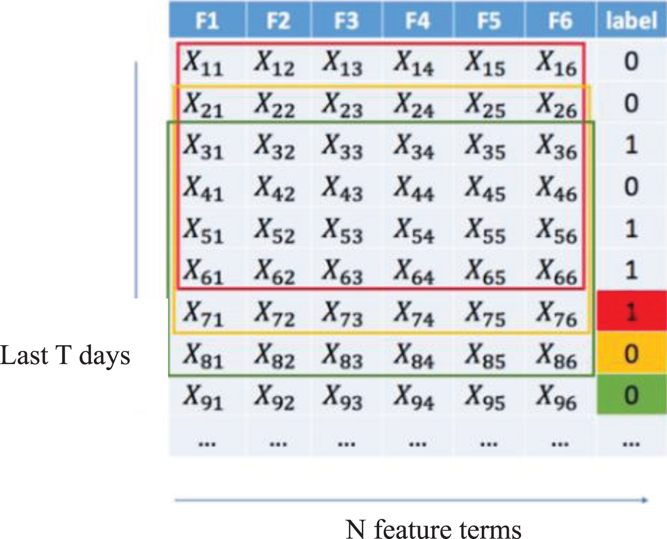
Schematic diagram of constructing a two-dimensional stock image sample (T = 6, N = 6).

The Y-axis represents the specified market data (or technical indicator data) in the past T period sequence and the X-axis represents N market data (or technical indicator data), which is composed of T * N stock picture features input. This is also a two-dimensional stock image sample using a sliding window. Because the data of the previous T days is used to predict the stock price change on the T + 1 day, the input sequence is {x _i , x_i+1, … , x_i+T-1|x _i  = (X_i1, X_i2, … X _in ) }, and the corresponding label is {y_i+T}. Fig. 5 is a schematic diagram generated by a sliding window construction input sequence when the window sizes T and N are 6. The red box is a two-dimensional image sample with 6 * 6 input and the corresponding label is “1” in the red area. A 6×6 input two-dimensional image sample in the next yellow box is obtained through the sliding window and the corresponding label is in the yellow color area “0”. In this way, all two-dimensional stock image inputs and corresponding labels are obtained in order.

OPEN IN VIEWER

Fig. 4

Comparison of CNN-M and Resnet-M prediction results (accuracy & F value).

OPEN IN VIEWER

Fig. 5

The influence of the number of network layers on the Resnet-M (accuracy & F value).

The experimental environment parameters are shown in Table 5.

The experiment uses open-source Tensorflow as a deep learning platform and uses Python 3.5 to write the experimental program. The model hyperparameters are shown in Table 6.

In this experiment, relevant statistical indicators are used to evaluate the predictive performance of the six model stocks that have been set up previously. Evaluation index accuracy (Accuracy) and F value (F-Score) [8]. First, the prediction results of the model will be described. See Table 7 for details.

Before calculating precision and F value, “precision and calling rate” must be obtained first.

The accuracy indicates that in the samples that are predicted to be “up”, the true trend is the proportion of “up”. The recall represents the proportion of samples predicted to be “rising” among the samples whose true trend is “rising”. The calculation formulas are: Precision = TP TP + FP 4(3) Recall = TP TP + FN # 5(4)

Accuracy indicates the proportion of correctly predicted samples to the total sample data. F-Score is the average accuracy and recall. The calculation formulas are:

Accuracy = TP + TN TP + FN + TN + FP # 6(5) F - Score = 2 × Precision × Recall Precision + Recall # 7(6)

The larger the Accuracy and F-Score values, the more predictive the model is.

5.1 Exploring Performance differences between CNN-M and Resnet-M

In this section, the paper will explore the performance differences between CNN-M and Resnet-M. CNN-M’s network structure uses a seven-layer CNN model designed in Section 3.1 with five hidden layers, two convolutional layers, a pooling layer, and two fully connected layers. The Resnet-M’ network structure uses a prediction model based on the residual network designed in Section 3.2 and uses two layers of Bottleneck stacking.

The prediction results of each model are shown in Fig. 4.

It can be seen from Fig. 4 that the prediction accuracy of the ResNet-M reaches 54.8%, while the accuracy of the CNN-M with two convolutional layers is only 52.2%. The ResNet-M in the experiment has 2 Bottleneck structures and each Bottleneck structure has 2 convolutional layers. In other words, the ResNet-M in this experiment, plus the initial convolution operation, has a total of 7 convolutional layers. The accuracy of the ResNet-M is two percentage points higher than the CNN-M, which is expected.

The test results show that the prediction ability of the Resnet-M is better than the CNN-M.

5.2 Exploring the impact of network layers on Resnet-M

In the previous section, the prediction accuracy of the Resnet-M is significantly higher than that of the CNN-M. Therefore, in subsequent research, Resnet-M will be selected for further research and analysis. In this section, the paper will explore the impact of network layers on the Resnet-M. Theoretically, the more layers of the convolutional layer, the deeper the neural network, the stronger the ability to extract features. However, deepening the network structure will slow down the learning rate of the model and the amount of data in this article is relatively small. Deeper neural networks will not necessarily achieve better results. Therefore, based on the 3.2 model, the two Bottleneck structure stacks in the original model are superimposed on 2, 3, 4 and 5 Bottleneck, which are counted as Resnet-2, Resnet-3, Resnet-4, and Resnet-5. Explore the impact of network layers on the Resnet-M.

The prediction results of each model are shown in Fig. 5.

First, in terms of accuracy, Resnet-4 reached 55.9%, followed by Resnet-3, which reached 55.2% and the lowest accuracy was Resnet-2. Resnet-5 performed slightly worse than Resnet-3 and Resnet-4. It is worth mentioning that although Resnet-4 has the highest accuracy rate, it does not perform as well as Resnet-3 in terms of F value. So overall, Resnet-3 performed best in this trial.

The results show that in this experiment, Bottleneck’s superposition of 3 layers is better, not that the deeper the neural network is, the better extract features will be. This is related to the small amount of data in this article and deeper neural networks may not achieve better results.