Integrated MOPSO algorithms for task scheduling in cloud computing

Abstract

Task Scheduling is one of the most challenging problems in cloud computing. It is an NP-Hard and plays an important role in optimizing the use of available resources. Recently, Multi-Objectives Genetic Algorithm (MOGA) is proposed for cloud tasks scheduling. However, the execution time of the GA is higher than Particle Swarm Optimization (PSO), and the convergence is slower. PSO converges fast because it can be implemented without too many parameters and operators. In this paper, Multi-Objectives PSO (MOPSO) and MOPSO with Importance Strategy (IS) (MOPSO_IS) algorithms are proposed. MOPSO algorithm is integrated with the IS to select the global best leader. Furthermore, incorporating a mutation operator in MOPSO_IS resolved the problem of premature convergence to the local Pareto-optimal front. The performance of the proposed algorithms was compared with MOGA and produced better results. The results of the experiments showed that the proposed MOPSO and MOPSO_IS significantly minimized the total task time and average task time and obtained better distribution for tasks on the available resources in a minimal time.

Keywords

Cloud computing load balancing swarm intelligence multi-objectives optimization.

1 Introduction

Cloud computing is recently highlighted as a booming area of research and has been emerging as a commercial reality in the information technology domain. With the growth of internet access and big data, cloud computing is proliferating in academia and society. Cloud computing refers to applications and services that run on a distributed network using virtualized resources [1]. The main advantages of using virtualization are the possibility pack multiple systems are not only used into one physical host, that gives better overall utilization of the available hardware resources but also on an entire Operating System (OS) along with the application running within which can be run in a Virtual Machine (VM) [2]. The previous characteristics lead to emerging features of a cloud that satisfy expectations of consumers as self-service, per-usage metered and billed, elastic, and customizable [3]. Multiple service providers introduced services to customers by allowing them to utilize the computing resources [4, 5]. This leads to categorizing cloud computing as a set of service models based on pay-per-use and on-demand computing. The service and deployment models are discussed in the following section. There are three cloud computing services models [6]:

Software as a Service (SaaS) - The accessible applications from various consumer devices which are found in the cloud environment. The consumer does not manage the underlying cloud infrastructure.

Platform as a Service (PaaS) - The programming languages and tools provided by the provider in the cloud environment to give the consumer chances to develop their applications. The consumer does not manage or control the underlying cloud infrastructure, but has control over the deployed applications and possibly the application hosting environment configurations.

Infrastructure as a Service (IaaS) - The fundamental computing resources like processing, storage, and networks that are provided to the consumer to allow the consumer to deploy and run arbitrary software such as applications and OS. The consumer does not manage or control the underlying cloud infrastructure but has control over OSs, storage, and deployed applications.

One of the characteristics of cloud computing is virtualization (something which is not real but gives all the facilities of reality). It is the software implementation of a computer which executes different programs like a real machine [6].

There are still some areas that need to be focused on such as resource management and task scheduling. Task scheduling and provision of resources are the main problem areas in both Grid as well as in cloud computing. It is an NP-Hard and plays an important role in optimizing the use of available resources [7]. The scheduling of cloud services to the consumers by service providers influences the cost-benefit of these computing paradigms. However, there are many algorithms that are given by various researchers for task scheduling [8]. In the cloud environment, the number of tasks in a workflow, as well as the number of available resources, can grow quickly. This enables task scheduling to play a key role in improving flexibility and reliability of systems in the cloud. The main aim of scheduling tasks in the cloud is to give the task suitable resources at the same time with the guarantee of minimizing the execution time of this task [9, 10]. Many researchers discuss different parameters in task scheduling in cloud environment and competition to get the best solutions. They would improve this parameter and thus improve the whole cloud performance. The task scheduling problems are classified according to Zhan et al. [1], into scheduling in the application (software) layer, scheduling in the virtualization (platform) layer, and scheduling in the deployment (infrastructure) layer, as shown in Fig. 1.

Fig.1

Taxonomy of the Cloud Resource Scheduling.

In this research, MOPSO and MOPSO_IS algorithms are proposed for task scheduling in cloud computing. The proposed algorithm not only reduced the tasks total execution time and average execution time but also reduce the execution time of the algorithm. Briefly, the main contributions of this paper are as follows:

We formulate the MOPSO and MOPSO_IS algorithms for tasks scheduling problem in the cloud environment.

We integrate the IS with MOPSO to minimize both total task time and average task time and to obtain better distribution for tasks on resources (load balancing).

We incorporate the mutation operator to speed-up the MOPSO_IS algorithm.

The rest of the paper is organized as follows. Section 2 introduces the related studies of tasks scheduling in a cloud computing environment. Section 3 describes the general description of the scheduling problem. Then, we present the proposed integrated MOPSO algorithms in Section 4. In Section 5, performance evaluation is discussed. Finally, Section 6 concludes the paper.

2 Related Work

Many researchers investigated the problem of task scheduling in cloud computing using different EC algorithms. A MOGA algorithm is proposed in [11]. In this research, the total task time, average task time and load balancing are considered at the same time. They divided complex large tasks into small subtasks then encoded them in the chromosomes. This work proposed an IS for the three objectives in the selection step as well as rank up the best solution. By comparing this work with single objective GA, MOGA algorithms produced a better solution. Our proposed algorithm MOPSO_IS is applied to prove that it gives the best performance compared to the MOGA. Many researchers proved that PSO outperforms GA algorithm [12 –15]. The GA mentioned in [11] has been applied in this study with the same parameters and same settings. In [16], MOGA is also introduced and improved for tasks scheduling by considering total task time, average completion time and cost for the task. This research finds the cost of the three objective functions by the following cost model equation:

f (t) = ∝ f₁ (t) + βf₂ (t) + γf₃ (t) Where ∝ refers to the weight of total task time, β refers to the weight of average task time and γ refers to the weight of cost. This work is compared with Cost GA(CGA) (considering cost only) ∝ + β = 0, γ = 1 and AGA (considering total task time only) β + γ = 0, ∝ =1 whereas MGA(considering the three objectives) ∝ + β + γ = 1. Load balancing is not considered in their research and also GA algorithm is a time-consuming algorithm.

On other hand, a MOPSO scheduling model improved task scheduling by minimizing execution, transferring time, and execution cost [10]. This research used a weighted aggregation for selecting optimal solutions and leaders. Load balancing was not considered although this work could be a part of the virtualization layer.

PSO was originally proposed by Kennedy and Eberhart [17]. It is one of the most popular biologically inspired optimization algorithms which uses the principle of social behavior of birds flocking or fish schooling and it achieves a faster convergence rate [18, 19] and global optimum solution [20] within minimal time as compared to GA [21]. A Task Scheduling Nested PSO (TSPSO) approach was proposed in [22]. It enhanced the scheduling by minimizing energy consumption and improving profit. The results of this research were compared with Best Resource Selection (BRS) and Random Scheduling Algorithm (RSA) and showed that the TSPSO reduced 30% of energy consumption and 25% of the makespan compared to another scheduling algorithm and it also increased the profitability of the cloud environment. Although, it is an important factor in reducing energy consumption, they did not consider the total task time and load balancing.

The multiple scheduling issues and considerations were addressed again in [12]. Issues like total task time, resource reservation, and QoS of each task are considered by designing a PSO algorithm. The researchers represented a particle by a two-dimensional vector that is a double the length of the number of all subtasks according to:

$2 \times \sum_{T = 1}^{N} nT$ .

The result of this research applies to three scales classified as small, middle and large with subtasks and VRs (20, 5), (50,15) and (100, 30) respectively. They compared their job with MOGA and Greedy Method (GM). The research highlighted and discussed above used different methods for selecting a leader and different parameters for enhanced task scheduling. The current study compares the weighting method [10] for selecting the leader with a new strategy and selecting the leader with MOPSO. It also used the above research to broaden knowledge about how MOPSO algorithm works and the setting of the parameter values of the PSO that are suitable for task scheduling such as learning factor and inertia weight. It is noted that all the works that used the PSO algorithm had the best results compared to other algorithms [12, 15]. In research [23], the rate of convergence of the PSO is less than the other algorithms and at the same time, the time of complexity is also less as shown in the tables of this research. In research [24], the researchers used a small and medium volume of workflow to show that the algorithm gave less makespan than the GA at 100% and gave higher utilization of resources. Also, the convergence and access to the optimal solution in the PSO algorithm are faster than the algorithms that were compared. Based on this, it can be said that the PSO algorithm does not only give better results in parameters that are improved but also takes the shortest time to complete the scheduling compared with other algorithms.

3 General Description of the Scheduling Problem

Schedulers allow multiple users to share system resources properly, or to achieve a good QoS [25, 26]. Scheduling is fundamental to computation, and it is an internal part of the execution model of a computer system. The concept of scheduling makes it possible to have computer multitasking with a single CPU [27]. This section describes the problem formulation, the notations and the cost model used in our research.

3.1 Problem Formulation

The problem of task scheduling can be described as: assuming that there are N tasks and m resources, and each task is denoted by T_i(i = 1, 2, 3,..., N) which can be divided into n subtasks (t). The goal of task scheduling is to assign n subtasks (t = t₁, t₂, ·· · , t_n) to m resources R = r₁, r₂, ·· · , r_m, where n > m in the cloud environment. The parent tasks number is 300 divided randomly from 2 to 6 small subtask and every subtask has an execution time between 1 and 24 for every 10 resources. The length of the particle equals the total number of subtasks and swarm size is 100 particles. Our experiment is running for 300 iterations. In each iteration and after the updating of the position and its velocity, the values are adjusted according to the highest value and the lowest value. The highest value of the position is the maximum number of resources which is equal to 10 and the lowest value is the minimum number of resources which equals to 1.

3.2 Notations and Definitions

Before discussing the cost model and its related equations, it is necessary to clarify the notations and the definitions used throughout this paper as shown in Table 1.

Table 1
Notations and Definitions

Notation Definition

N Number of tasks in the whole system

n Number of subtasks in the whole system

m Number of resources in the whole system

j Resource (R) index

P _j Number of subtasks assigned to resource R_j

k Index of subtask t assigned to resource R_j

RTime Execution time of subtask executed in resource R

totTime Total task time

avgTime Average task time

stdD Standard deviation

FtotTtime Fitness function for total task time

FavgTime Fitness function for average task time

FstdD Fitness function for standard deviation

Notation	Definition
N	Number of tasks in the whole system
n	Number of subtasks in the whole system
m	Number of resources in the whole system
j	Resource (R) index
P _j	Number of subtasks assigned to resource R_j
k	Index of subtask t assigned to resource R_j
RTime	Execution time of subtask executed in resource R
totTime	Total task time
avgTime	Average task time
stdD	Standard deviation
FtotTtime	Fitness function for total task time
FavgTime	Fitness function for average task time
FstdD	Fitness function for standard deviation

3.3 Cost Model

The objective of this research is to assign n subtasks to m resources to obtain Pareto Optimum solution of the three objectives: total task time, load balancing and average completion time. Let P_j be the number of subtasks assigned to R_j, and TaskTime_jk(k = 1, 2,..., P_j) be the execution time of subtask. Then, the time assigned to a resources R is calculated by Equation 1 as in [11]:

${RTime}_{j} = \sum_{k = 1}^{Pj} {TaskTime}_{jk}$ (1)

Then, the total completion time of all tasks in the system is denoted by total task time (totTime) and calculated by Equation 2 Task: $totTime = max {{RTime}_{j}, j = 1, 2, . . ., m}$ (2)

Average task time known as the average time from submitting a subtask to a resource until the completion of this subtask [16]. It can be defined mathematically by Equation 3: $avgTime = \frac{\sum_{j = 1}^{m} \sum_{k = 1}^{Pj} {TaskTime}_{jk}}{m}$ (3)

The variance of the execution time of all resources can be used for estimating load balancing. So as in [11], load balancing/std deviation (stdD) can be calculated by the Equation 4: $stdD = \sqrt{\frac{\sum_{j = 1}^{m} (({RTime}_{j} - avgRTime)^{2}}{m}}$ (4)

Since the objective of this research is to minimize the total task time and average task time and at the same time to obtain an optimal load balancing based on equations (2-4), the fitness functions have been adopted for the equations (5-7), respectively:

$FtotTtime = \frac{n}{totTime}$ (5) $FavgTtime = \frac{n}{avgTime}$ (6) $FstdD = \frac{n}{stdD}$ (7)

4 Integrated MOPSO Algorithms for Task Scheduling

The PSO algorithm was invented by Dr. Kennedy and Dr. Eberhart in 1995 [17]. The basic idea was originally inspired by the simulation of the social behavior of animals such as birds flocking, fish schooling and so on [18, 19]. The PSO algorithm is a multi-agent parallel search technique which maintains a swarm of particles and each particle represents a potential solution in the swarm. Depending on its experience and neighbors, these particles are adjusting their positions when they fly through a multidimensional search space.

In every generation, each particle adjusts its trajectory based on its Personal best position (Pbest) and the position of the Global best particle (Gbest) of the entire population. This concept increases the stochastic nature of the particle and converges quickly to global minima with a reasonable solution [19]. Here, we will give more details about PSO algorithm and its updated equations for position and velocity and about the differences between single PSO and MOPSO.

4.1 PSO Manipulation

Before talking about the PSO algorithm in the following subsections, we will provide definitions of several commonly used technical terms:

Swarm: A population used in the algorithm.

Particle: A potential solution to the problem.

Pbest: A personal best position of a particle.

Gbest: A position of the best particle of a swarm.

Leader: A particle that is used to guide another particle towards better regions of the search space.

Velocity: A vector to determine the direction in which a particle needs to fly, in order to improve its current position.

Inertia weight (w): The inertia weight employed to control the impact of the previous history of velocities on the current velocity of a particle.

Learning factor: Represents the attraction that a particle has toward either its own success or its neighbors. There are two learning factors used: c₁ and c₂. c₁ is the cognitive learning factor and represents the attraction that a particle has toward its own success. c₂ is the social learning factor and represents the attraction that a particle has toward the success of its neighbors.

The particle contains set of positions and every position has velocity. These positions and velocities are updated in each iteration for all particles in the generation. The equations for updating position and velocity were given in equations (8, 9) and the symbols were described in Table 2. $\begin{matrix} v_{i}^{(it + 1)} = {wv}_{i}^{(it)} + c_{1} r_{1} ({Pbest}_{i}^{(it)} - x_{i}^{(it)}) \\ + c_{2} r_{2} ({Gbest}_{i}^{(it)} - x_{i}^{(it)}) \end{matrix}$ (8)

$x_{i}^{it + 1} = x_{i}^{it} + v_{i}^{it + 1}$ (9)

Table 2

PSO Symbols and Definitions

Symbol	Definition
$v_{i}^{it} and v_{i}^{it + 1}$	Velocity of particle i at iteration it and it+1
w	Inertia weight
c₁ and c₂	Acceleration coefficients
r₁ and r₂	Random number between 0 and 1
Maxvel	Maximum velocity (4.5)
Gbest	Best position of entire particles
Pbest _i	Best position of particle i

4.2 Multi Objectives Problem

MOPSO algorithm was introduced as the first work by Moore and Chapman [28] to optimize more than one objective function. Before presenting the problem formulation to facilitate the approach used for this research, some basic concepts used in MO are introduced as in [29, 30]:

Dominance Method: This concept used in multi-objective. The solution X₁ dominates the solution X₂ if it is achieved at the following two conditions:

For all objectives

For at least one objective (F_i (X₁) > F_i (X₂)) i=1,2,3,..., k.

Non-dominated: The X₁ is non-dominated if it does not exist another X₂ meaning F (X₁) < F (X₂).

Pareto-optimal: The X vector is non-dominated if it is non-dominated with respect to F feasible region.

In order to apply the PSO algorithm to deal with the MOs problems, it is obvious that the original algorithm has to be modified. As the MOs have a set of solutions (Pareto optimal set), so the MOPSO has some differences with the original algorithm in the following:

External Archive : To keep the non-dominated solution in the search process.

Select Leaders : It is the best solution non-dominated from the external archive.

Update Personal Best : If the current position of the particle dominates the best position of the particle, use current position as new best position.

Mutation : For getting a faster convergence.

4.3 Encoding Particle and Initial Swarm Generating

All N tasks are divided into small random n subtasks which are assigned to m resources. A particle represents a solution of task scheduling. The length of each particle is equal to the subtasks number n. Every subtask has completion time and its assigned resource at the same time as its parent task. The resources represent the particle position. The architecture of particle can be represented as in Fig. 2.

Fig.2

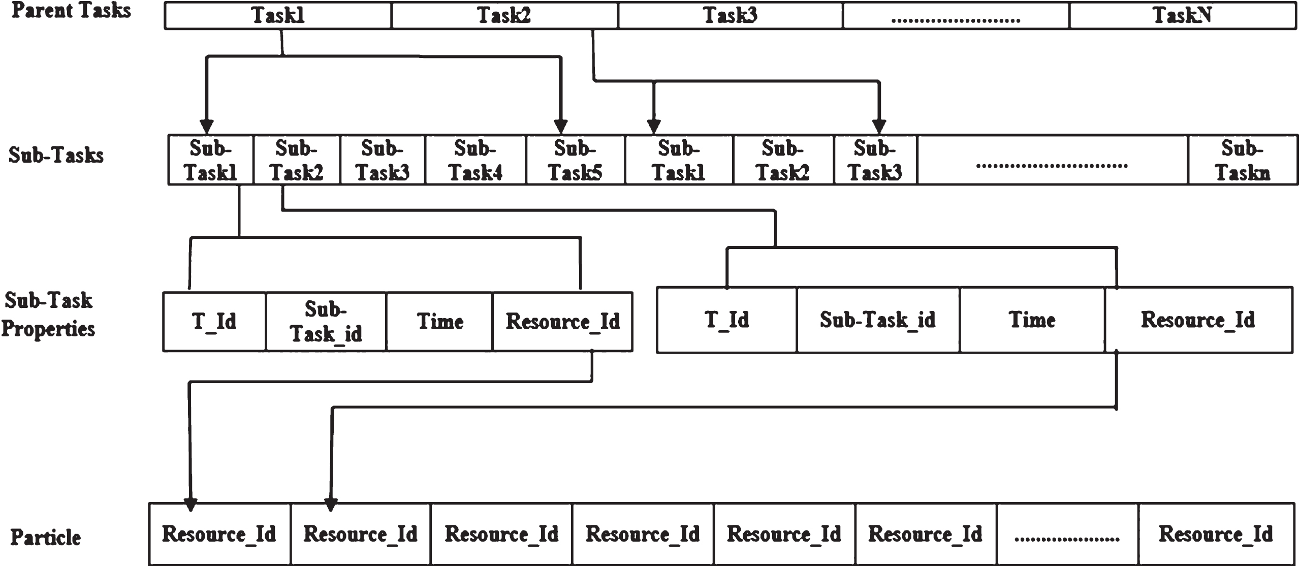
Particle Representation.

Fig. 2 shows that all N parent tasks (Task₁, Task₂, Task₃,..., Task_N) are divided randomly from 2 to 6 smaller subtask. In the above figure, Task₁ has 5 as a random number of subtasks, so, it is divided into 5 subtasks while Task₂ has only 3, so it is divided into 3 subtasks and so on. All subtasks are assigned to m resources randomly. Every subtask has four attributes: parent-task identification (T _ Id), subtask identification (Sub _ Task _ Id), completion time (Time) and the resource identification assigned to this subtask (Resource _ Id). In addition, the length of the particle is equal to the number of all subtasks. The components of the particle are all Resource _ Id assigned to the subtasks which are random numbers from 1 to 10 (For example: 1, 2, 3, 2, 4, 7, 4, 9, 10,...). Thus, our proposed MOPSO and MOPSO_IS algorithms are executed on this particle to produce the results.

4.4 The Proposed Algorithm

We consider a MO optimization problem. Then, the standard PSO needs to be modified for solving this problem. The MOPSO was presented in [33]. The MOPSO seeks to find a set of solutions called the Pareto set. In the beginning, the initial swarm is randomly generated. Then, a set of Gbest is initialized by using non-dominated particles from the swarm. The set of Gbest is stored in an external archive. In each iteration, a Gbest is selected, and the positions of the particles are updated. The turbulence operators are applied in MOPSO after updating the position. The set of Gbest is updated after all the processes of all the particles have finished. The main steps of the proposed MOPSO_IS algorithm is described as in Algorithm 1.

Algorithm 1: Main steps of MOPSO_IS algorithm
Input: A system state history and configuration
Output: Optimal fitness and results
for each particledo
random position and velocity.
evaluate fitness.
Pbest ← 0 position.
end for
update Gbest using IS strategy.
Whileterminationcriterion is fasle do
for each particle
update velocity and position.
apply Mutation.
evaluate fitness.
update Pbest position.
end for
update Gbest using IS strategy.
end while

The MOPSO algorithm is proposed to obtain the optimal solution for the cloud task scheduling problem. The first step is a list of tasks requests including attributes, quantity, and cost received. Then these tasks are divided into subtasks. These tasks with their attributes are distributed on the n swarm size. Where swarm size is the particles constituted a swarm, n is the number of tasks and m is the number of resources in the cloud environment. Every particle has a position and a velocity. The velocity was initialized as zero V_i = 0 and initialize the personal best of each particle Pbest_i = X_i and Gbest = Best particle is found in X_i. Then, the non-dominated particle vectors found in X_i are stored into the external archive. Next, it selects the Gbest guide for X_i from the external archive using IS and its position to Gbest and updates the new velocity and position by equations 8 and 9. Later, it performs mutation on X_i. Finally, the end of this loop evaluates X_i.

The next step is inserting all new non-dominated solution in X_i into the external archive if they are not dominated by any of the stored solutions. All dominated solutions in the archive by the new solution are removed from the archive. If the archive is full, the solution to be replaced is determined. Hence, the personal best solution of each particle in X_i is updated. If the current Pbest_i dominates the position in memory, the particles position is updated using Pbest_i = X_i. These steps should be repeated until Maximum iteration is reached. The flowchart of MOPSO_IS is shown in Fig. 3.

Fig.3

The MOPSO_IS Flowchart

4.5 External Archive

As mentioned above, the external archive for the non-dominated solutions found so far is stored. One of these solutions is used as a leader to update the positions of the particle. Also, it is used as the final optimal solution of the algorithm. Adding to the external archive in the beginning of the initialization by non-dominance solutions appears after evaluating the particles by the three objective functions. Then, after updating the position and evaluating the new particle, the external archive needs to be updated and new non-dominance solutions need to be added. Meanwhile, the deletion method is used for deleting redundant and non-dominant solutions when the external archive becomes full [31].

4.6 Leader Selecting Methods

The choice of the leader represents a very important part of the algorithm, so there are many methods or strategies used to select the leader. These methods like the density method, crowding distance [32] and Pareto-based approaches and combined method using weighting and other proposed new strategies. In this study, a new strategy known as IS is integrated and its results are compared with another method known as the weighting method.

4.6.1 Importance Strategy (IS)

A very closed idea of IS is used with MOGA in [11] for choosing the best chromosome in every population. Here, it is formulated to be used for selecting a Gbest leader. It produced better results compared to the weighted objective approach. This strategy uses three objective functions: total task time (Ftotal), average completion time (Favg) and load balancing (Fstd) with each having different importance. Assuming that the importance of the three objectives is Ftotal > Favg > Fstd. The pseudo-code of selecting a leader is shown as Algorithm 2.

Algorithm 2: IS Strategy for Selecting Gbest Leader
Input:Archive list (list of Gbest leaders)
Output: A selected best Gbest leader (LeaderId)
LeaderId ← 0
Fori ← 1 to ArchiveSize - 1 do
T_i=Archive . Ftotal (i)
T_L=Archive . Ftotal (LeaderId)
S_i=Archive . Fstd (i)
S_L=Archive . Fstd (LeaderId)
A_i=Archive . Favg (i)
A_L=Archive . Favg (LeaderId)
ifT_i > T_Lthen
LeaderId ← i;
else ifT_i = T_LandS_i > S_Lthen
LeaderId ← i;
else ifT_i = T_LandS_i = S_LandA_i > A_L
then
LeaderId←i;
end if
end for

For more details, the above algorithm is started with leaderId = 0 and the loop started from 1 to ArchiveSize - 1 to look for the particle that had the best Gbest among the list elements. The IS strategy works based on the importance of the three objectives: Ftotal > Favg > Fstd. That means, the Ftotal is the most important objective then Favg then Fstd. Thus, if the Fstd of the particle of index i is higher than it in the particle of index 0, then the LeaderId will be equal to index i. Otherwise, if both Fstd are equals and at the same time the second important objective Favg of index i is higher than it in the particle of index 0, then, the LeaderId will be equal to index i. Finally, if the two mentioned objectives are equals with the previous ones, respectively and at the same time the third important objective Fstd of the particle of index i is higher than it in particle of index 0, then, the LeaderId will be equal to index i and so on until i is reached to ArchiveSize - 1. The IS strategy obtains the best particle Gbest leader.

4.6.2 Weighting Method

Particles are considered as a vector of positions $\vec{X_{i}} = (X_{1}, X_{2}, . . ., X_{n})$ . In this method, specific weights were used for each of the three objective functions equal to -0.5. Thus, we assumed that the weighting is calculated using the following equation:

$QoS (\vec{X_{i}}) = \sum_{j = 1}^{q} w_{j} F_{j} (\vec{X_{i}})$

Where F is the number of objective functions and w is the weights of the three objectives. Before selecting a leader, the external archive must be sorted depending on QoS. The top one in the archive is selected as a leader.

4.7 Update Personal Best

Each particle has its own Pbest which is represented as an individual experience of it. The Pbest of each particle is updated based on dominance relations. It is measured in terms of a scalar value analogous to the fitness adopted in evolutionary algorithms. That means, the current solution is compared with the Pbest solution. If the current solution dominates the Pbest, Pbest will be replaced by the current solution.

4.8 Mutation Operation

The use of a mutation operator is very important in order to escape from local optima and to improve the exploratory capabilities of PSO. When a solution is chosen to be mutated each component is then mutated (randomly changed) or not with a certain probability. Actually, different mutation operators have been proposed that mutate components of either the position or the velocity of a particle. The choosing of a good mutation operator is a difficult task that has a significant impact on performance. Several proposed approaches use different mutation operators. The use of mutation operators in PSO is not new. It was proposed also to be used in [30 , 34]. The pseudo-code of a mutation operation is shown in Algorithm 3.

Algorithm 3: Mutation Operation Algorithm
Input: A particle i
Output: A mutated particle i
Mu ← 0.2;
randNum← RandomNumber;
ifrandNum < Muthen
NewSol = Mutate (Swarm [i] . Pos, Mu,L_low,L_high);
Swarm . evaluate (NewSol);
end if
if Dominat (NewSol . Cost, Swarm [i] . Cost)
then
Swarm [i] . Position ← NewSol _ pos;
Swarm [i] . Cost ← NewSol . Cost;
else ifDominat (Swarm [i] . Cost, NewSol . Cost)
then
do_Nothing
else if (randNum < 0.5) then
Swarm [i] . Position ← NewSol . Position;
Swarm [i] . Cost ← NewSol . Cost;
end if

More details of Algorithm 3: First of all, the Mu operator is fixed at 0.2. Then a random number randNum is generated. If this number is lower than Mu then the current particle is mutated as a new solution. Next, the mutated particle is evaluated based on the three objective functions. After that, we have to know if this new particle (new solution) dominates the old particle (old solution) by calling the Dominat () function. If the new solution dominates the old solution, then the old particle position of the old solution is replaced by the position of the new solution and the old cost is replaced with the new cost too. Otherwise, if the old particle dominates the new particle, nothing happened and the particle was not mutated. Lastly, the algorithm gives more chances for doing the mutation operation if the randNum is lower than 0.5.

5 Performance Evaluation

In this section, we present the experiments conducted to evaluate the performance of our algorithms.

5.1 Experiment Design

We carry out many experiments to measure the performance of the proposed algorithms against other algorithms. All algorithms were implemented in Java Eclipse IDE and the simulation was run on CPU core i5, memory 6 Gigabyte.

The proposed MOPSO algorithm with the two leader selection strategies was configured at the beginning of the experiment. In MOGA, the probability of the mutation (pm) will be 0.1 and the probability of the crossover (pc) is 0.8. In MOPSO, the acceleration coefficients parameters c₁ and c₂ are equal to 1.5, MaxVel is 4.5, Inertia weight (w) is 0.1, Mutation rate (Mu) is 0.2. Table 6 and Table 7 are summarized in the system configurations. Our experiment runs for 300 iterations for each algorithm to produce the average results. The results are also taken for different iterations from 0 to 300.

Table 3
MOPSO and MOPSO_IS Algorithms Parameters

Parameter Value(s) Parameter Value(s)

Swarm Size 100 c₁,c₂ 1.5

N 300 r₁, r₂ between [0,1]

m 10 Mu 0.2

ArchiveSize 20 w 0.2

Max. Iteration 300 MaxVel 4.5

Parameter	Value(s)	Parameter	Value(s)
Swarm Size	100	c₁,c₂	1.5
N	300	r₁, r₂	between [0,1]
m	10	Mu	0.2
ArchiveSize	20	w	0.2
Max. Iteration	300	MaxVel	4.5

Table 4

MOGA Algorithm Parameters

Parameter	Value(s)	Parameter	Value(s)
Population Size	100	N	300
m	10	Max Iteration	300
pm	0.1	pc	0.8

5.2 Results and Analysis

For each objective, two experiments were carried out in this research. The setting of the first experiment is discussed in Tables 3 and 4. The second experiment was repeated with a different number of tasks (300, 400, and 500) which are noted as Small, Middle and Large, respectively. The performance evaluation based on the measurements are elaborated on in the cost model. The experiments were conducted for the proposed MOPSO_IS, MOPSO and MOGA algorithms for total task time, the average task time and load balancing.

5.2.1 Total Task Time

The result of the first experiment is illustrated in Fig. 4. It shows the comparison of the total task time for the three algorithms. It is clearly shown that MOPSO_IS decreases the total task time. For the small iterations until 30, MOPSO_IS result is closed to the other two algorithms. The performance of MOPSO and MOPSO_IS algorithm is clearly improved at iteration 50. MOPSO_IS is significantly better than the two algorithms after iteration 140.

Fig.4

Total Task Time of the Three Algorithms.

Moreover, the result of the second experiment shows that, in the Small tasks, MOPSO_IS is 1% better than MOPSO and better than MOGA by 6%. For the Middle tasks, MOPSO_IS is 2% better than MOPSO and better than MOGA by 4%. In the Large tasks, MOPSO_IS is 4% better than MOPSO and better than MOGA by 10% times. Thus, the proposed algorithm has the lowest total task time in any load of tasks as clearly shown in Fig. 5.

Fig.5

Total Task Time of the Three Algorithms.

5.2.2 Average Task Time

Fig. 6 shows the average task time of the proposed MOPSO_IS, original MOPSO and MOGA algorithms. It is clear that the average task time of the proposed MOPSO_IS algorithm is lower than the other two algorithms. In the earlier iterations from 0 to 20, MOPSO_IS is not different from the other two algorithms. The improvement of proposed MOPSO and MOPSO_IS is clearly shown after iteration 40. MOPSO_IS is clearly better than the two algorithms after iteration 120.

Fig.6

Average Task Time of the Three Algorithms.

Furthermore, in the Small tasks, MOPSO_IS is 1% better than MOPSO and better than MOGA by 2%. For the Middle tasks, MOPSO_IS is 6% better than MOPSO and better than MOGA by 7%. In the Large tasks, the MOPSO_IS is 4% better than MOPSO and better than MOGA by 9%. It is clear that the proposed MOPSO_IS algorithm has the lowest average task time in any load of tasks as shown in Fig. 7.

Fig.7

Average Task Time of the Three Algorithms.

5.2.3 Load Balancing

It can be argued here that the load balancing of the proposed MOPSO_IS algorithm is better than the other two algorithms. In the earlier iterations from 0 to 20 the MOPSO_IS is not different from the other two algorithms. The differences are clearly shown at iteration 40. In an average, load balancing in MOPSO_IS is 70% better than MOGA. MOPSO is slightly better than MOPSO_IS for a small number of iteration. After iteration 240, MOPSO_IS is 16% better than MOPSO as plotted in Fig. 8.

Fig.8

Load Balancing of the Three Algorithms.

Moreover, Fig. 9 shows the average task time of the three algorithms for different task size. In all tasks size, MOPSO_IS is 20% better than MOPSO and better than MOGA by 80% in an average.

Fig.9

Load Balancing of the Three Algorithms.

Giving the MOPSO_IS algorithm a better load balancing, explained why it was given better performance in terms of total task time and average task time than others.

It is clear that the greatest opportunity in the improvement of the total tasks time, despite the early iterations of the emergence of a relatively lower reduction of the load balancing and average task time was more than what was in the last iterations. MOPSO algorithm is more robust than the MOGA algorithm because during the exploration of the search space, all particles guided by the best global position move towards the minimum value of the objectives. On the other hand, it was noted that MOPSO was more stable in orientation to the optimal solution than MOGA. The difference between the rise and fall in the MOGA compared to MOPSO, which was moving each time towards a better solution based on previous experience available through Pbest and Gbest. In Figs. 4-9, it is shown that the strategy of importance that integrated with MOPSO_IS gives better results than the previous methods but gives the same approximation to the optimal solution in 140 iterations as in the MOPSO algorithm. Table 5 shows the comparison of the mean value of the three algorithms for 50 sample data. This table clearly shows the performance of MOPSO_IS for the three objective functions.

Table 5

Performance Comparison

Algorithm	totTime	avgTime	stdD	Convergance
MOPSO_IS	1415.58	1408.67	4.7097	140
MOPSO	1428.22	1415.49	7.8578	140
MOGA	1503.12	1442.35	52.3328	240

5.2.4 Execution time

PSO algorithm was found to be the best performer among other algorithms in terms of execution time [35]. This is due to the fact that MOPSO_IS had fewer steps. Another reason was the integration of MOPSO with the mutation operator. The execution time was calculated for all tasks in each of the 10 resources. It was observed that the execution time of the 10 resources by the proposed algorithm was converging faster than the MOPSO and MOGA as shown in Fig. 10.

Fig.10

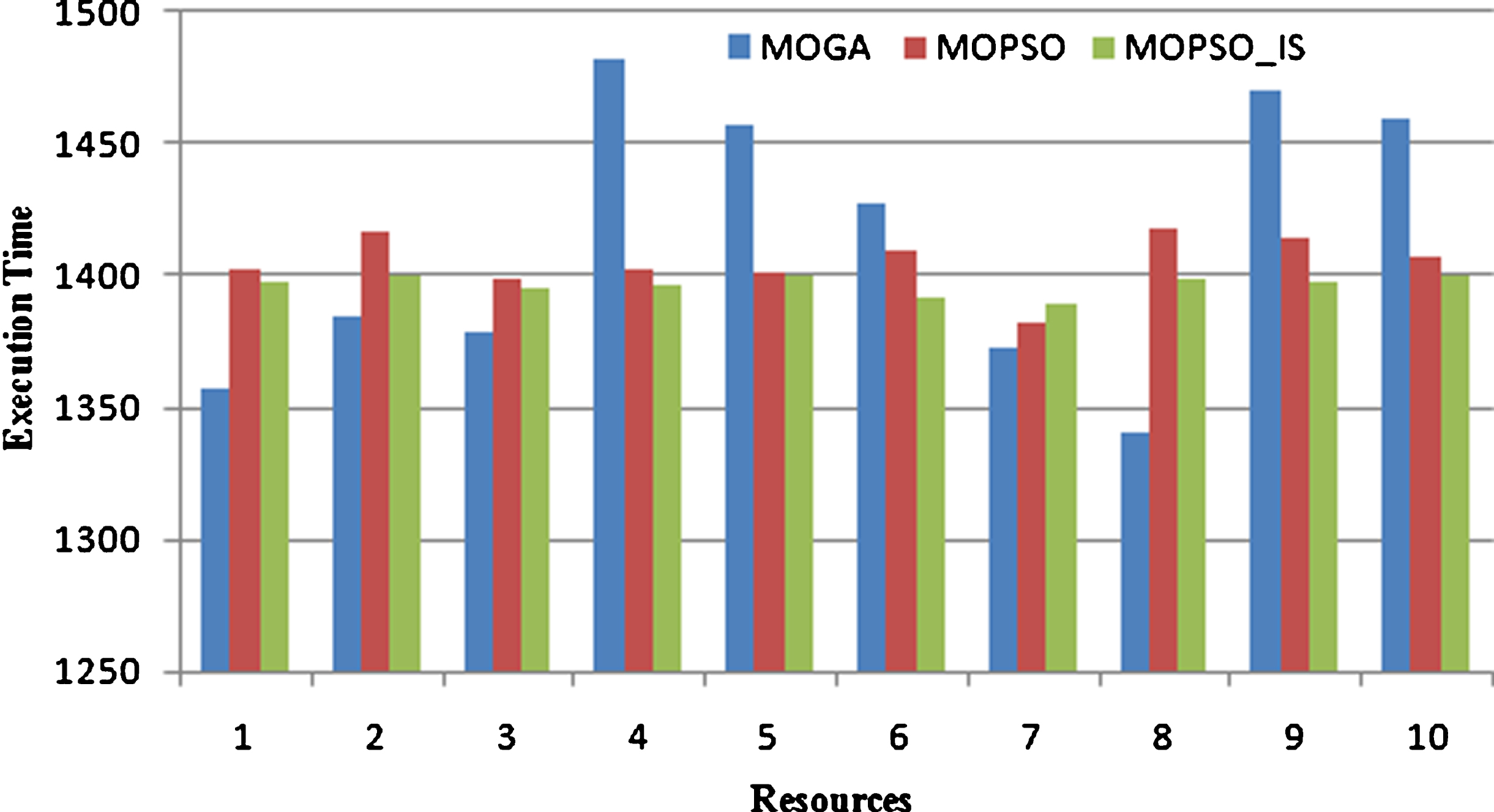
Execution Time of the Three Algorithms.

Fig.11

Execution Time of the Three Algorithms.

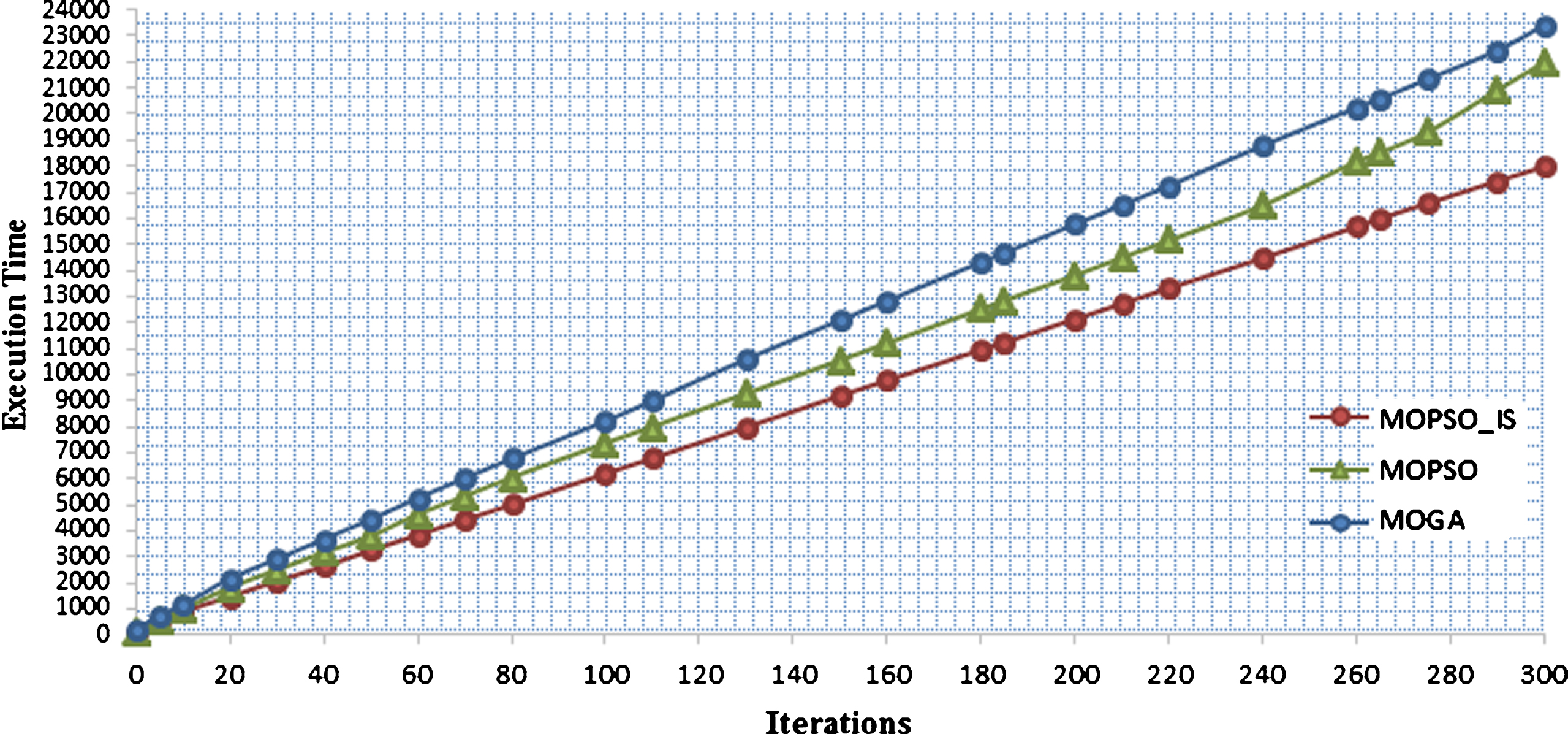
Thus, MOPSO_IS algorithm does not only improve the results but it also reduces the execution time of the scheduling algorithm. For 300 tasks, MOPSO_IS is 17% faster than MOPSO and faster than MOGA by 23%. The execution time of the three algorithms is clearly shown in Fig. 11.

6 Conclusion

This paper presented the integrated MOPSO_IS algorithm for cloud task scheduling. An IS strategy was integrated with the MOPSO algorithm to maintain the diversity of non-dominated solutions in the external archive. Thus, using the IS provided a well-distributed setting of non-dominated solutions and gave better performance. Although MOPSO_IS minimizes both total task time and average task time, it is also better based on load balancing. Moreover, the integration with the mutation operator was converged the MOPSO_IS very fast and reduced the algorithm execution time.

For future works, it might be of interest to study the performance under the following cases: extending the research by taking into account other parameters for more complex system and taking into account priority between the tasks in scheduling processes and using another selecting leader strategy.

References

Zhan

Z.-H.

, Liu

X.-F.

, Gong

Y.-J.

, Zhang

etal., Cloud computing resource scheduling and a survey of its evolutionary approaches, ACM Computing Surveys 47(4) (2015), 1–33.

Abdullah

, Lu

, Wieder

and Yahyapour

, A heuristic-based approach for dynamic VMs consolidation in cloud data centers, Arabian Journal for Science and Engineering 42(8) (2017), 3535–3549.

Buyya

, Broberg

and Goscinski

A.M.

, Cloud computing: Principles and paradigms, John Wiley & Sons, 87, 2010.

Buyya

, Yeo

C.S.

, Venugopal

and Brandic

J.I.

, Cloud computing and emerging it platforms: Vision, hype, and reality for delivering computing as the 5th utility, Future Generation Computer Systems 25(6) (2009), 599–616.

Lin

Y.-T.

, Wen

M.-L.

, Jou

and Wu

D.-W.

, A cloud-based learning environment for developing student reflection abilities, Computers in Human Behavior 32 (2014), 244–252.

Barley

, Cloud computing’s effect on enterprises-in terms of cost and security, Lund University, 2011.

Zahra

, Mohammad

, Bahman

and Ajith

, Using imperialist competition algorithm for independent task scheduling in grid computing, Journal of Intelligent & Fuzzy Systems 27(1) (2014), 187–199.

Pacini

, Mateos

and Garino

C.G.

, Distributed job scheduling based on Swarm Intelligence: A survey, Computers & Electrical Engineering 40(1) (2014), 252–269.

Keshanchi

and Navimipour

N.J.

, Priority-based task scheduling in the cloud systems using a memetic algorithm, Journal of Circuits, Systems and Computers 25(10) (2016), 1–33.

10.

Ramezani

, Lu

and Hussain

, Task scheduling optimization in cloud computing applying multi-objective particle swarm optimization, Proceeding of the International Conference on Service-Oriented Computing, Springer, 2013, pp. 237–251.

11.

, Xu

and Zhao

, Task scheduling based on multiobjective genetic algorithm in cloud computing, Journal of Information & Computational Science 12(4) (2015), 1429–1438.

12.

Feng

, Wang

, Zhang

and Li

, Multi-objective particle swarm optimization for resource allocation in cloud computing, Proceedings of the IEEE 2nd International Conference on Cloud Computing and Intelligent Systems 3 (2012), 1161–1165.

13.

Chen

and Guo

, Real-time task scheduling algorithm for cloud computing based on particle swarm optimization, Proceedings of the International Conference on Cloud Computing and Big Data in Asia, Springer, 2015, pp. 141–152.

14.

Awad

, El-Hefnawy

and Abdel

, kader, Enhanced particle swarm optimization for task scheduling in cloud computing environments, Procedia Computer Science 65 (2015), 920–929.

15.

Boloor

, Chirkova

, Salo

and Viniotis

, Heuristic-based request scheduling subject to a percentile response time SLA in a distributed cloud, Proceedings of the IEEE Global Telecommunications Conference (GLOBECOM 2010) 2010, pp.1–6.

16.

J.W.

and Yuan

Y.S.

, Research of cloud computing task scheduling algorithm based on improved genetic algorithm, Applied Mechanics and Materials 347 (2013), 2426–2429.

17.

Kennedy

and Eberhart

, Particle swarm optimization, Proceedings of the IEEE International Conference on Neural Networks (ICNN 95) 4 (1995), 1942–1948.

18.

Guo

, Zhao

, Shen

and Jiang

, Task scheduling optimization in cloud computing based on heuristic algorithm, Journal of Networks 7(3) (2012), 547–553.

19.

Pandey

, Wu

, Guru

S.M.

and Buyya

, A particle swarm optimization-based heuristic for scheduling workflow applications in cloud computing environments, Proceedings of the 24th IEEE International Conference on Advanced Information Networking and Applications (AINA), 2010, pp. 400–407.

20.

Mezmaz

, Lee

Y.C.

, Melab

, Talbi

E.-G.

and Zomaya

A.Y.

, A bi-objective hybrid genetic algorithm to minimize energy consumption and makespan for precce-constrained applications using dynamic voltage scaling, Proceedings of the IEEE Congress on Evolutionary Computation (CEC), 2010, pp. 1–8 eden.

21.

Somasundaram

T.S.

and Govindarajan

, CLOUDRB: A framework for scheduling and anaging High Performance Computing (HPC) applications in science cloud, Future Generation Computer System 34 (2014), 47–65.

22.

Jena

, Multi objective task scheduling in cloud environment using nested PSO framework, Procedia Computer Science 57 (2015), 1219–1227.

23.

Lashkari

and Moattar

M.H.

, The improved k-means clustering algorithm using the proposed extended PSO algorithm, Proceedings of the International Congress on Technology, Communication and Knowledge (ICTCK), 2015, pp. 429–434.

24.

Gupta

, Gajera

, Jana

P.K.

et al., An effective multiobjective workow scheduling in cloud computing: A PSO based approach, Proceedings of the IEEE 9th International Conference on Contemporary Computing, 2016, pp. 1–6.

25.

Chiregi

and Navimipour

N.J.

, Trusted services identification in the cloud environment using the topological metrics, Karbala International Journal of Modern Science 2(3) (2016), 203–210.

26.

Keshanchi

, Souri

and Navimipour

N.J.

, An improved genetic algorithm for task scheduling in the cloud environments using the priority queues: Formal verification simulation, and statistical testing, Journal of Systems and Software 124 (2017), 1–21.

27.

Razaque

, Vennapusa

N.R.

, Soni

et al., Task scheduling in cloud computing, Proceedings of the Conference of Long Island Systems, Applications and Technology, 2016, pp. 1–5.

28.

Moore

and Chapman

, Department of Computer Science and Software Engineering, Auburn University, Application of particle swarm to multiobjective optimization 1999.

29.

Kumar

and Minz

, Multi-objective particle swarm optimization: An introduction, SmartCR 4(5) (2014), 335–353.

30.

Coello

C.A.C.

, Pulido

G.T.

and Lechuga

M.S.

, Handling multiple objectives with particle swarm optimization, IEEE Transactions on Evolutionary Computation 8(3) (2004), 256–279.

31.

Salazar

, Lechuga, Ph.D. thesis, University of Birmingham, Multi-objective optimisation using sharing in swarm optimisation algorithms 2009.

32.

Sheikholeslami

and Navimipour

N.J.

, Service allocation in the cloud environments using multi-objective particle swarm optimization algorithm based on crowding distance, Swarm and Evolutionary Computation 35 (2017), 53–64.

33.

Reyes-Sierra

and Coello

C.C.

, Multi-objective particle swarm optimizers: A survey of the state-of-the-art, Int J Comput Intell Res 2(3) (2006), 287–308.

34.

Rui

, Lixin

, Xin

and Ziyu

, A novel multiobjective PSO algorithm based on completionchecking, Journal of Intelligent & Fuzzy Systems 34(1) (2018), 321–333.

35.

NZanywayingoma

and Yang

, Effective task scheduling and dynamic resource optimization based on heuristic algorithms in cloud computing environment, KSII Transaction on Internet and Information Systems 11(12) (2017), 5780–5802.

Integrated MOPSO algorithms for task scheduling in cloud computing

Abstract

Keywords

1 Introduction

3 General Description of the Scheduling Problem

3.1 Problem Formulation

3.2 Notations and Definitions

4.1 PSO Manipulation

4.3 Encoding Particle and Initial Swarm Generating

4.6 Leader Selecting Methods

4.6.1 Importance Strategy (IS)

4.6.2 Weighting Method

4.7 Update Personal Best

4.8 Mutation Operation

5 Performance Evaluation

5.1 Experiment Design

Table 3 MOPSO and MOPSO_IS Algorithms Parameters Parameter Value(s) Parameter Value(s) Swarm Size 100 c1,c2 1.5 N 300 r1, r2 between [0,1] m 10 Mu 0.2 ArchiveSize 20 w 0.2 Max. Iteration 300 MaxVel 4.5

5.2.1 Total Task Time

References

Table 3
MOPSO and MOPSO_IS Algorithms Parameters

Parameter Value(s) Parameter Value(s)

Swarm Size 100 c₁,c₂ 1.5

N 300 r₁, r₂ between [0,1]

m 10 Mu 0.2

ArchiveSize 20 w 0.2

Max. Iteration 300 MaxVel 4.5