Fuzzy demographic analysis using fuzzy regression models based on fuzzy distance–A case on the impact of fuzzy demographic factors on monetary aggregates in Canada versus Japan

Abstract

The concern for the relationship between demographic changes and asset markets has increased from beginning of 2000. Many researchers analyze the relationship between demographic changes and asset prices through regression models. Most of these studies apply linguistic terms for each different phase of the life cycle (e.g. late working-aged, elderly, adult, and middle-aged) and then define a specific behaviour for each of these cohorts. Although these terms are vague, all the researchers define them as a crisp set with crisp partitions. Additionally, fuzzy regression methods have attracted growing interest from researchers in various scientific, engineering, and humanities area due to the ambiguity in real data. The motivation of this research is that it is rational to consider and apply fuzzy sets to interpret these linguistic terms instead of the crisp partitions. In this study, we propose and apply a new approach in order to calculate the fuzzy frequency for the linguistic term, which can be useful in any other demographic study. Moreover, new fuzzy regression models are developed. These regression models, that are able to consider both fuzzy and crisp regression coefficients are developed based on applying a fuzzy distance concept in which the distance between two triangular fuzzy numbers (TFNs) or between a TFN and a crisp number is a TFN. Multi-objective optimization helps us to find the results without any compromise. The models are solved using the mathematical programming solver LINGO-16 to derive the fuzzy regression coefficients. We apply these models in a numerical example also in a real case study (fuzzy input, crisp output) in which an investigation on the relationship between fuzzy demographic dynamics and monetary aggregates is made.

Keywords

Fuzzy sets fuzzy demographic changes fuzzy regression fuzzy distance Marshallian K

1 Introduction

Regression analysis is a widespread technique in various applications from engineering to humanities and medical sciences. Fuzzy regression methods can be applied to consider both crisp and fuzzy data, including an imprecise relationship among variables and/or measurements. According to Muzzioli, et al. [1], the aim of fuzzy regression is to incorporate all the vagueness embedded in the data, without losing the information that is inevitably overridden when the original data is arbitrarily modified or the lack of precision cancelled.

Due to ambiguity in real data, it was expected that fuzzy regression would be more prevalent in data analysis like other fuzzy techniques (e.g., Fuzzy Inference Systems, FIS) since the first approach was introduced by Tanaka, et al. [2]. However, a variety of fuzzy regression models have been proposed with different characteristics in different applications. In the common classification of fuzzy regression research, two basic approaches are the mainstream in fuzzy regression models [3], with a hybrid approach also being used.

Possibilistic regression, based on a linear programming approach in order to minimize the fuzziness in the model [2 , 4–7]

Fuzzy least squares regression, which uses least squares of errors as a fitting criterion [8 –12].

Hybrid methods, which use the possibilistic and/or the least squares approach in which other techniques might be considered along with them [13].

Other classifications could be useful due to the common characteristics of various FR methods. These have been developed in this decade, including the following papers:

Classification based on fuzziness in input and/or output, (i.e., CIFO: Crisp Input Fuzzy Output [6 , 15], FIFO: Fuzzy Input Fuzzy Output [16 –19], FICO: Fuzzy Input Crisp Output).

Classification based on whether fuzziness in the regression coefficients is allowed [6 , 18], or not [20].

Classification based on fuzzy distance or a crisp index as the proxy of the fuzzy distances between output and real data [21 –25].

Recently, the distance measures and uncertain information are considered by intuitionistic fuzzy sets. The main advantage of this fuzzy-sets approach is that it is able to consider complex attitudinal characters of the decision-maker by using order-inducing variables in the aggregation of the distance measures [26]. Other recent extensions of fuzzy sets have been developed to model imprecise/incomplete information or other ambiguous in decision-making problems could be applied in future research. (E.g. Type-2 linguistic [27], Pythagorean fuzzy set [28, 29], Attitudinal consensus [30], Hesitant fuzzy set [31] Intuitionistic fuzzy preference relations (IFPRs) and Interval-valued fuzzy preference relations (IVFPRs) [32].)

This research was conducted within a larger project analyzing the relationship between demographic factors and asset values, an area of research that has expanded greatly since 2000 involving researchers in economics, finance, actuarial science and related disciplines. Many researchers analyze the relationship between demographic changes and asset prices through regression models. Most of these studies apply linguistic terms for each different phase of the life cycle (e.g. late working-aged, elderly, adult, and middle-aged) and then define a specific behaviour for each of these cohorts. Although these terms are vague, all the researchers define them as a crisp set with crisp partitions. In subsection 5-1 we identify some of the different age definitions used in the literature.

The motivation of this research is that it is rational to consider and apply fuzzy sets to interpret these linguistic terms instead of the crisp partitions. In this study, we propose and apply a new approach in order to calculate the fuzzy frequency for the linguistic term, which can be useful in any other demographic study. Moreover, new fuzzy regression models are developed. These regression models, that are able to consider both fuzzy and crisp regression coefficients are developed based on applying a fuzzy distance concept in which the distance between two triangular fuzzy numbers (TFNs) or between a TFN and a crisp number is a TFN. Multi-objective optimization helps us to find the results without any compromise. The models are solved using the mathematical programming solver LINGO-16 to derive the fuzzy regression coefficients. We apply these models in a numerical example also in a real case study (fuzzy input, crisp output) in which an investigation on the relationship between fuzzy demographic dynamics and monetary aggregates is made.

This paper is structured as follows. In the next subsection, we discuss the problems with using crisp partitions and explain the two aims of this paper: first, we adopt a fuzzy distance for two TFNs as well as multi-objective mathematical programming approach in order to develop new fuzzy regression models in two different scenarios - A crisp-coefficient FR, and a Fuzzy-coefficients FR; second, we show a new aspect of FR models in order to be applied in demographic analysis. In Section 2, we introduce the concept of the fuzzy distance between two triangular fuzzy numbers, which is used in the subsequent analysis. In Section 3, the new Fuzzy Input- Fuzzy Output Linear Regression (FIFO-LR) models, which consider crisp and fuzzy regression coefficients based on the fuzzy distance in multi-objective optimization problems, are developed. An example and implication of the proposed models are also presented in this section. Section 4 deals with the new approach in order to calculate the fuzzy frequency for the linguistic term, which is applied in demographic studies as an independent variable. After that, in Section 5, a case study analyzing work by Nishimura & Takats [33] shows a practical application of our approach, in which we present an investigation on the relationship between fuzzy demographic dynamics and monetary aggregates in Canada versus Japan. The paper finishes with conclusions gathered in Section 6.

1.1 Discussion regarding the problems of existing approaches

Consistency between the ambiguity of input and the ambiguity of output in a regression model is a critical issue. Most of the fuzzy regression techniques develop a model with a higher degree of ambiguity in order to fit its output to the actual output. This phenomenon is due to using a crisp measure as a proxy of distance in the fuzzy environment. However, the distance between two TFNs or between a TFN and a crisp number is a triangular fuzzy number [34 –36].

Let $\tilde{N} 1$ and $\tilde{N} 2$ be two triangular fuzzy numbers. By definition, triangular fuzzy number $\tilde{D} = (d_{l}, d_{m}, d_{u})$ is a fuzzy distance between $\tilde{N} 1$ and $\tilde{N} 2$ , where d_l, d_m and d_u are respectively the left point as the minimum distance, the centre point, and the right point as the maximum distance for the two fuzzy numbers $\tilde{N} 1$ and $\tilde{N} 2$ .

In all of the fuzzy distance definitions, d_u will increase with increasing ambiguity of $\tilde{N} 1$ or $\tilde{N} 2$ [34 –36]. Using a wider range of the regression coefficients in fuzzy regression models makes a better fit compared to the crisp distance case. However, it is not good in actual fuzzy calculations because an increase in d_u due to using the wider range of coefficients makes a worse fit.

As the first aim of this paper, we adopt a fuzzy distance for two TFNs as well as multi-objective mathematical programming approach in order to develop new fuzzy regression models in two different scenarios - A crisp-coefficient FR, and a Fuzzy-coefficients FR. We also show that these models are able to cover both prevalent crisp least-squares regression and possibilistic FR.

For crisp data, FR models are particularly useful when an ordinary regression model is not appropriate because it is impossible to verify distributional assumptions or derive a valid statistical relationship. However, as the second aim of this paper, in our case study, we show a new aspect of FR models in order to be applied in demographic analysis. Most of economic theories such as the life-cycle theory [37] use linguistic terms for demographic variables (e.g., population of young people, working-age people). In this paper, we introduce a fuzzy approach to quantify the frequency of these linguistic terms - as fuzzy demographic factors - in order to be applicable in the economic empirical tests. In the case study, this approach, along with the proposed fuzzy regression models are applied to investigate the demographic impact (as a fuzzy independent variable) on the monetary aggregates of Canada and Japan (as the response variable).

2 The distance for two triangular fuzzy numbers (TFNs)

The distances for two fuzzy numbers can be categorized in two main clusters:

The crisp distances: These types of distances explain the crisp values as a proxy of the distance between two fuzzy numbers. They were introduced earlier and have been used in clustering, ranking fuzzy numbers, and regression analysis.

The fuzzy distances: These distances introduce a fuzzy distance for normal fuzzy numbers. Voxman [34] introduced a fuzzy distance for the first time. He also stated how it is possible for the distance between two fuzzy numbers to be a crisp number.

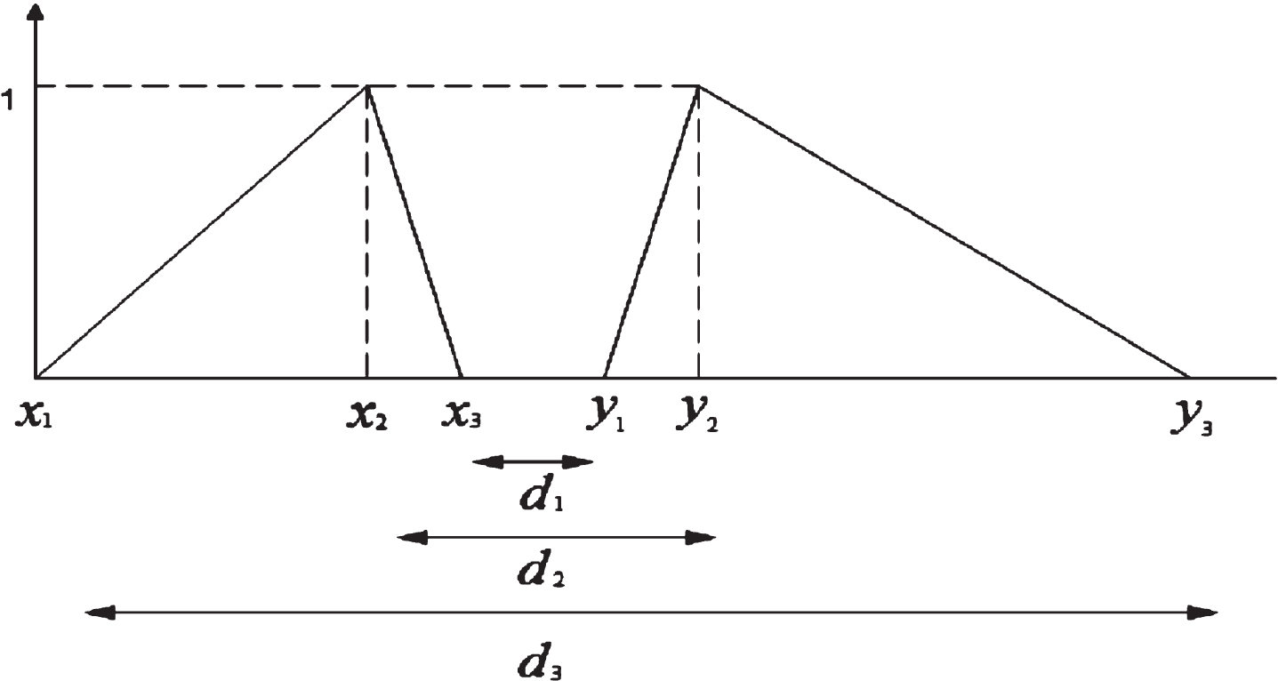
Chakraborty & Chakraborty [35] proposed another fuzzy distance in which the general fuzzy number was calculated by LR- Type fuzzy number. Sadi-Nezhad, et al. [36] introduced another fuzzy distance which is applied in fuzzy clustering [38, 39]. Based on their definition, we apply the fuzzy distance for two triangular fuzzy numbers as follows:

Definition 1. Let $\tilde{x} = (x_{1}, x_{2}, x_{3})$ and $\tilde{y} = (y_{1}, y_{2}, y_{3})$ be two triangular fuzzy numbers (TFNs). Triangular fuzzy number D_xy = (d₁, d₂, d₃), is defined as a fuzzy distance between $\tilde{x}$ and $\tilde{y}$ , where d₁, d₂ and d₃ are respectively the left point, center and right points subject to: $d_{1} = {\begin{matrix} max {x_{1} - y_{3}, 0} x_{2} ⩾ y_{2} \\ max {y_{1} - x_{3}, 0} x_{2} ⩽ y_{2} \end{matrix}$ $d_{2} = | x_{2} - y_{2} |$ $d_{3} = {max (y_{3} - x_{1}, x_{3} - y_{1})}$

Figure 1 shows this fuzzy distance.

Fig.1 3 Proposed fuzzy regression models based on the fuzzy distance

3.1 Scenario 1: Fuzzy input- Fuzzy output linear regression (FIFO-LR) with crisp coefficients based on fuzzy distance

A linear combination of the explanatory variables is assumed in FLR analysis. A sample of n observations, ${({\tilde{p}}_{i}, {\tilde{X}}_{i}), i = 1 to n}$ , is the basis of this relationship. Where for observation i, ${\tilde{p}}_{i}$ is the ith observed fuzzy output in form of a Triangular Fuzzy Number (TFN), , and $\tilde{X} = ({\tilde{x}}_{i 0}, {\tilde{x}}_{i 1}, \dots, {\tilde{x}}_{ij}, \dots, {\tilde{x}}_{ik})$ is the ith observed fuzzy input vector in form of a Triangular Fuzzy Number (TFN). ${\tilde{x}}_{ij}$ is the real value for the jth variable in the ith case of the sample and ${\tilde{x}}_{i 0} = 1$ for all i = 1 to n.

The fuzzy linear function to be estimated is as follows: $\tilde{y_{l}} = \sum_{j = 0}^{k} B_{j} {\tilde{x}}_{ij}$ (1)

Where $\tilde{y_{l}}$ is the fuzzy estimation of y_i in terms of TFN, and B_j, j = 0, 1, ... , k, are crisp coefficients, which can be determined by solving a FLR model. Each triangular fuzzy number ${\tilde{x}}_{ij}$ is a triplet ${\tilde{x}}_{ij} = ({x_{ij}}^{L}, {x_{ij}}^{M}, {x_{ij}}^{U})$ for i = 0, ... , n and j = 0, ... , k, where x_ij^L is the lower bound, x_ij^M is the central value and x_ij^U is the upper bound. The fuzzy regression due to its fuzzy input depends on the sign of regression coefficients. The fuzzy regression is as follows:

$\tilde{y_{l}} = (f_{L} ({\tilde{X}}_{i}), f_{M} ({\tilde{X}}_{i}), f_{U} ({\tilde{X}}_{i}))$ , where $f_{L} ({\tilde{X}}_{i})$ is the lower bound, $f_{M} ({\tilde{X}}_{i})$ the central value, and $f_{U} ({\tilde{X}}_{i})$ the upper bound of the $\tilde{y_{l}}$ as a TFN. From fuzzy arithmetic, the model as a triplet follows that: $f_{L} ({\tilde{X}}_{i}) = \sum_{0 \underset{B_{j} ⩾ 0}{⩽ j ⩽ k}} B_{j} x_{ij}^{L} + \sum_{\underset{B_{j} ⩽ 0}{0 ⩽ j ⩽ k}} B_{j} x_{ij}^{U}$ (2) $f_{M} ({\tilde{X}}_{i}) = \sum_{j = 0}^{k} B_{j} {x_{ij}}^{M}$ (3) $f_{U} ({\tilde{X}}_{i}) = \sum_{\underset{{\overset{`}{B}}_{j} ⩾ 0}{0 ⩽ j ⩽ k}} B_{j} x_{ij}^{U} + \sum_{\underset{{\overset{`}{B}}_{j} ⩽ 0}{0 ⩽ j ⩽ k}} B_{j} x_{ij}^{L}$ (4)

Where ${\overset{`}{B}}_{j}$ is the regression coefficient for j_th variable when using only $x_{ij}^{M}$ in a crisp linear regression at the prerequisite stage. (Equations (2) and (4) use only the sign of ${\overset{`}{B}}_{j}$ .

We define triangular fuzzy number ${\tilde{D}}_{i}$ as a fuzzy distance between fuzzy estimation $\tilde{y_{l}}$ and the fuzzy value for the ith case of the sample as follows: ${\tilde{D}}_{i} = (d_{li}, d_{mi}, d_{ui})$ (5)

Where d_li, d_mi and d_ui are respectively the left point, centre and right point. According to the definition1, d_li, d_mi and d_ui are as follows: $d_{li} = {\begin{matrix} max {p l_{i} - f_{U} ({\tilde{X}}_{i}), 0} p m_{i} ⩾ f_{M} ({\tilde{X}}_{i}) \\ max {f_{L} ({\tilde{X}}_{i}) - p u_{i}, 0} p m_{i} ⩾ f_{M} ({\tilde{X}}_{i}) \end{matrix}$ (6) $d_{mi} = | p m_{i} - f_{M} ({\tilde{X}}_{i}) |$ (7) $d_{ui} = {max (f_{U} ({\tilde{X}}_{i}) - p l_{i}, p u_{i} - f_{L} ({\tilde{X}}_{i}))}$ (8)

Model 1: A least squares fuzzy regression model with crisp regression coefficients

A quadratic programming with linear constraints model based on the least squares fuzzy regression approach leads to $Min Z = \sum_{i = 1}^{n} {\tilde{D}}_{i}^{2}$ as the fuzzy objective function.

This fuzzy objective function is converted to a multi-objective as follows Chen & Hwang [40]: ${\begin{matrix} Min Z_{1} = \sum_{i = 1}^{n} {d_{li}}^{2} \\ Min Z_{2} = \sum_{i = 1}^{n} {d_{mi}}^{2} \\ Min Z_{3} = \sum_{i = 1}^{n} {d_{ui}}^{2} \end{matrix}$ (9)

The final solution of a rational decision maker (DM) is always Pareto optimal, thus we can restrict our consideration to Pareto optimal solutions techniques [41]. Multi-objective models with fuzzy coefficients are always an NP hard problem, and they are especially difficult for nonlinear programming [42] or fuzzy random variables [43, 44]. We suggest the global criterion method in order to consider all objectives as a single objective. However, interactive approaches such as trade-off based methods are more preferable if the DM is available and willing to be involved in the solution process and direct it according to her/his preferences [41]. Model 1, as a crisp quadratic programming with linear constraints model, considers all the aspects.

Model (1) $Min Z_{T} = \sum (\frac{Z_{i} - Z_{i}^{*}}{Z_{i}^{*}})$ $St : p m_{i} - f_{M} ({\tilde{X}}_{i}) + L_{i} - U_{i} = 0$ $d_{mi} = Li + U_{i}$ $d_{li} + f_{U} ({\tilde{X}}_{i}) ⩾ p l_{i}$ $- d_{li} + f_{L} ({\tilde{X}}_{i}) ⩽ p u_{i}$ $d_{ui} ⩾ f_{U} ({\tilde{X}}_{i}) - p l_{i}$ $d_{ui} ⩾ p u_{i} - f_{L} ({\tilde{X}}_{i})$ $d_{ui}, d_{mi}, d_{li}, L_{i}, U_{i} \geq 0 and B_{j} isfreeinsign$

We define $Z_{i}^{*}$ from equation 9 as the optimal solution when Z_i is considered as the only single objective in the model. (However, Z₁ can be omitted because it is always dominated by Z₂ and Z₃.)

Model 2: A linear programming model with crisp regression coefficients

In order to develop a linear programming model, we define $\frac{d_{ui}}{| p u_{i} |}, \frac{d_{mi}}{| p m_{i} |}$ , and $\frac{d_{li}}{| p l_{i} |}$ as the relative maximum distance, relative centre distance, and relative minimum distance, respectively for ith case of the sample. As a result, the multi-objective changes as follows. $Min F_{1} = \sum_{i = 1}^{n} \frac{d_{li}}{| p l_{i} |}$ $Min F_{2} = \sum_{i = 1}^{n} \frac{d_{mi}}{| p m_{i} |}$ $Min F_{3} = \sum_{i = 1}^{n} \frac{d_{ui}}{| p u_{i} |}$

Model 2 is a linear programming model in which $F_{i}^{*}$ is the optimal solution of the model when F_i is considered as the only single objective.

Model (2) $Min Z_{w} = \sum (\frac{F_{i} - F_{i}^{*}}{F_{i}^{*}})$ $St : p m_{i} - f_{M} ({\tilde{X}}_{i}) + L_{i} - U_{i} = 0$ $d_{mi} = L_{i} + U_{i}$ $d_{li} + f_{U} ({\tilde{X}}_{i}) ⩾ p l_{i}$ $- d_{li} + f_{L} ({\tilde{X}}_{i}) ⩽ p u_{i}$ $d_{ui} ⩾ f_{U} ({\tilde{X}}_{i}) - p l_{i}$ $d_{ui} ⩾ p u_{i} - f_{L} ({\tilde{X}}_{i})$ $d_{ui}, d_{mi}, d_{li}, L_{i}, U_{i} \geq 0 and B_{j} is free \in sign$

3.2 Scenario 2: Fuzzy input- Fuzzy output linear regression (FICO-LR) with TFN coefficients

Similar to the scenario 1, a linear combination of the explanatory variables is assumed in the FLR analysis in this scenario. A sample of n observations, , is the base of this relationship. Where for observation i, ${\tilde{p}}_{i}$ is the ith observed fuzzy output in form of Triangular Fuzzy Number (TFN), ${\tilde{p}}_{i} = (p l_{i}, p m_{i}, p u_{i})$ , and ${\tilde{X}}_{i} = ({\tilde{x}}_{i 0}, {\tilde{x}}_{i 1}, \dots, {\tilde{x}}_{ij}, \dots, {\tilde{x}}_{ik})$ is the ith observed fuzzy input vector in form of Triangular Fuzzy Number (TFN). ${\tilde{x}}_{ij}$ is the real value for the jth variable in the ith case of the sample and ${\tilde{x}}_{i 0} = 1$ for all i = 1 to n.

The fuzzy linear function to be estimated is as follows: $\tilde{y_{l}} = \sum_{j = 1}^{k} {\tilde{B}}_{j} {\tilde{x}}_{ij}$ (10)

Where $\tilde{y_{l}}$ is the fuzzy estimation of y_i, and ${\tilde{B}}_{j}, j = 0, 1, \dots, k$ , are fuzzy coefficients in terms of TFNs, which can be determined by solving an FLR model. Each Triangular Fuzzy Number, ${\tilde{x}}_{ij}$ , is a triplet ${\tilde{x}}_{ij} = ({x_{ij}}^{L}, {x_{ij}}^{M}, {x_{ij}}^{U})$ i = 0, ... , n and j = 0, ... , k, where x_ij^L is the lower bound, x_ij^M is the central value and x_ij^U is the upper bound. Each triangular fuzzy number ${\tilde{B}}_{j}$ is a triplet ${\tilde{B}}_{j} = (B_{j}^{L}, B_{j}^{M}, B_{j}^{U})$ j = 0, ... , k, where $B_{j}^{L}$ is the lower bound, $B_{j}^{M}$ is the central value and $B_{j}^{U}$ is the upper bound. The fuzzy regression due to its fuzzy input depends on the sign of regression coefficients. The fuzzy regression is as follows:

$\tilde{y_{l}} = (g_{L} ({\tilde{X}}_{i}), g_{M} ({\tilde{X}}_{i}), g_{U} ({\tilde{X}}_{i}))$ , where $g_{L} ({\tilde{X}}_{i})$ is the lower bound, $g_{M} ({\tilde{X}}_{i})$ the central value, and $g_{U} ({\tilde{X}}_{i})$ the upper bound of the $\tilde{y_{l}}$ as a TFN. From fuzzy arithmetic, the model as a triplet follows: $\begin{matrix} \begin{matrix} g_{L} ({\tilde{X}}_{i}) = \\ \sum_{\begin{matrix} 0 ⩽ j ⩽ k \\ {\tilde{B}}_{j} ⩾ 0, x_{ij}^{L} ⩽ 0 \end{matrix}} B_{j}^{U} x_{ij}^{L} + \sum_{\begin{matrix} 0 ⩽ j ⩽ k \\ {\tilde{B}}_{j} ⩾ 0, x_{ij}^{L} ⩾ 0 \end{matrix}} B_{j}^{L} x_{ij}^{L} + \\ \sum_{\begin{matrix} 0 ⩽ j ⩽ k \\ {\tilde{B}}_{j} ⩽ 0, x_{ij}^{L} ⩽ 0 \end{matrix}} B_{j}^{U} x_{ij}^{U} + \sum_{\begin{matrix} 0 ⩽ j ⩽ k \\ {\tilde{B}}_{j} ⩽ 0, x_{ij}^{L} ⩾ 0 \end{matrix}} B_{j}^{U} x_{ij}^{L} \end{matrix} \end{matrix}$ $g_{M} ({\tilde{X}}_{i}) = \sum_{j = 0}^{k} B_{j}^{M} x_{ij}^{M}$ $\begin{matrix} \begin{matrix} g_{U} ({\tilde{X}}_{i}) = \\ \sum_{\begin{matrix} 0 ⩽ j ⩽ k \\ {\tilde{B}}_{j} ⩾ 0, x_{ij}^{U} ⩽ 0 \end{matrix}} B_{j}^{L} x_{ij}^{U} + \sum_{\begin{matrix} 0 ⩽ j ⩽ k \\ {\tilde{B}}_{j} ⩾ 0, x_{ij}^{U} ⩾ 0 \end{matrix}} B_{j}^{U} x_{ij}^{U} + \\ \sum_{\begin{matrix} 0 ⩽ j ⩽ k \\ {\tilde{B}}_{j} ⩽ 0, x_{ij}^{U} ⩽ 0 \end{matrix}} B_{j}^{L} x_{ij}^{L} + \sum_{\begin{matrix} 0 ⩽ j ⩽ k \\ {\tilde{B}}_{j} ⩽ 0, x_{ij}^{U} ⩾ 0 \end{matrix}} B_{j}^{U} x_{ij}^{L} \end{matrix} \end{matrix}$

Determining the regression coefficients is a two-stage process. The first stage determines the sign of the ${\ddot{B}}_{j}$ based on the minimization of least squares deviation approach in model 1 (FIFO-LR scenario 1).

Model 3: A least squares fuzzy regression model with TFN regression coefficients

Similar to the first model, we define $Z_{i}^{*}$ from equation 9 as the optimal solution when Z_i is considered as the only single objective in the model.

Model (3) $Min Z_{T} = \sum (\frac{Z_{i} - Z_{i}^{*}}{Z_{i}^{*}})$ $St : p m_{i} - g_{M} ({\tilde{X}}_{i}) + L_{i} - U_{i} = 0$ ${dmi}_{= Li + Ui}$ $d_{li} + g_{U} ({\tilde{X}}_{i}) ⩾ p l_{i}$ $- d_{li} + g_{L} ({\tilde{X}}_{i}) ⩽ p u_{i}$ $d_{ui} ⩾ g_{U} ({\tilde{X}}_{i}) - p l_{i}$ $d_{ui} ⩾ p u_{i} - g_{L} ({\tilde{X}}_{i})$ $\begin{matrix} d_{ui}, d_{mi}, d_{li}, L_{i}, U_{i} \\ ⩾ 0, and B_{j}^{L}, B_{j}^{M}, B_{j}^{U} are free in sign \end{matrix}$

As mentioned in the previous section, using a wide range of regression coefficients makes a worse fit. If one uses the same objective function of model 1 or 2 in model 3, the results of model 3 will not change materially in comparison to scenario 1.

3.3 Numerical example

To illustrate the suitability of the proposed fuzzy regression models for solving different types of fuzzy regression problems, we explore an example that is discussed in [22]. This example is a two dimensional linear regression with non-symmetric fuzzy input and fuzzy output. It is noteworthy that all of the previous researches has applied a crisp criterion in order to compare the goodness of fit for the total error between methods, and none of them applied a fuzzy distance. Our proposed models do not have any restrictions with respect to non-symmetrical data, negative input and output, negative intercept, and/or other regression coefficients.

This example includes fifteen observations, which are shown in Table 1.

Table 1
Fifteen fuzzy observations (input and output are TFNs)

Case i pl _i pm _i pu _i $x_{i 1}^{L}$ $x_{i 1}^{M}$ $x_{i 1}^{u}$ $x_{i 2}^{L}$ $x_{i 2}^{M}$ $x_{i 2}^{u}$

1 162.5 231.6 283 269 274 276 98 100 105

2 218 261 338 177 180 183 217 220 223

3 381.75 477 557.5 371 375 379 356 360 364

4 330.25 397 484.5 200 205 210 355 360 365

5 206.5 277.4 309 82 86 89 237 240 244

6 207.25 263 336.5 260 265 269 176 180 185

7 187.5 216.2 270 91 98 103 195 200 207

8 291 377 446 322 330 334 246 250 258

9 169.25 226 281.5 189 195 200 145 150 156

10 144.25 168.2 219.5 48 53 60 153 160 165

11 263.5 349 455 422 430 438 192 200 208

12 323 404.8 514 365 372 378 294 300 307

13 378 435.4 520 233 236 241 395 400 403

14 335.25 387.8 466.5 155 157 165 372 380 382

15 358.5 472 550 366 370 377 333 340 344

Case i	pl _i	pm _i	pu _i	$x_{i 1}^{L}$	$x_{i 1}^{M}$	$x_{i 1}^{u}$	$x_{i 2}^{L}$	$x_{i 2}^{M}$	$x_{i 2}^{u}$
1	162.5	231.6	283	269	274	276	98	100	105
2	218	261	338	177	180	183	217	220	223
3	381.75	477	557.5	371	375	379	356	360	364
4	330.25	397	484.5	200	205	210	355	360	365
5	206.5	277.4	309	82	86	89	237	240	244
6	207.25	263	336.5	260	265	269	176	180	185
7	187.5	216.2	270	91	98	103	195	200	207
8	291	377	446	322	330	334	246	250	258
9	169.25	226	281.5	189	195	200	145	150	156
10	144.25	168.2	219.5	48	53	60	153	160	165
11	263.5	349	455	422	430	438	192	200	208
12	323	404.8	514	365	372	378	294	300	307
13	378	435.4	520	233	236	241	395	400	403
14	335.25	387.8	466.5	155	157	165	372	380	382
15	358.5	472	550	366	370	377	333	340	344

Models 1, 2, and 3 are solved using the mathematical programming solver LINGO-16 to derive the regression coefficients. These three fuzzy regression models are as follows: ${\tilde{y}}_{Model 1} = 23.3024 + 0.4085042 {\tilde{X}}_{1} + 0.8142598 {\tilde{X}}_{2}$ ${\tilde{y}}_{Model 2} = 18.83518 + 0.4569758 {\tilde{X}}_{1} + 0.7821569 {\tilde{X}}_{2}$ $\begin{matrix} {\tilde{y}}_{Model 3} = (17.312, 21.255, 24.47) + \\ (0.378, 0.418, 0.428) {\tilde{X}}_{1} + (0.794, 0.809, \\ 0.835) {\tilde{X}}_{2} \end{matrix}$

Table 2 depicts the fuzzy distance between the real fuzzy observations and the fuzzy output for all the fifteenth cases. Figures 2–4 show the output of these models and the fifteen real observations.

Table 2

The fuzzy distance between the real fuzzy observation and the FLR output

	Model 1			Model 2			Model 3
I	d _li	d _mi	d _ui	d _li	d _mi	d _ui	d _li	d _mi	d _ui
1	0.0193	14.94146	70.01251	0	9.337772	64.58696	0.0013	14.79	120.5
2	0.0191	14.97031	65.69798	0	12.16534	68.55206	0.0013	13.6	120
3	0.0169	7.375	92.76606	0	5.222422	94.98411	0.00129	7.52	175.75
4	0.0144	3.179285	90.43453	0	2.908302	96.60397	0.00129	1.36	154.25
5	0.02	23.54389	59.22068	0	31.54725	67.32162	0.00127	25.93	102.5
6	0.0195	15.12278	76.5781	0	17.722	79.21069	0.0013	14.78	129.25
7	0.0175	9.987773	50.74306	0	3.850186	57.05943	0.0013	7.91	82.5
8	0.0193	15.32626	90.85134	0	11.82359	87.60803	0.0013	15.37	155
9	0.0129	0.900308	62.92263	0	0.731011	62.99681	0.00128	1.77	112.25
10	0.0159	7.034693	52.00765	0	0	59.05998	0.00129	4.71	75.25
11	0.0133	12.81117	108.0933	0	22.76614	118.1792	0.0013	13.99	191.5
12	0.0199	14.7439	104.6947	0	18.67724	108.6942	0.0013	14.86	191
13	0.0186	10.01331	79.88351	0	4.144223	85.73749	0.0013	8.3	142
14	0.0181	9.056279	76.97481	0	0	85.87121	0.00125	6.67	131.25
15	0.0199	20.70272	106.0366	0	18.15044	103.4534	0.00127	20.8	191.5

Fig.2

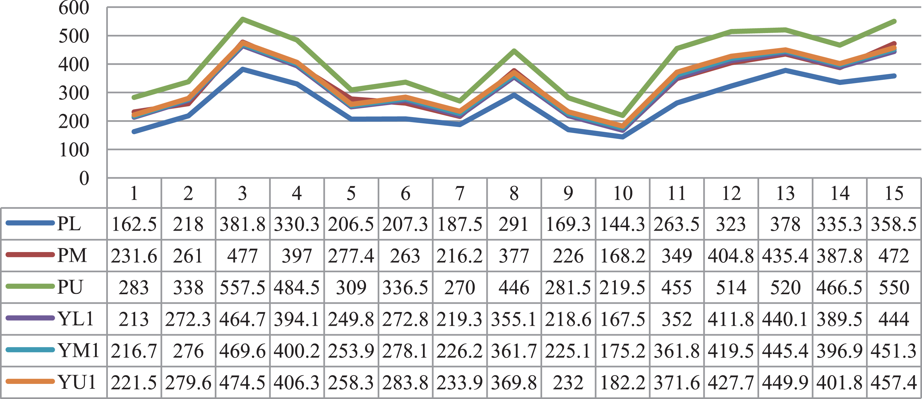
The output of model 1 and the real observations.

Fig.3

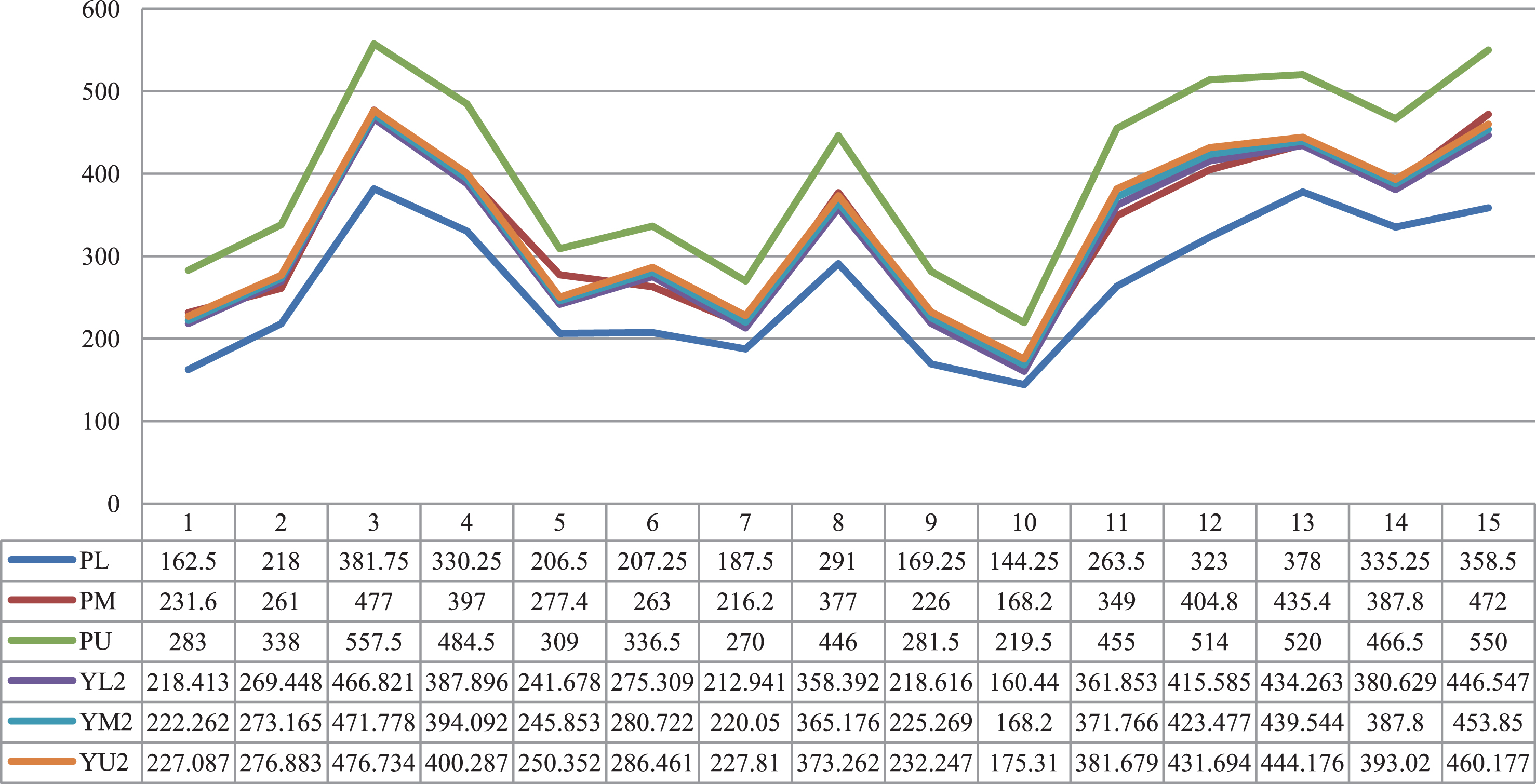
The output of model 2 and the real observations.

Fig.4

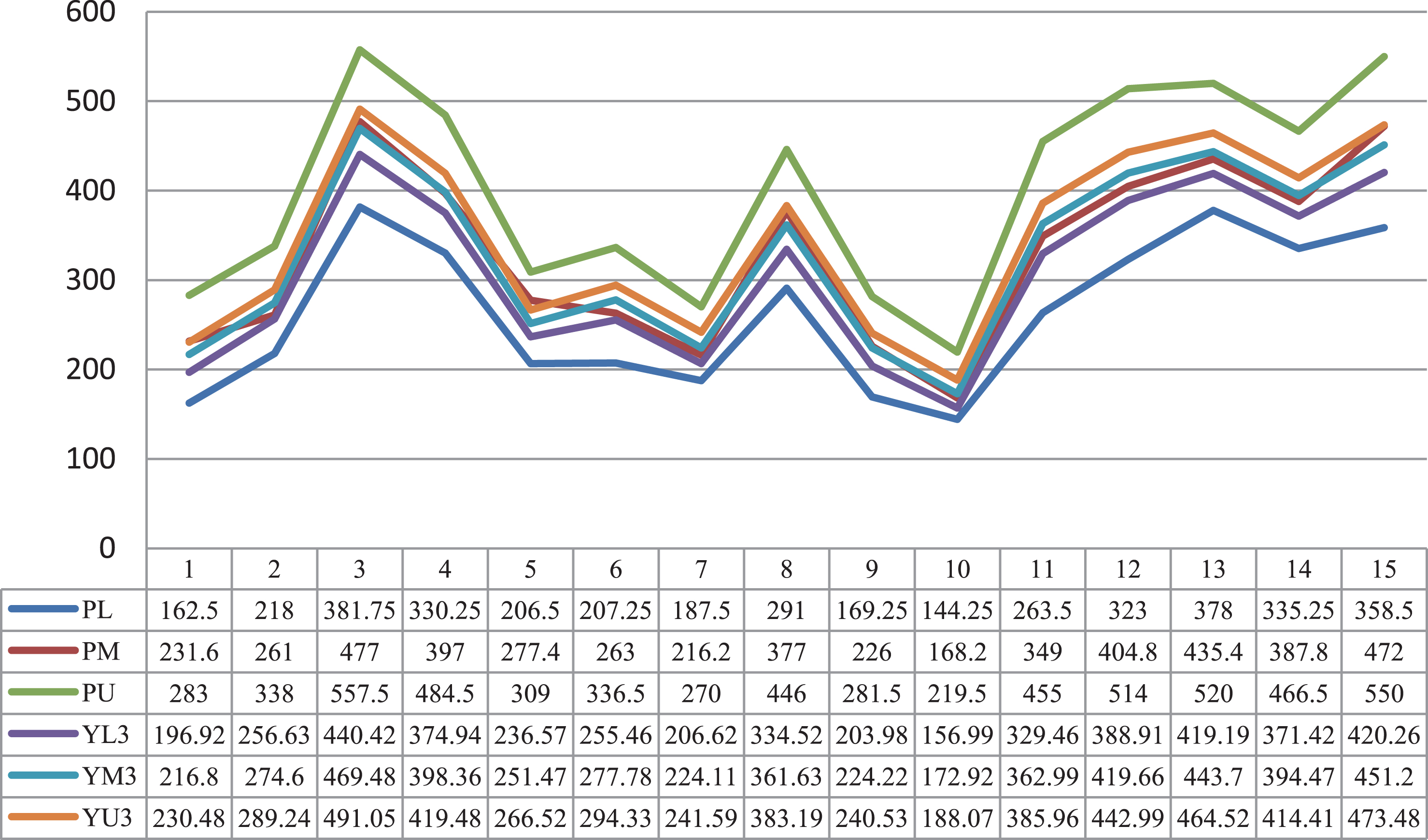
The output of model 3 and the real observations.

Because the input is fuzzy, it is a great advantage for the decision maker to consider real fuzzy distances in her/his fuzzy regression model without any compromise.

4 An introduction to calculate the fuzzy frequency and fuzzy demographic factor for a linguistic term

There are several ways to measure the cardinality of a fuzzy set, extending the classic one in different ways. (Some of them have been employed for calculating the accomplishment of quantified sentences 1 and it is not related to this study.) The most common approaches are the scalar cardinality and the fuzzy cardinality of a fuzzy set. The first approach claims that the cardinality of a fuzzy set is measured by either integer or real means of a scalar value; whereas the second approach assumes the cardinality of a fuzzy set is just another fuzzy set over the non-negative integers. Among the latter, it is common to consider that the cardinality of a fuzzy set must be a fuzzy number, i.e., normalized and convex. Fuzzy numbers are one of the best choices for representing restrictions like linguistic quantifiers, and their arithmetic is that of restrictions.

4.1 Scalar cardinalities

De Luca & Termini [45] who named this as the power of a finite fuzzy set proposed the scalar cardinality. The power of a finite fuzzy set A is given by sum of the membership degrees of the fuzzy set A. Accordingly, the scalar cardinality of fuzzy set

A: Ω⟶ [0, 1] is defined as the sum of the membership degrees of finite fuzzy set A. $| A | = \sum μ_{A} (x), \forall x \in Ω$

|A| is called the sigma- count of A. Zadeh [46], a pioneer of fuzzy sets, investigated the concept of sigma count for fuzzy sets and its applications [47].

The real problem with scalar measures is that they are not really suitable for providing precise information about the cardinality of a fuzzy set. Using a scalar measure of the cardinality is like using a crisp set for representing a fuzzy set. That is, we are losing information for the sake of obtaining a simpler and more easily manageable measure. The problems with this approach are either that it is not always representative, or that it loses too much information.

4.2 Fuzzy cardinalities

“Note that the cardinality of fuzzy sets, especially in the case of finite fuzzy sets, has many applications. Generally, the cardinal theory of fuzzy sets can be used in all situations, where one wants to compare sizes of families of elements satisfying a certain property or to count the number of elements in a family that satisfy a certain property. Whereas, the property is not precisely specified, which means, one cannot surely decide that the property is true or false for considered elements. (e.g. to be young, tall, clever, or rich for certain families of males and females). For instance, measuring sizes of finite fuzzy sets can be used in fuzzy querying in databases, expert systems, evaluation of imprecisely quantified statements, aggregation, decision making in fuzzy environment, metrical analysis of gray images, calculation of histograms of colors and dominant colors [48].”

However, there are many ways of counting fuzzy sets. One of them is introduced as an example where the cardinality of a fuzzy set is defined to be k to a certain degree. According to this approach the fuzzy cardinality of a fuzzy set A is defined by ${| A |}_{f} (k) = μ (k) \land (1 - μ (k + 1)), k = 0, \dots, n .$ where μ(1), μ(2), ... , μ(n) represent the values of μ _A (x1), μ _A (x2), ... , μ _A (xn) arranged in a decreasing order of magnitude and μ(0) = 1, μ(n + 1) = 0.

Example 1 depicts how to calculate the fuzzy frequency for one of the linguistic terms in a specific year based on the fuzzy cardinality.

4.3 Example 1

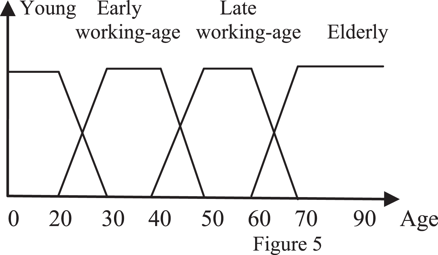
Let the Early working-age population set is defined based on Fig. 5, and the age-structure of the population at the life-stage between t-1 and t follows Table 3. Now, calculation of the fuzzy frequency (the number of elements in the Early working-age population as a fuzzy set) is as follow. (Table 4)

Fig.5
Table 3
The Early working-age set (year t)

Age Population x1000 μ(X) Based on Figure 5 Age Population x1000 μ(X) Based on Figure 5

20 500 0 36 440 1

21 490 0.1 37 430 1

22 490 0.2 38 450 1

23 500 0.3 39 440 1

24 480 0.4 40 440 1

25 500 0.5 41 450 0.9

26 490 0.6 42 460 0.8

27 500 0.7 43 440 0.7

28 490 0.8 44 440 0.6

29 480 0.9 45 470 0.5

30 500 1 46 480 0.4

31 490 1 47 490 0.3

32 500 1 48 490 0.2

33 500 1 49 480 0.1

34 480 1 50 480 0

35 460 1

Table 4
Calculation of the fuzzy frequency

K = Frequency (×10000) 513^* 606^** 701 795 888 985 1081 1180 1278 1375 1473

Poss(|A|_f ≥k) 1 0.9 0.8 0.7 0.6 0.5 0.4 0.3 0.2 0.1 0

^The number of people belong to set of Early working-age* with μ(X) ≥1 i.e. all the people aged 30 to 40. ^**The number of people belong to set of Early working-age with μ(X) ≥0.9 i.e. all the people aged 29 to 41.

From Equation (11), it is concluded that the fuzzy cardinality |A|_f is a fuzzy convex set and the possibility [49] that A has at least k elements is: $Poss ({| A |}_{f} ⩾ k) = {\begin{matrix} μ (k) if k ⩾ j \\ (1 - μ (j)) \lor μ (j), if k < j \end{matrix}$

Where j = ${\begin{matrix} \max {1 ⩽ s ⩽ n | μ (s - 1) + μ (s) > 1}, if A \neq \emptyset \\ 0, if A = \emptyset \end{matrix}$

Note that |A|_f (k) = Poss (|A| = k), where Poss denotes a possibility measure and operator “∨” is a t-conorm (or s-norm) operator e.g. max-operator.

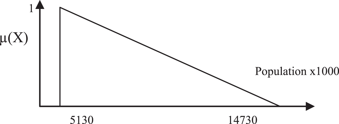
Although the result in Fig. 6 is a discrete fuzzy set, one might use it as a Triangular or LR Fuzzy Number in the model.

Fig.6
A discrete fuzzy set.

In this case, Early working-age at year $t = \tilde{E W_{t}}$ = (5130, 5130, 14730). Figure 7 depicts it as a continuous fuzzy number.

Fig.7
$\tilde{E W_{t}}$ = (5130, 5130, 14730).
5 Real case study – An investigation of the relationship between demographic dynamics and monetary aggregates in Canada and Japan

Age	Population x1000	μ(X) Based on Figure 5	Age	Population x1000	μ(X) Based on Figure 5
20	500	0	36	440	1
21	490	0.1	37	430	1
22	490	0.2	38	450	1
23	500	0.3	39	440	1
24	480	0.4	40	440	1
25	500	0.5	41	450	0.9
26	490	0.6	42	460	0.8
27	500	0.7	43	440	0.7
28	490	0.8	44	440	0.6
29	480	0.9	45	470	0.5
30	500	1	46	480	0.4
31	490	1	47	490	0.3
32	500	1	48	490	0.2
33	500	1	49	480	0.1
34	480	1	50	480	0
35	460	1

5.1 Introduction to demographic studies based on the life-cycle theory

Demographic studies have encompassed a number of various factors since it started in a modern sense in the 17 century by John Graunt. Demographic trends are very smooth, they do not contribute to the short run noise but they are a natural candidate to capture the information that emerges in the long-run. These factors assist researchers to study every kind of dynamic population behaviour and their changes over time. Specific age intervals are noteworthy from economist and financial specialist point of view.

Based on the life-cycle theory [37], a consumer aims to smooth consumption over his lifetime by making appropriate saving/dissaving decisions. As a result, the portfolio choices over different phases of the life-cycle imply a strong imbalance between demand and supply of capital. A number of theoretical models look at the possible link between demographic dynamics and financial asset returns, in particular, the link between age and financial asset returns. Most of these studies claim that a significant relationship between demographic dynamics and asset returns is plausible; however, the magnitude and hence the quantity of this for financial markets are not clear. Therefore, the empirical studies take a leading role in this regard.

According to Roy, et al. [50], school entry age, labor market entry age, age at marriage, age at child-bearing, and retirement age all differ across countries relative to similar cohorts a decade ago. In general, people are spending more years in education, entering the labor force later, delaying marriage and child rearing, and enjoying longer and more uncertain post-retirement periods. As a result, they suggest the need to redefine the age ranges traditionally used to explain asset prices and economic variables in the future.

Moreover, the demographic variables included in the all the previous models were selected in line with other existing empirical work. Most of these empirical studies apply linguistic terms for every different phase of the life cycle (e.g. late working-aged, elderly, adult, and middle-aged) and then define a specific behaviour for each of these cohorts. Although these terms are vague, all the researchers define them as a crisp sets with crisp partitions like 20–40, 40–64, or 65 + . Is it rational to consider that an investor’s behaviour changes at exact ages (i.e., 20, 40, 64, 65), or is a better approach to apply fuzzy sets in order to interpret these linguistic terms?

A list of the different definitions for age intervals, which are considered as independent variables, comes in the following.

Set of three linguistic terms (young, middle age, and old age) and their related ratios [51 –56]

Set of four linguistic terms, People aged 0–14, People aged 15–39, People aged 39–64 years, and People aged 65+ are named young, low middle age, high middle age and old age respectively [57 –60]

Seven age groups with 10-year intervals i.e. (age < 20, 20–29, 30–39, 40–49, 50–59, 60–69, 70 < age) [60 –62]

Fifteen age Groups with 5-year intervals i.e.

(0–4, ... , 70+). [63 –65]

This case study intends to introduce and apply fuzzy sets for the linguistic terms that are mentioned in the life-cycle theory. Consequently, this study has to employ fuzzy frequency for every cohort and develop a fuzzy model based on fuzzy demographic factors. In this real case study, we investigate the impact of the demographic changes on monetary aggregates in Canada and Japan. Moreover, this section deals with a new approach in order to calculate the fuzzy frequency for the linguistic terms, which are applied in demographic studies as independent variables. In particular, this study is based on Nishimura & Takats [33] in which the size of the working-age population during a demographic transition raises the Marshallian K, the ratio of a broad monetary aggregate such as M2 to nominal GDP. This is a real application of the fuzzy input- crisp output case.

To investigate the impact of demography on the money supply, as in Nishimura & Takats [33], we use the following regression for Canada and Japan: $d log K = {\tilde{B}}_{0} + {\tilde{B}}_{1} d log (\tilde{w}) + \hat{ɛ}$ where d log denotes yearly changes in the natural logarithm of the variable in question, K is the Marshallian K, $\tilde{w}$ is the size of the working-age population in terms of TFN. ${\tilde{B}}_{0}$ and ${\tilde{B}}_{1}$ are the fuzzy regression coefficients, in which parameter ${\tilde{B}}_{1}$ depicts the relationship between demography and the money supply.

In order to determine the impact of the size of the working-age population as the fuzzy demographic factor on monetary aggregates in Canada and Japan we follow these steps.

Defining the working-age set as a linguistic term through fuzzy sets

Preparing data

Calculating the fuzzy frequency and fuzzy demographic factors for the linguistic term in each year

Applying the fuzzy regression models 1 to 3,

Solving the models and interpreting the results

5.2 Defining the working-age set as a linguistic term through fuzzy sets

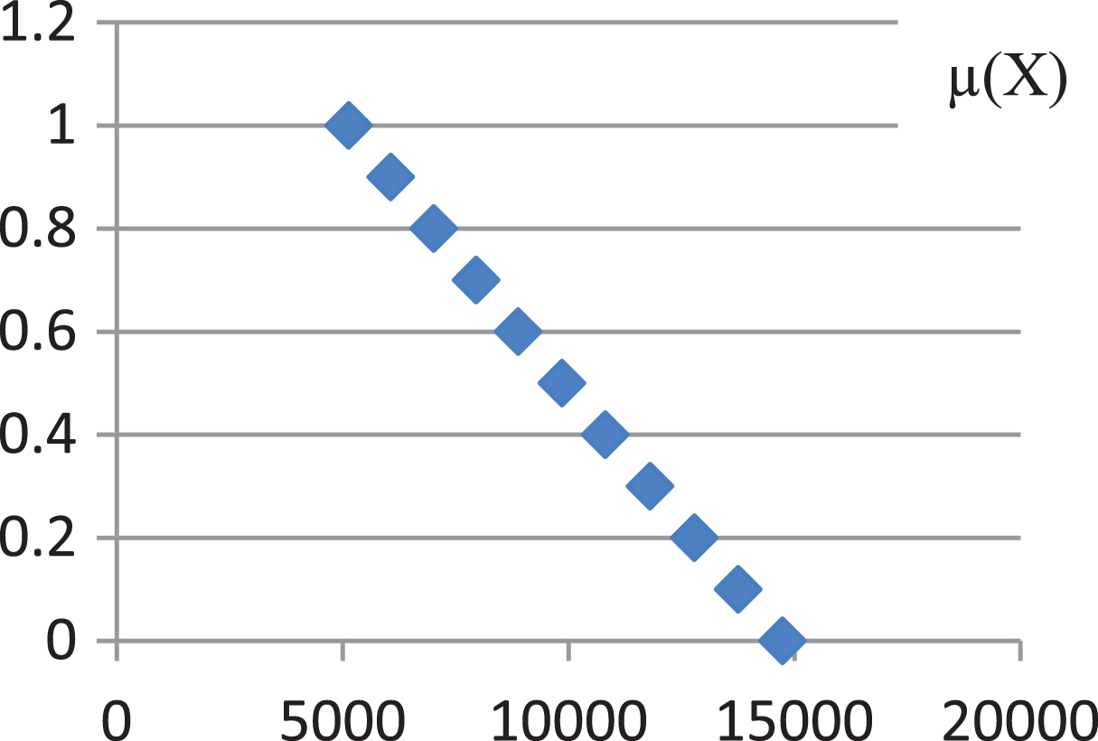
Let X be a linguistic variable with the label “life-cycle” (i.e., the label of this variable is “life-cycle,” and the values of it will be called “Age”) with U = [0, 100]. The terms of this linguistic variable are again fuzzy sets. (They could be called late working-age, elderly, adult, entire, middle-age, and so on.) The base-variable u is the age in years of life. μ(X) is the rule that assigns a meaning, that is a fuzzy set, to the terms. Figure 8, shows the working-age set as a linguistic term through continuous fuzzy sets; however, we calculate them yearly or assume them as TrFNs (Trapezoidal Fuzzy Numbers).

Fig.8

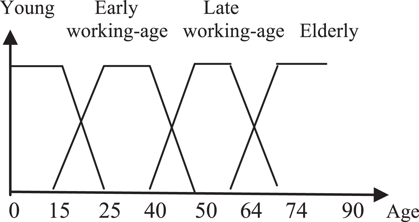
Working-age set = Early working-age set U Late working-age set.

5.3 Preparing data

We use data for the postwar period as it is the longest period available.

Yearly demographic data (1950-2012): come from the UN Population Projections database.

The Marshallian K- the ratio of money supply to nominal economic output M2 (1970-2015 for Canada and 1980-2015 for Japan) is used for the money supply i.e. cash, checking deposits and near money where near money refers to savings deposits, money market securities, mutual funds and other time deposits.

In order to consider economic output, the nominal GDP (current US$) and GDP at market prices (constant 2010 US$) is used. (1960-2015)

We use logarithmic differences in M2 as a percentage of the nominal GDP over the full period

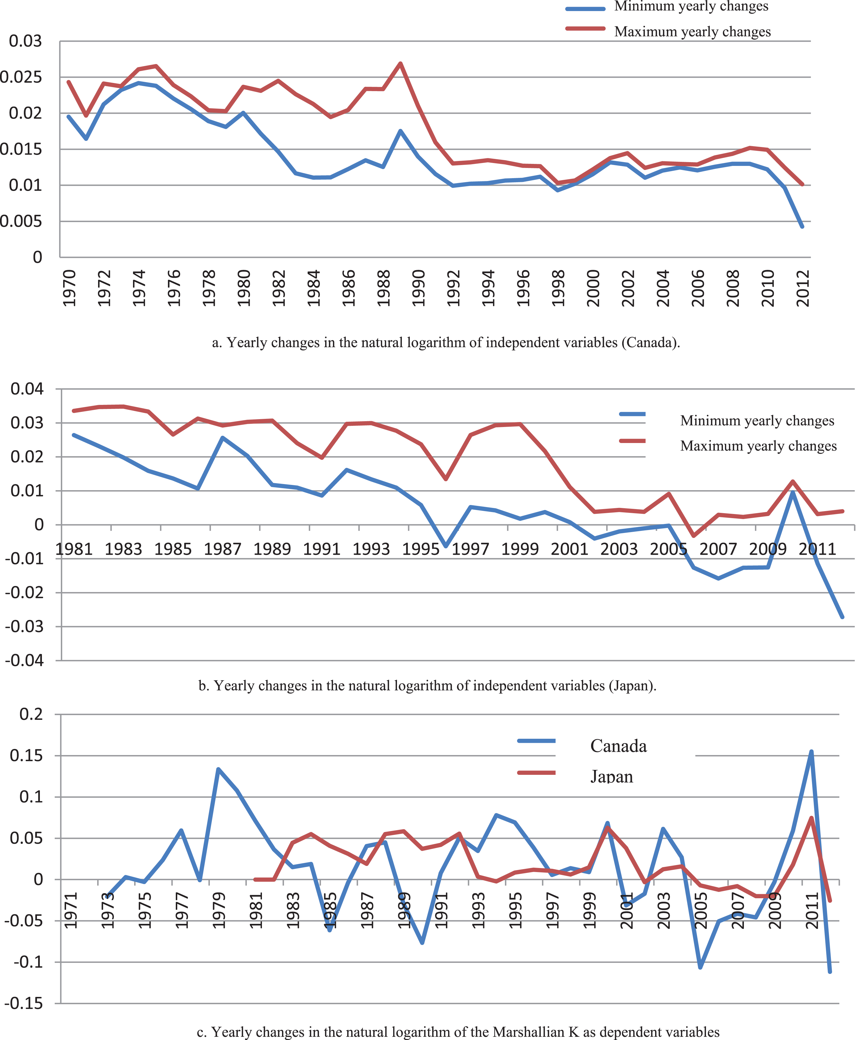
We use data from 1970 to 2012 for Canada and 1980 to 2012 for Japan, which are a common period for all variables. Figure 9-a and 9-b depict yearly changes in the natural logarithm of the fuzzy size of working-age population for Canada, $log (\tilde{w})$ , and the fuzzy size of late working-age population for Japan respectively due to its greater impact on the independent variable. Figure 9c also shows yearly changes in the natural logarithm of the Marshallian K (d log K) for both countries.

Fig.9

a) Yearly changes in the natural logarithm of independent variables (Canada). b) Yearly changes in the natural logarithm of independent variables (Japan). c) Yearly changes in the natural logarithm of the Marshallian K as dependent variables.

5.4 Calculate the fuzzy frequency (fuzzy cardinality 2 ) and fuzzy demographic factors for the linguistic term in each year

To calculate the frequency of the working-age in every year we use the age-structure of the population at the beginning of each year, which is the population at each life-stage between t – 1 and t. Then, it is possible to calculate the fuzzy frequency 3 for the fuzzy sets in our case, working-age. Section 4 clarifies this step through an example, and we provide logarithmic differences of fuzzy population.

5.5 Applying the fuzzy regression models

Using the data prepared as described and the mathematical programming solver LINGO-16, results of the models are shown in Table 5. 4

Table 5
Results of the proposed fuzzy regression models

Model 1 Canada Model 3 Canada Model 1 Japan Model 3 Japan

Crisp coefficient Fuzzy coefficient Crisp coefficient Fuzzy coefficient

$B_{0}^{L}$ = Intercept L - 1.55E-02 - 0.015318

$B_{0}^{M}$ = Intercept M 0.01550188 1.55E-02 0.01531896 0.015318

$B_{0}^{U}$ = Intercept U - 1.55E-02 - 0.015318

$B_{1}^{L}$ - 0.000 - 0.429871

$B_{1}^{M}$ 0.0000 0.000 0.4297768 0.429871

$B_{1}^{U}$ - 0.000 - 0.429871

Maximum d_u 0.1396285 0.1396293 0.6494E-01 0.6473E-01

Objective value 4.62E-03 4.02E-03 9.06E-03 7.25E-02

	Model 1 Canada	Model 3 Canada	Model 1 Japan	Model 3 Japan
$B_{0}^{L}$ = Intercept L	-	1.55E-02	-	0.015318
$B_{0}^{M}$ = Intercept M	0.01550188	1.55E-02	0.01531896	0.015318
$B_{0}^{U}$ = Intercept U	-	1.55E-02	-	0.015318
$B_{1}^{L}$	-	0.000	-	0.429871
$B_{1}^{M}$	0.0000	0.000	0.4297768	0.429871
$B_{1}^{U}$	-	0.000	-	0.429871
Maximum d_u	0.1396285	0.1396293	0.6494E-01	0.6473E-01
Objective value	4.62E-03	4.02E-03	9.06E-03	7.25E-02

Because of using the natural log for the independent and dependent variables in the reference model [33], Triangular Fuzzy Number ${\tilde{B}}_{1} = (B_{1}^{L}, B_{1}^{M}, B_{1}^{U})$ is the elasticity of dependent variable, Marshallian K, with respect to independent variable, fuzzy working-age population. Due to focusing on yearly changes, the results can be seen as strong and dispel concerns about trending variables. Marshallian K is a ratio index and variables that are a proportion or percent are preferred to be used in level form; however, the researchers did not do it in the reference model and we do not either.(Maximum difference (d_u) is related to year 2009 in all models.)

Nishimura & Takats [33] claim that demography does explain a substantial part of the long-run variation in the Marshallian K based on a panel regression analysis. Whereas, in our fuzzy models, there is not a strong evidence for Canada. Neither is there strong evidence using crisp models. On the other hand, demography (late working age) does explain a substantial part of the long-run variation in the Marshallian K for Japan. However, they also mentioned that “in many advanced economies, demographic factors will stop contributing to money supply growth and will start to reduce the Marshallian K.”

In particular, due to the results of Table 5, the elasticity of Marshallian K with respect to fuzzy working-age population is zero $(B_{1} or {\tilde{B}}_{1})$ for Canada. This means that according to the results of these two models and the data from 1970 to 2012, there is not linear relationship between the size of working-age population and monetary aggregates in Canada. In contrast, the elasticity of Marshallian K with respect to fuzzy late working-age population is 0.42 $(B_{1} or {\tilde{B}}_{1})$ for Japan. This means that according to the results of these two models and the data from 1980 to 2012, there is a linear relationship between size of the late working-age population and monetary aggregates in Japan.

In order to figure out a possible relation between Marshallian K as the dependent variable and any characteristic of size of fuzzy working-age population – w_L, w_M, and w_U- as the independent variable, we use three crisp linear regression analyses separately for w_L, w_M, and w_U for and use three crisp linear regression analyses for Japan. Table 6- depicts the results of these analyses. It shows that there are not any significant evidences regarding this relation for Canada but there are significant linear relations for Japan.

Table 6

The results of crisp regression analyses between Marshallian K and w_L, w_M, and w_U

Independent variable	Coefficient B₀	Sig. B₀	Coefficient B₁	Sig. B₁	R	Adjusted R Square
w_LCanada	–0.016	0.579	2.254	0.255	0.179	0.0079
w_MCanada	0.0035	0.902	0.70	0.669	0.0045	–0.020
w_UCanada	0.002	0.94	0.75	0.659	0.0049	–0.0199
w_LJapan	0.0175	.000	0.692	0.0338	0.370	0.109
w_MJapan	0.0128	0.0149	0.640	0.011	0.435	0.163
w_UJapan	.000	0.93	1.0957	0.0020	0.516	0.243

6 Conclusions and remarks

In this paper, we apply a new approach in order to calculate and apply the fuzzy frequency for the linguistic terms related to the size of working-age population, which will be more robust in comparison to the crisp partitions. This approach could be useful for any other demographic factors e.g. school entry age, labor market entry age, age at marriage, age at child-bearing, and retirement age in the economic studies. We have also reviewed the relevant articles on fuzzy linear regression and provided a new approach to determine fuzzy or crisp regression coefficients through three different models based on fuzzy distance. We have applied the models using an example and a case study. Besides the rationality of these models, due to the quadratic programming, our approach matches the observed and predicted values reasonably well.

The results obtained in this work indicate that fuzzy regression with fuzzy distance can effectively enhance forecasting under ambiguities in economic studies. There are several advantages of the proposed methodology. First, the basic principle of the fuzzy distance is rational and simple, yet can provide deep insight into characteristic ambiguity in real data. Secondly, these fuzzy regression models are useful when one faces a combination of crisp and fuzzy data simultaneously. Thirdly, the proposed models do not entail complicated decision-making about selecting the proper objective function. Thus, decision makers are able to trade off between the weights of d_l, d_m, and d_u and select other objective functions in order to lead to improved forecasting results.

We have also presented two fuzzy models that show the demographic changes are not associated with changes in monetary aggregates in Canada but they are in Japan. In particular, the size of the fuzzy working-age population during a demographic transition does not impact on the ratio of money such as M2 to nominal GDP, the Marshallian K for Canada. In contrast, the size of the late fuzzy working-age population during a demographic transition is associated with a change in the ratio of money to GDP for Japan.

Although fuzzy frequency for the linguistic terms constructed in present research for the first time should be helpful in real world problems, a detailed comparative analysis by using other approaches is necessary for solving similar problems of manufacture, finance, economic, and actuarial science area in future.

Footnotes

Acknowledgments

The authors acknowledge the support received from the following sponsors: SSHRC, the Canadian Institute of Actuaries, the Institute and Faculty of Actuaries, the Society of Actuaries, the University of Kent, and the University of Waterloo; as well as the co-applicants for the SSHRC grant: Lori Curtis, Miguel Leon-Ledesma, Jaideep Oberoi, Kathleen Rybczynski, Pradip Tapadar, and Tony Wirjanto.

The authors would like to thank the anonymous reviewers for their constructive suggestions.

¹In Artificial Intelligence, quantified sentences are natural language sentences involving fuzzy linguistic quantifiers, and therefore they express claims about the (fuzzy) quantity or percentage of elements of a (possibly fuzzy) set that verify a certain imprecise property. []

²There is a discussion on some different representations of the cardinality of a fuzzy set and their use in fuzzy quantification. []

³ Determine the number of elements of a set i.e. working-age

⁴Model 2 is not recommended in this special case due to its sensitivity to cases with negligible changes. In this case study, logarithmic periodic change is the dependent variable.

References

Muzzioli

, Ruggieri

and Baets

, A comparison of fuzzy regression methods for the estimation of the implied volatility smile function, Fuzzy Sets and Systems 266 (2015), 131–143.

Tanaka

, Uegima

and Asai

, Linear regression analysis with fuzzy model, IEEE Transactions on Systems, Man, and Cybernetics 12(6) (1982), 903–907.

Shapiro

A.F.

, Fuzzy regression models. Technical Report, Penn State University, US, 2005.

Tanaka

and Watada

, Possibilistic linear systems and their application to the linear regression model, Fuzzy Sets and Systems 27 (1988), 175–289.

Tanaka

, Hayashi

and Watada

, Theory and methodology-Passibilistic linear regression analysis for fuzzy data, European Journal of Operational Research 40 (1989), 389–396.

Yen

, Ghoshray

and Roig

, A linear regression model using triangular fuzzy number coefficients, Fuzzy Sets and System 106(2) (1999), 167–177.

Pushpa

and Vasuki

, A least absolute approach to multiple fuzzy regression using Tw-norm based operations, International Journal of Fuzzy Logic Systems 3(2) (2013a), 73–84.

Diamond

, Fuzzy Least Squares, Information Sciences 46 (1988), 141–157.

Savic

D.A.

and Pedrycz

, Evaluation of fuzzy linear regression models, Fuzzy Sets and Systems 39(1) (1991), 51–63.

10.

D’Urso

, Massari

and Santoro

, Robust fuzzy regression analysis, Information Sciences 181 (2011), 4154–4174.

11.

Kim

and Bishu

R.R.

, Evaluation of fuzzy linear regression models by comparing membership functions, Fuzzy Sets and Systems 100(1-3) (1998), 343–352.

12.

Wang

H.F.

and Tsaur

, Resolution of fuzzy regression model, European Journal of Operational Research 126(3) (2000), 637–650.

13.

Ishibuchi

and Nii

, Fuzzy regression using asymmetric fuzzy coefficients and fuzzified neural networks, Fuzzy Sets and Systems 119(2) (2001), 273–290.

14.

Guoa

and Tanaka

, Dual models for possibilistic regression analysis, Computational Statistics & Data Analysis 51 (2006), 253–266.

15.

Pushpa

and Vasuki

, Estimation of Confidence Level ‘h’ in Fuzzy Linear Regression Analysis using Shape Preserving Operations, International Journal of Computer Applications 68(17) (2013b), 0975–8887.

16.

Sakawa

and Yano

, Multiobjective fuzzy linear regression analysis for fuzzy input–output data, Fuzzy Sets and Systems 47(2) (1992), 173–181.

17.

D’Urso

, Linear regression analysis for fuzzy/crisp input and fuzzy/crisp output data, Computational Statistics & Data Analysis 42(1-2) (2003), 47–72.

18.

Hojati

, Bector

C.R.

and Smimou

, A simple method for computation of fuzzy linear regression, European Journal of Operational Research 166(1) (2005), 172–184.

19.

Sohn

S.Y.

, Kim

D.H.

and Yoon

J.H.

, Technology credit scoring model with fuzzy logistic regression, Applied Soft Computing 43 (2016), 150–158.

20.

Bargielaa

, Pedryczb

and Naka

, Multiple regression with fuzzy data, Fuzzy Sets and Systems 158 (2007), 2169–2188.

21.

Bertoluzza

, Corral

and Salas

, On a new class of distances between fuzzy numbers, Mathware & Soft Computing 2 (1995), 71–84.

22.

Chen

L.-H.

and Hsueh

C.-C.

, Fuzzy Regression Models Using the Least-Squares Method Based on the Concept of Distance, IEEE Transactions on Fuzzy Systems 17(6) (2009), 1259–1272.

23.

Chen

S.-P.

and You

S.-S.

, A Fuzzy Linear Regression Model Based on Dissemblance Index, International Journal of Mathematical, Computational, Physical, Electrical and Computer Engineering 8(9) (2014), 1278–1283.

24.

Icen

and Cattaneo

, Different distance measures for fuzzy linear regression with Monte carlo methods, Soft Computing, 2016.

25.

De Hierro

A.F.R.L.

, Martínez-Moreno

and Aguilar-Peña

Estimation of a Fuzzy Regression Model Using Fuzzy Distances, IEEE Transactions on Fuzzy Systems 24(2) (2016), 344–359.

26.

Zeng

, Merigó

J.M.

, Palacios-Marqués

, Jin

and Gu

, Intuitionistic fuzzy induced ordered weighted averaging distance operator and its application to decision making, Journal of Intelligent & Fuzzy Systems 32(1) (2017), 11–22.

27.

, Chang

, Cao

and Liang

, A trust propagation and collaborative filtering based method for incomplete information in social network group decision making with type-2 linguistic trust, Computers & Industrial Engineering, 2018a.

28.

Zeng

, Mu

and Baležentis

, A novel aggregation method for Pythagorean fuzzy multiple attribute group decision making, Journal of Intelligent & Fuzzy Systems 33 (2018), 573–585.

29.

Zeng

, Pythagorean Fuzzy Multiattribute Group Decision Making with Probabilistic Information and OWA Approach, Journal of Intelligent & Fuzzy Systems 32(11) (2017), 1136–1150.

30.

, Sun

, Fujita

and Chiclanac

, An attitudinal consensus degree to control the feedback mechanism in group decision making with different adjustment cost, Knowledge-Based Systems 164 (2019), 265–273.

31.

Zeng

and Xiao

, A method based on topsis and distance measures for hesitant fuzzy multiple attribute decision making, Technological and Economic Development of Economy 24(3) (2018), 905–919.

32.

, Chiclana

and Liao

, Isomorphic Multiplicative Transitivity for Intuitionistic and Interval-Valued Fuzzy Preference Relations and Its Application in Deriving Their Priority Vectors, IEEE Transactions on Fuzzy Systems 26 (2018b), 193–202.

33.

Nishimura

K.G.

and Takáts

, Ageing, property prices and money demand, Bank for International Settlements, 2012.

34.

Voxman

, Some remarks on distances between fuzzy numbers, Fuzzy Sets and Systems 100(1-3) (1998), 353–365.

35.

Chakraborty

and Chakraborty

, A theoretical development on a fuzzy distance measure for fuzzy numbers, Mathematical and Computer Modelling 43(3-4) (2006), 254–261.

36.

Sadi-Nezhad

, Noroozi-yadak

and Makui

, Fuzzy Distance of Triangular Fuzzy Numbers, Journal of Intelligent & Fuzzy Systems 25(4) (2013), 845–852.

37.

F. Modigliani, and R. Brumberg, Utility analysis and the consumption function: An interpretation of cross-section data, (Rutgers University Press, New Brunswick): K. Kurihara, ed.: Post Keynesian Economics, 1954.

38.

Sadi-Nezhad

, Khalili-Damghani

and Norouzi

, A new fuzzy clustering algorithm based on multi-objective mathematical programming, TOP 23(1) (2015), 168–197.

39.

Shahsamandi

, Sadi-nezhad

E.S.

and Saghaei

, Multi-objective complete fuzzy clustering approach, Intelligent Automation & Soft Computing 23(2) (2017), 285–294.

40.

Chen

S.J.

and Hwang

C.L.

, Fuzzy Multiple Attribute Decision Making, Methods and Applications, Berlin: Springer, 1992.

41.

Branke

, Deb

, Miettinen

and Słowivinski

, Multiobjective Optimization- Interactive and Evolutionary Approaches, Germany:, Springer-Verlag Berlin Heidelberg, 2008.

42.

Yao

, Xu

and Guo

, A Stone Resource Assignment Model under the Fuzzy Environment, Mathematical Problems in Engineering, 2012.

43.

, Hou

, Yao

and Li

, Integrated waste load allocation for river water pollution control under uncertainty: A case study of Tuojiang River, China, Environmental Science and Pollution Research 24(21) (2017), 17741–17759.

44.

Hashim

, Nazam

, Yao

, Baig

S.A.

, Abrar

and Zia-ur

, Application of multi-objective optimization based on genetic algorithm for sustainable strategic supplier selection under fuzzy environment, Journal of Industrial Engineering and Management 10(2) (2017), 188–212.

45.

De Luca

and Termini

A definition of a nonprobabilistic entropy in the setting of fuzzy sets theory, Inform and Control 20 (1972), 301–312.

46.

Zadeh

L.A.

, A computational approach to fuzzy quantifiers in natural languages, Computing and Mathematics with Applications 9 (1983), 149–184.

47.

Zimmerman

H.J.

, Fuzzy Set Theory and Its Applications, Springer Science & Business Media, 2001.

48.

Holčapek

, A graded approach to cardinal theory of finite fuzzy sets, part I: Graded equipollence, Fuzzy Sets and Systems 298 (2016), 158–193.

49.

Quirós

, Alonso

, Díaz

and Montes

, On the use of fuzzy partitions to protect data, Integrated Computer-Aided Engineering 21 (2014), 355–366.

50.

Roy

, Punhani

and Shi

, How demographics a prices global demographics and pensions, Credit Suisse, 2012.

51.

Davis

E.P.

and Li

Brunel University, Economics and Finance Working papers, Demographics and financial asset prices in the major industrial economies., 2003.

52.

Brunetti

and Torricelli

, Demographics and asset returns: Does the dynamics of population ageing matter?, Annals of Finance 6(2) (2010), 193–219.

53.

Ang

and Maddaloni

, Do demographic changes affect risk premiums? Evidence from international data, Working paper No.208, European Central Bank, 2003.

54.

Davis

E.P.

, How will ageing affect the structure of financial market? in, RBA Annual Conference, Reserve Bank of Australia, 2006.

55.

Huynh

, Mallik

and Hettihewa

, The impact of macroeconomic variables, demographic structure and compulsory superannuation on share prices: The case of australia, Journal of International Business Studies 37(5) (2006), 687–698.

56.

Lee

K.F.

, Demographics and the long-horizon returns of dividend yield strategies, The Quarterly Review of Economics and Finance 53(2) (2013), 202–218.

57.

Geanakoplos

, Magill

and Quinzii

Demography and the longrun predictability of the stock market, Brookings Papers on Economic Activity (1) (2004), 241–325. https://muse.jhu.edu/ (accessed February 11, 2018)., 2004.

58.

Park

and Rhee

, Population aging and financial markets: Across-country study, Seoul Journal of Economics 20(3) (2007), 333–354.

59.

J. Poterba, The impact of population aging on financial markets NBER Working Paper No. 10851, 10 2004., NBER Working Paper No. 10851, 10 2004, 2004.

60.

Favero

C.A.

, Gozluklu

A.E.

and Tamoni

, Demographic trends, the dividend-price ratio, and the predictability of long-run stock market returns, Journal of Financial and Quantitative Analysis 46(11) (2011), 1493–1520.

61.

Favero

C.A.

, Gozluklu

A.E.

and Yang

, Demographics and the behavior of interest rates, IMF Economic Review 64(4) (2016), 732–776.

62.

Bovbjerg

B.D.

and Scott

G.A.

, Baby boom generation, retirement of baby boomers is unlikely to precipitate dramatic decline in market returns, but broader risks threaten retirement security, Report to Congressional Committees, United States Government Accountability Office, 7, 2006. No:GAO-06-718., USA, 2006.

63.

Arnott

R.D.

and Chaves

D.B.

, Demographic changes, financial markets, and the economy, Financial Analysts Journal 68(1) (2012), 23–46.

64.

Brooks

, Demographic Change and Asset Prices, in RBA Annual Conference Reserve Bank of Australia, June 2006., Australia, 2006.

65.

Ratanabanchuen

England: PhD thesis, Department of Management of The London School of Economics and Political Science, Demographic Transition, Pension Schemes investment, and the Financial Market., 2013, 2013.

66.

Chamorro-Martínez

, Sánchez

and Soto-Hidalgo

J.M.

, A discussion on fuzzy cardinality and quantification. Some applications in image processing, Fuzzy Sets and Systems 257(16) (2014), 85–101.

K = Frequency (×10000)	513^*	606^**	701	795	888	985	1081	1180	1278	1375	1473
Poss(\|A\|_f ≥k)	1	0.9	0.8	0.7	0.6	0.5	0.4	0.3	0.2	0.1	0