Artificial neural networks approaches for predicting the potential for hydropower generation: a case study for Amazon region

Abstract

This study both presents a novel methodology and compares the performance of computational intelligence techniques for the predictive modeling of the monthly potential for hydropower generation. Two different approaches are employed to forecasting energy generation: polynomial neural network and conventional artificial neural network (ANN). The first one technique is a deep learning type named group method of data handling (GMDH). And the second one is the multilayer perceptron (MLP) feed forward with back-propagation algorithm. The ANN dealt with two different optimization algorithms for training the model: Levenberg-Marquardt and Bayesian regulation. Rainfall data are used as inputs to feed the models. The performance of each model is scrutinized based on three statistical performance criteria. The results found that the computational intelligence techniques can model the dynamic, seasonal and non-linear behavior of the studied issue. The predictions from the GMDH method resulted in slightly better accuracy than the values obtained by the conventional ANN. The analyzes also showed that the values that determine the steady energy of the hydropower plant are well captured by the models. This feature makes the model an important tool for energy planning and decision making.

Keywords

GMDH artificial neural network hydropower generation Amazon region

1 Introduction

Energy is fundamental to development. Each country uses its natural resources for energy generation. In many countries the matrix for electricity generation is highly dependent on water sources. In Brazil, e.g. 68% of the electric energy comes from hydropower plants [1]. Often the implementation of a hydropower plant is necessary, however it can cause significant environmental and social impacts [2, 3].

In the second half of the last century, Brazil deployed several plants with accumulation reservoirs, that is, those that form a bulky and very extensive lake, and thus allow the regularization of monthly or annual flow. However, because environmental reasons, currently the new hydropower plants projects consider only dams with no reservoirs or very small reservoirs, so that the water stored is significantly smaller and allows only the regularization of daily or weekly flow [4 –6]. This kind of hydropower plant is named run-of-the-river scheme and because it has small reservoirs, the energy production is more susceptible to climate variability [7, 8]. For this reason, a run-of-the-river plant becomes very dependent on the natural flows of the river, which has a seasonal behavior, and therefore, during the dry season, suffer a significant reduction of the power generation. This characteristic makes it imperative to correctly determine the critical period that corresponds to the lowest energy generation and should define the steady energy of the plant, i.e. the maximum continuous power production.

Regarding the preliminary feasibility studies of a hydropower plant, which is a necessary component for the implementation of power plant designs [4, 6], an important approach of this study is the estimation of the potential for power generation. The main parameters employed to determine the amount of electric energy that a hydropower plant can generate are the river flow and the hydraulic head [7, 9, 10]. Although the hydraulic head is an engineering parameter dependent on the relief and the design of the plant, the traditional method for assessing the potential of a hydropower plant (HPP) considers the time series of a long-term flow measurements carried out using hydrological stations data.

In Brazil, the last frontier for the exploitation of hydroelectric energy is the Amazon region, where is estimated that more than 50% of the Brazilian potential for hydroelectric is found [11]. Therefore, in the next years, the implementation of several hydropower plants in the region is foreseen. The Brazilian regulation requires that previous studies for the implantation of a HPP employ discharge measurement data (flow) for a seventy-year time series, in order to capture with statistical security, the dry periods that define the steady energy [12]. However, many times is quite common there is no long-term streamflow dataset for the Amazonian rivers, and this can be a limiting factor for the estimation of the potential for hydropower generation with the necessary degree of confidence. Moreover, this can also compromise the success of the project that involves high amounts of financial resources and whose environmental and social impacts are extremely important, demanding maximum rigor for the project planning [13].

Regarding the difficulties frequently encountered in the Amazon region about hydrological data record, this work aims to present a methodology applied to the modeling of the monthly potential for hydropower generation using rainfall time series to aid in decision making before the implementation of hydropower plants projects. The atmospheric variables present a high complexity due their non-linear characteristics, that is why the chosen approach to modeling is the artificial intelligence.

The use of artificial intelligence techniques to solve complex problems has been very promising. In this sense, the present study also aims to perform a comparative analysis between the performance of both polynomial and conventional neural networks. The polynomial neural network employed in this study is a deep learning type named group method of data handling (GMDH). Since this method does not require prior knowledge of the expert to select the variables most relevant for use in the model entry layer, it is quite suitable for practical applications. In general, as the artificial neural networks (ANN) are suitable for small sample size learning [14], the multilayer perceptron (MLP) is also used. And the back-propagation algorithm (BPA) is used too, because for supervised training, the BPA can recursively adjust weights and biases to minimize error. The proposed methodology is demonstrated for a section of the Tapajós River, in the municipality of Itaituba, state of Pará, where the Brazilian government intends to install a Hydropower Plant (HPP) named Jatobá.

2 Machine Learning and Related Works

2.1 Group method of data handling (GMDH)

In the last decade, the use of computational intelligence techniques for modeling and predicting loads in power systems has been increasingly frequent [15] and one of the most promising methods that have shown promising results is the Group Method of Data Handling (GMDH). This approach is generally applied to short-term load forecasting [16 –19] or modeling and forecasting of electricity consumption [20, 21]. There are many applications to diagnose and predict plant failure [22, 23], as well as to forecast rainfall [14] and stream flow [24], but this method has not yet been sufficiently explored and applied to predictive modeling of the potential for hydropower generation, especially in the Amazon region.

The pioneer of the GMDH technique was Ivakhnenko [25], but several other scientists carried out subsequent contributions and significant developments. GMDH consists of an inductive and self-organizing approach to mathematical modeling of complex systems [26]. This method is a robust and versatile technique and also considered appropriate to solve artificial intelligence problems such as identification, short and long-term prediction of random processes and recognition of patterns in complex systems [14 , 28].

The characteristics presented by the GMDH and its diversity of uses are the features that lead the use of this algorithm for application in this methodology. Moreover, for selecting the most relevant input variables, due the ability to avoid problems with overfitting, and for objectively selecting the optimal model, all those advantages favored their choice.

The fundamental concept of the GMDH approach is to structure a feedforward multi-layered neural network, using hierarchically connected partial models, so that the best models can be selected through appropriate methods, and the bad models are discarded [29, 30]. Each layer consists of input variables pairs and one output variable (Fig. 1).

Fig.1

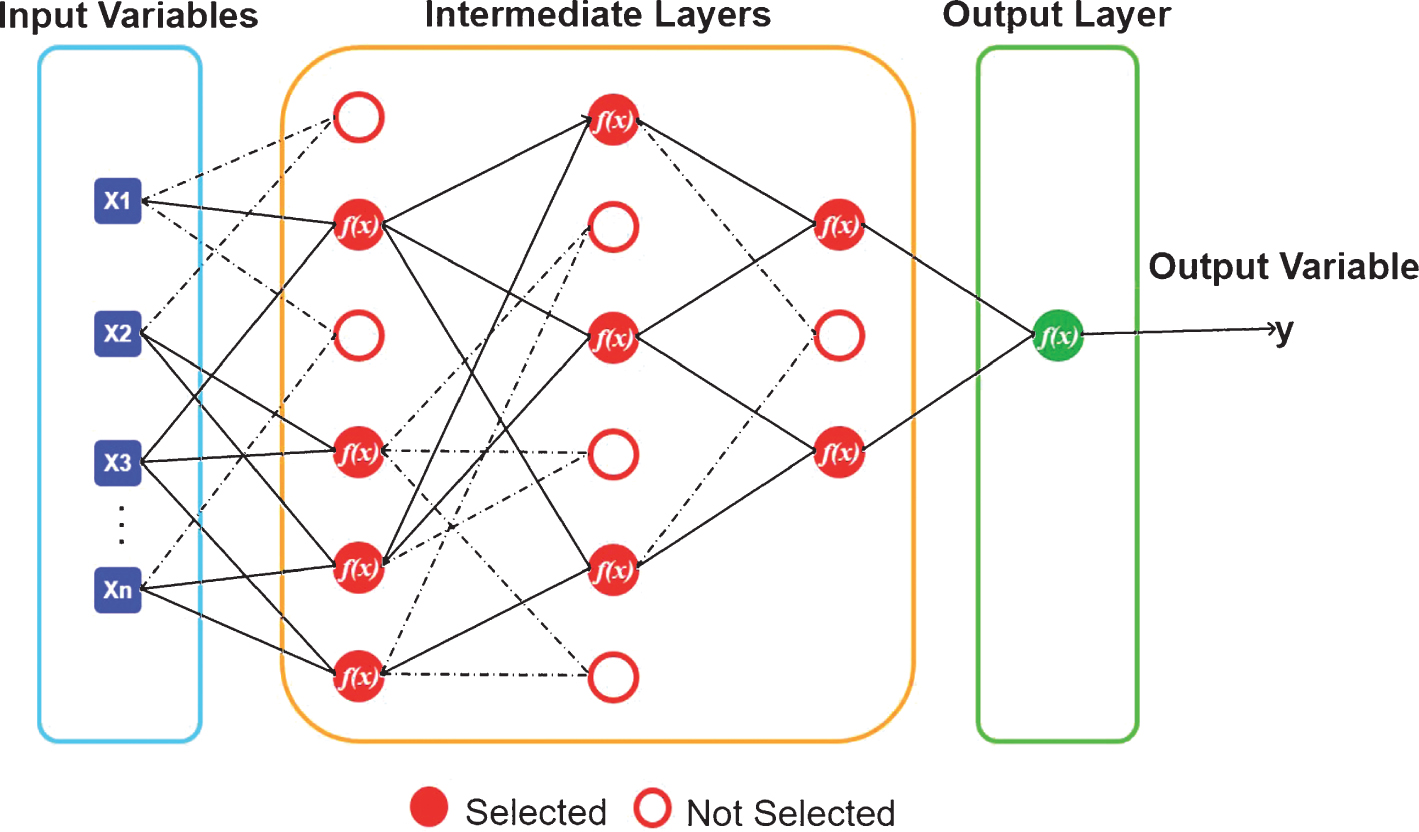
General architecture for a GMDH-type network.

The general mathematical formulation that solves the connections between input and output variables can be explained by the polynomial function theory named Kolmogorov-Gabor polynomials [31, 32]:

$\begin{matrix} y = a_{0} + \sum_{i = 1}^{n} a_{i} x_{i} + \sum_{i = 1}^{n} \sum_{j = 1}^{n} a_{i} a_{j} x_{i} x_{j} + \\ + \sum_{i = 1}^{n} \sum_{j = 1}^{n} \sum_{k = 1}^{n} a_{i} a_{j} a_{k} x_{i} x_{j} x_{k} + . . . \end{matrix}$ (1) where X = (x₁, x₂, …, x_n) is the input vector and y is the output variable. In this way, a complete description can be simplified by a system of partial quadratic polynomials with only two variables, as follows: $\overset{⌢}{y} = w_{0} + w_{1} x_{1} + w_{2} x_{2} + w_{3} x_{1}^{2} + w_{4} x_{1} x_{2} + w_{5} x_{2}^{2}$ (2) where x₁ and x₂ are the input variables, $\overset{⌢}{y}$ is the output variable (target), and w₀, . . . , w₅ are parameters (weights).

In each set of learning data which includes both the dependent variable y, as well as the independent variables x₁, x₂, . . . , x_n, the data sample is separated into training subset and test subset. From the n input variables, combinations using two variables are generated for all input variables, to form pairs that constitute the units that will integrate the first layer. For all units are estimated some weights parameters using the training subset.

A criterion is defined as a comparison metric between the partial models and the expected result, to select the best partial models, discarding those that do not meet the criterion of choice. The selected partial models become part of the first layer, and the predictions of the first layer units are set as new input variables that will feed the next layer and thus build a multilayer structure by applying the previous steps. When the selection criterion of the partial models is no longer met, the addition of new layers is finished and the unit of least error in the highest order layer is chosen as the final model.

2.2 Multilayer perceptron (MLP) / back-propagation algorithm (BPA)

In general, a neural network can be understood as a structure formed by a set of interconnected processing units, in which each processing unit, named an artificial neuron, has an activation function [33]. Multilayer Perceptron (MLP) consists of a type of feed forward neural network composed by an input layer and output layer, in addition to at least one layer of intermediate neurons, named the hidden layer, which is responsible for the nonlinearity of the MLP networks allowing that be able to solve complex problems, just like the real problems [34], as showed in the Fig. 2.

Fig.2

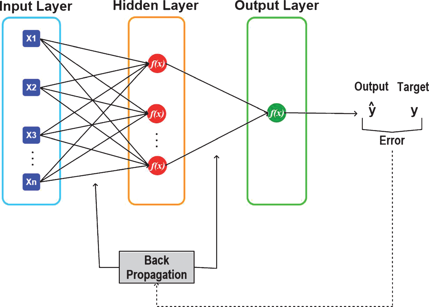
– MLP scheme with back-propagation algorithm.

The training of the MLP networks requires the use of an algorithm that allows to establish an optimal set of weights for the network. The most widely used learning algorithm for non-linearly separable tasks is error back-propagation algorithm (BPA) [35, 36]. The problem encountered during the training of an MLP is that with the inclusion of one or more intermediate layers, the error of these layers is not known, although it is necessary to adjust the weights. But this issue can be solved with BPA, which performs a recursive propagation of errors.

As learning is supervised, the goal of BPA is to adjust weights so that the error between the desired and calculated output is minimized. This process occurs from the error between the sample pairs of input and output ANN data, consisting of two phases: forward and backward. The forward phase is used to find an output from the input values of a given pattern, that is, the signals are propagated in the progressive sense (from the input layer to the output layer), finding the signal output and error, but keeping the weights fixed. The backward phase compares this output with the desired output and recursively updates (from the output layer to the input layer) the values of the weights of the connections of the neurons of the structure [33, 35]. The error is determined according to the rule of weight adjustment (generalized delta rule) [37, 38]: $E = 1 / 2 \sum_{i = 1}^{p} \sum_{j = 1}^{n} {(d_{j}^{i} - y_{j}^{i})}^{2}$ (3) where p is the number of patterns used in training, n is the number of outputs, d is the desired output, and y is the estimated output. The weight update after calculation of error E is given by the following expression: $W = W - α \frac{\partial E}{\partial W}$ (4) where α represents the training rate.

BPA can be applied to any network that uses a differentiable activation function and supervised learning, being based on the gradient descent. The training process is performed based on trial and error, so one of the problems of the algorithm is its training time. The rate of updating of weights is what influences this time. If the set rate is too low, the network consumes too much time for training. On the other hand, if the rate is high, the network can converge in a short time interval, but when another input is presented, the network may become unstable, resulting in unreliable results. For this reason, this work tested the application of two algorithms for BPA optimization: Levenberg-Marquardt and Bayesian regulation.

2.3 Levenberg-Marquardt algorithm

While the standard back-propagation uses the gradient descent as a method of approximation the minimum of the error function, the Levenberg-Marquardt (LM) algorithm uses a Newton approximation [39]. This approximation is obtained from the modification of the Gauss-Newton method by introducing the parameter μ, according to the equation: $W_{n + 1} = W_{n} - {(J_{n}^{T} J_{n} + μ I)}^{- 1} J_{n}^{T} E_{n}$ (5) where W is the weight, I is an identity matrix, E is the error and J is the Jacobian matrix. The parameter μ is a non-negative scalar multiplied by a factor (β) whenever a step results in an increase in the error function, which is to be minimized. When a step results in a decrease in the performance function, μ is divided by the β factor. This means that if there is a convergence to the minimum of the function, μ is small and the algorithm approaches Newton’s method (step 1/μ); in case of no convergence, the method approaches the gradient descent. Thus, the Levenberg-Marquardt algorithm combines the best features of two numerical methods. The parameter μ acts as a training stabilization factor, adjusting the approximation to use the fast convergence of the Newton method and avoiding very large steps that may lead to a convergence error [39]. Newton’s method is faster and more accurate to achieve the minimum error, so the goal of the Levenberg-Marquardt algorithm is to move to Newton’s method as fast as possible [40].

2.4 Regulation Bayesian algorithm

Regularization is a generic name for methods involving the modification of the performance function of neural networks, which is usually the sum of the squares of training errors, and aims to improve its generalization capacity [41]. Eventually, data used as input from a neural network may not be as clean as desirable, and such a noisy condition may lead the training data set to an overfitting. Thus, the approach employing Bayesian regularization can improve the generalization ability of the neural network and present a better model performance. In the Bayesian approach the performance function can be optimized by treating the synaptic weights and biases of the network as random variables with specific distributions, such that the objective function F is defined as $F = γ E_{D} + (1 - γ) E_{W}$ (6) where E_D is the sum of the quadratic errors, E_W = ||w||2/2 is the sum of the squares of the network parameters, and γ is the performance ratio whose magnitude determines the training emphasis. This type of performance function forces a reduction in the values of the weights and consequently leads to a reduction of the overfitting. However, another problem is the determination of the optimal value for the coefficient γ. Since γ must be in the range 0 ≤ γ ≤ 1, if there is an increase in the value of the performance ratio above the required, an overfitting may occur; on the other hand, if the ratio is too small, the network will not be properly tuning the training data[42].

The Bayesian structure is a technique that allows to automatically determine the optimum parameter. This method causes the parameter to be selected using only the training data, without having to use separate training and validation data. The Bayesian structure considers a probability distribution over the weighting space, representing the relative degrees of reliability in different values for the weights. The weight space is initially assigned to some previous distribution. Let D ={ x_m, t_m } the training data set of the target input pair. After the data are obtained with the Gaussian additive noisy assumed at the target values, the posterior probability distribution for the weight p (w|D, γ) of the ANN can be updated according to the Bayes rule: $p (w | D, γ) = \frac{p (D | w, γ) p (w | γ)}{p (D | γ)}$ (7) where p (w|γ) is the prior distribution, p (D|w, γ) is the probability function and p (D|γ) is the normalization factor, which guarantees that the total probability is 1. In the Bayesian structure, the optimal weight should maximize the posterior probability p (w|D, γ) which is equivalent to minimizing the function in Equation (6). The performance ratio parameter γ is optimized by applying the Bayes rule $p (γ | D) = \frac{p (D | γ) p (γ)}{p (D)}$ (8)

If a uniform prior density p (γ) is assumed for the regularization parameter γ, then the posterior probability maximization is obtained by maximizing the probability function p (D|γ). Since all probabilities have a Gaussian form, it can be expressed as $p (D | γ) = {(\frac{π}{γ})}^{- N / 2} {(\frac{π}{1 - γ})}^{- L / 2} Z_{F} (γ)$ (9) where L is the total number of parameters in the neural network. If F has a single minimum as a function of w in w^* and is in the form of a quadratic function in a small area surrounding the point, Z_F is approximated as $Z_{F} = {(2 π)}^{L / 2} \det^{- 1 / 2} H^{*} exp [- F (w^{*})]$ (10) where H = γ ∇ ²E_D + (1 - γ) ∇ ²E_W is the Hessian matrix of objective function. Substituting the value of Z_F from Equation (10) to Equation (9), the optimal value of γ at the minimum point can be determined [43]. However, a disadvantage of the Bayesian approach is that it requires the computation of the Hessian matrix of the performance index. But using the Gauss-Newton approximation for the Hessian matrix, the additional overhead for Bayesian regularization is minimal when the Levenberg-Marquardt optimization algorithm is employed to locate optimal weights. Thus, the Bayesian regulation algorithm provides a good generalization of the network.

3 Methodology

The flowchart of the process that defines the general methodology for developing the non-physical models to simulate the potential for hydropower generation is presented in Fig. 3.

Fig.3

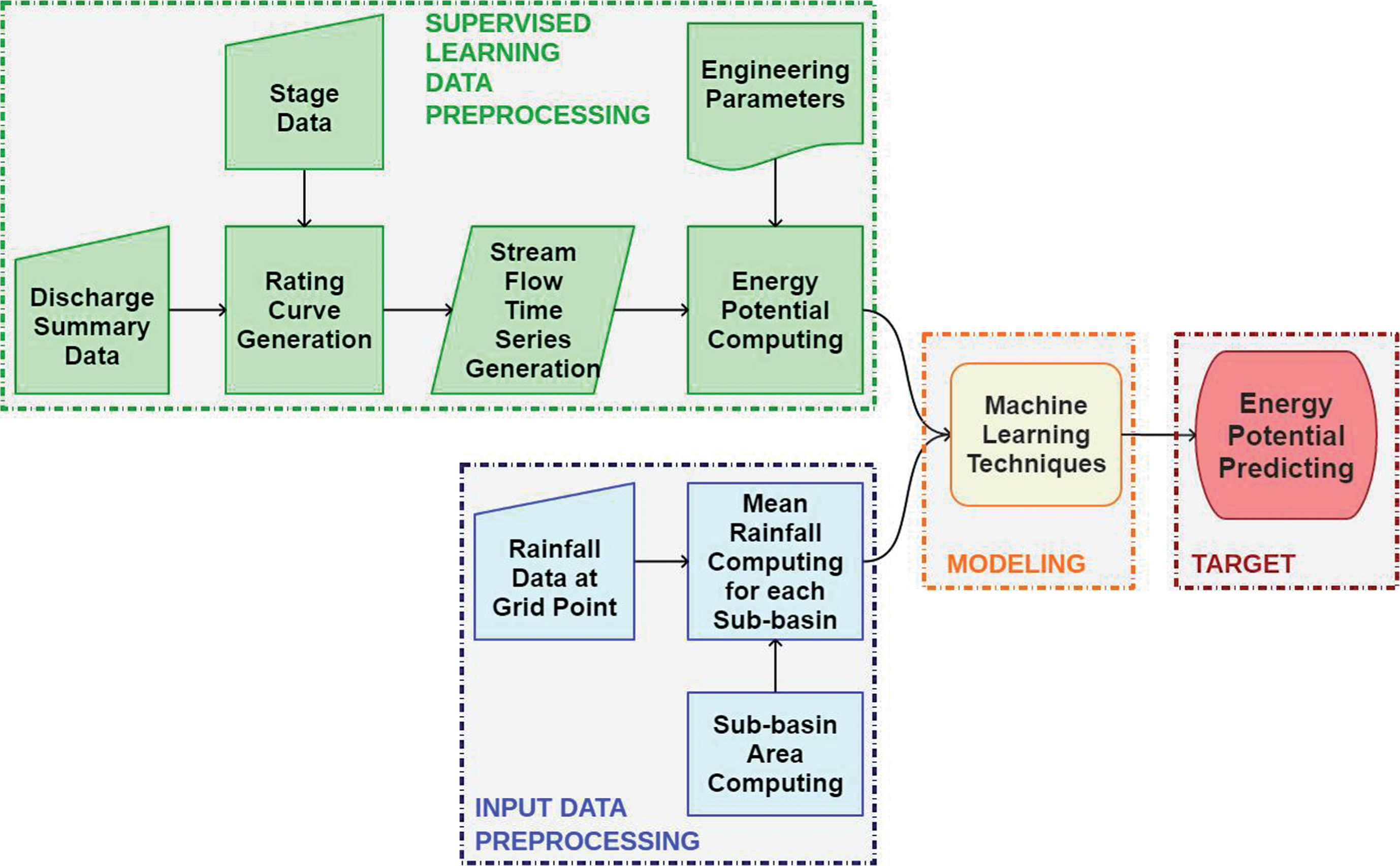
Process to forecasting the potential for energy generation.

Initially, summary discharge and stage data are processed to generate a rating curve that provides the stream flow time series. Stream flow dataset are converted into potential for hydropower generation by means of a mathematical equation that employs design parameters. The rainfall volumes in grid point are weighted for each sub-basin, generating a rainfall series per sub-basin. Finally, the rainfall data per sub-basin and the actual potential for hydropower generation are both introduced into a supervised network to modeling the potential for hydropower generation. The detailed description of each step of this process is presented following.

3.1 Discharge summary and stage dataset

At the measurement section of a river, stage gauge is used to measure the daily river height, i.e., the stage of the river. On the other hand, the discharge summary information consists of streamflow measurements taken during periodic field campaigns at a river section. The discharge measurements allow establishing a relation between stage and streamflow. This relationship is necessary for the systematic obtaining of the streamflow, no need of direct measurement. The stage-streamflow relationship is established graphically through the so-called discharge curve or rating curve of the section [44]. The rating curve is just an equation fitted to the streamflow measurement data (discharge summary).

3.2 Rainfall dataset

The rain has a strong relation with the streamflow and can be more easily obtained by both surface and orbital sensors. On the other hand, the rainfall presents large variability in time and space, which characterizes rainfall as a climatic variable of non-linear behavior. The precipitation information used in this research are available from the Climate Prediction Center / National Centers for Environmental Prediction (CPC / NCEP), whose dataset has global coverage in a 0.5° latitude ×0.5° longitude regular grid [45, 46]. This dataset is a combination of two kinds of data: a gauge-based (surface observations) analysis of daily precipitation and estimates of rainfall by satellites using the microwave and infrared channels. The period of coverage starts from January 1979 to the present day.

The daily rainfall data for each grid point was processed to obtain the mean monthly precipitation in each drainage area, i.e., the sub-basin of interest. The mean precipitation was determined using the methodology proposed by Thiessen [44, 47], as determined by the expression below: $\bar{P} = \frac{\sum_{i = 1}^{n} A_{i} P_{i}}{A}$ (11) where $\bar{P}$ is the mean precipitation at sub-basin; P_i is the precipitation at grid point; A is the sub-basin total area; and A_i is the grid point area belonging to the sub-basin.

3.3 Potential for hydropower generation

The potential for power generation of a hydropower plant is estimated using the following expression [5 , 48]: $P_{m} = η \times ρ \times Q_{m} \times g \times Δ h$ (12) where P_m is the mean monthly hydropower potential (in megawatts); η is the efficiency factor, which corresponds basically to the yield of the turbine-generator set; ρ is the water density (in kilograms per cubic meters); Q_m is the adjusted mean monthly discharge (in cubic meters per second); g is the gravitational acceleration (in meters per square second); Δh is the hydraulic head (in meters). The values for the variables are replaced in Equation (12) to generate the time series of monthly mean potential for energy generation, to calibrate and validate the model.

3.4 GMDH

The application of the GMDH method in this investigation considered the implementation of the multilayered iteration algorithm (MIA) with polynomial transfer functions. The MIA was considered appropriate for this research because it allows working with a large number of variables, which in turn requires the analysis of a large number of partial models combinations [49].

First, the partial models were compared based on bias, and then retrained based on total training and test data. The decision to cease training is adopted after comparing the relative error of the training layer with the minimum error of the layer. When that difference reaches a value lower than epsilon, then the training was terminated. The epsilon is the reference threshold of the training stop condition, whose value is 0.001.

The MIA can combine four types of polynomial transfer functions, as shown below: $- linear : y = w_{0} + w_{1} x_{1} + w_{2} x_{2}$ (13) $\begin{matrix} - linear - covariation : y = w_{0} + w_{1} x_{1} + w_{2} x_{2} + \\ + w_{3} x_{1} x_{2} \end{matrix}$ (14) $\begin{matrix} - quadratic : y = w_{0} + w_{1} x_{1}^{2} + w_{2} x_{2}^{2} + w_{3} x_{1} x_{2} + \\ + w_{4} x_{1} + w_{5} x_{2} \end{matrix}$ (15) $\begin{matrix} - cubic : y = w_{0} + w_{1} x_{1}^{3} + w_{2} x_{1}^{2} + w_{3} x_{1} + \\ + w_{4} x_{1}^{2} x_{2} + w_{5} x_{1} x_{2}^{2} + w_{6} x_{2}^{3} + w_{7} x_{2}^{2} + w_{8} x_{2} \end{matrix}$ (16)

The rainfall data for each single seven sub-basins are the input for the models. And they are lagged in up to twelve months, totaling up to 91 inputs. The dataset was separated into two independent samples. The first one, built with 33.33% to the training/validation set, i.e. 120 observations. And the second using the 66.66% remaining, i.e. 240 observations, which were used to test the model. The training/ validation dataset was divided into training and validation subsets as follows: training, validation, validation, validation, training, validation,..., training, validation, validation, validation, training, so that the last value is belonging to the training subset.

3.5 ANN

The neural network models with BPA were also designed using the same set of 91 input variables as previously described. The activation function adopted was the hyperbolic tangent. The architectures tested for the network showed that only one hidden layer was sufficient to model the potential for hydropower generation [50]. Two algorithms were tested for BPA optimization: Levenberg-Marquardt and Bayesian regulation. The tested configurations used from 1 to 90 neurons in the hidden layer, learning rates ranging from 0.01 to 0.5, momentum range from 0 to 0.9, and initial weight configurations were tested. To avoid overfitting the learning phase was interrupted in 100 iterations. The learning was stopped from the increase of the MSE. The learning data set was divided into training sample (80 observations) and validation sample (40 observations). The built models were validated based on the MSE of the validation set.

3.6 Model evaluation metrics

Evaluating the ability of the model is fundamental to define its application potential. For this, the following metrics are used to quantify the model performance: correlation coefficient (R), mean absolute error (MAE), and mean absolute percentage error (MAPE).

3.6.1 Correlation coefficient – R

The correlation coefficient (R) is a measure that indicates the association degree between two or more variables, whose interval of occurrence is limited between the – 1 and+1 values [51]. A correlation is considered weak when it reaches values below 0.6, obtained through the formulation below: $R = \frac{\sum_{i = 1}^{n} (x_{i} - \bar{x}) - (y_{i} - \bar{y})}{\sqrt{\sum_{i = 1}^{n} {(x_{i} - \bar{x})}^{2} {(y_{i} - \bar{y})}^{2}}}$ (17) where $x_{i} - \bar{x}$ is the deviation of each observation x_i from the mean of the response variable; $y_{i} - \bar{y}$ is the deviation of each observation y_i in relation to the mean of the predictor variable; and n is the number of observations.

3.6.2 Mean absolute error – MAE

The absolute mean error (MAE) consists of an arithmetic mean for the absolute values of the deviations between the members of each pair. This is a common measure to evaluate the accuracy of predictions for continuous predictors [52] and can be determined using the following equation: $MAE = \frac{1}{n} \sum_{i = 0}^{n - 1} | x_{i} - y_{i} |$ (18) where y_i is the estimated value of the ith observation; x_i is the corresponding real value; and n is the number of observations.

3.6.3 Mean absolute percentage error – MAPE

MAPE consists of a measure of error size in percentage terms and is used as an estimate of the accuracy of a forecast. $MAPE = \frac{100}{n} \sum_{i = 1}^{n} | \frac{x_{i} - y_{i}}{x_{i}} |$ (19) where the variables are similar as already described.

4 Case study

4.1 Site location

The proposed methodology for modeling the potential for hydropower generation was tested for the Jatobá HPP. The Tapajós River basin is in the Brazilian states of Pará, Mato Grosso, Amazonas and Rondônia, and belongs to the Amazon River basin. The Tapajós River has approximately 2,000 km long, is born in the Mato Grosso state, from the confluence of the Juruena and São Manuel Rivers, also known as Teles Pires, and flows into the Amazon River, already in the state of Pará [53]. The total area of the Tapajós river basin has 764,183 km², the relief ranging highlands to regions of hills and plateaus, whose altitude varying from 51 meters to about 900 meters [54]. The Tapajós River basin (Fig. 4) can be subdivided into seven smaller sub-basins, which have a drainage area that has a direct influence on the Jatobá HPP. The HPP Jatobá is situated approximately 1 km downstream from the town of Jatobá [54]:

Fig.4

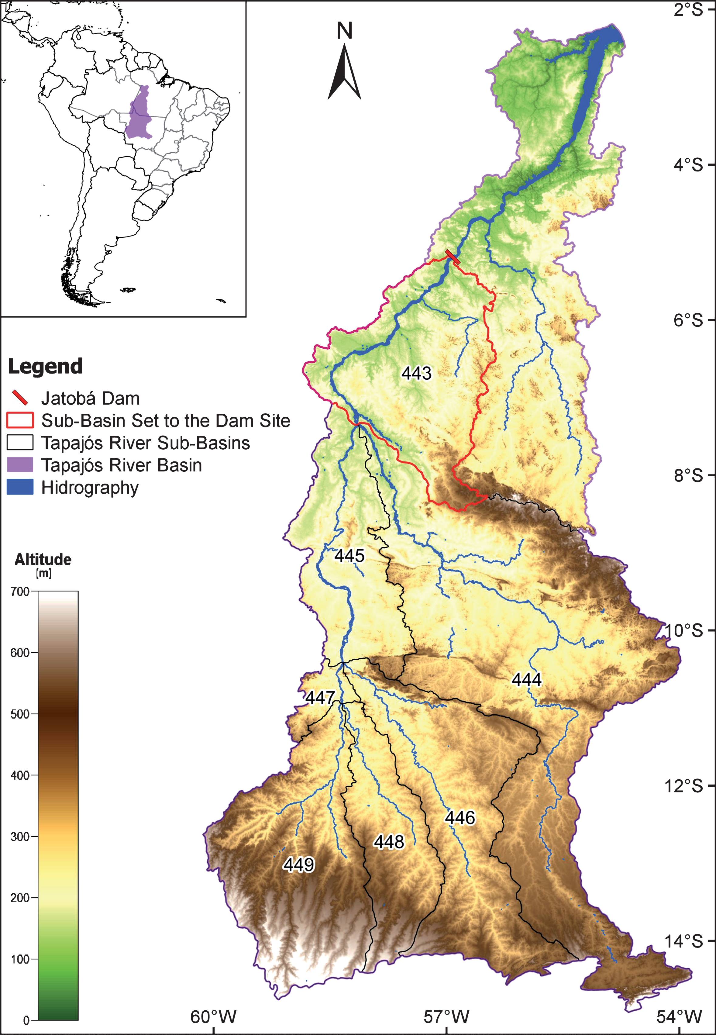
Tapajós River basin. The numerical codes presented in the delimited areas represent the sub-basins that compose the main basin of the Tapajós River. The sub-basins 443, 444, 445, 446, 447, 448 and 449 set the drainage area of the Jatobá HPP.

4.2 Data processing

This research used discharge summary data from Jatobá hydrological station (code 17650000), which is located at the municipality of Itaituba, Pará state. These data are made available by the National Water Agency (Agência Nacional de Águas - ANA) and cover the period from 1984 to1997.

The gauge height data comprise the period from 1984 up to the station decommissioning, which took place in 2013. Generally, ANA provides along with the discharge summary data, the rating curve for the river section. However, in this case, as there is no official rating curve published for the Jatobá station, it was necessary to develop an equation for the calculation of the stream flow series.

The determination of the rating curve (Fig. 5) to obtain the time series of flow at Jatobá it was executed by launching the discharge summary data in a calculation spreadsheet. Then, data fit functions were defined in polynomial form, exponential form, among others. The coefficient of determination (R²) was adopted as a criterion to select the best-fit function adapted to the river’s behavior, thus selecting a polynomial function of degree 2. Thus, using the rating curve and the monthly height gauge data, we can generate the time series of the monthly mean discharge at Jatobá. Then the discharge data are used in Equation (12) to determine the monthly potential for the hydropower generation, as will be detailed later.

Fig.5

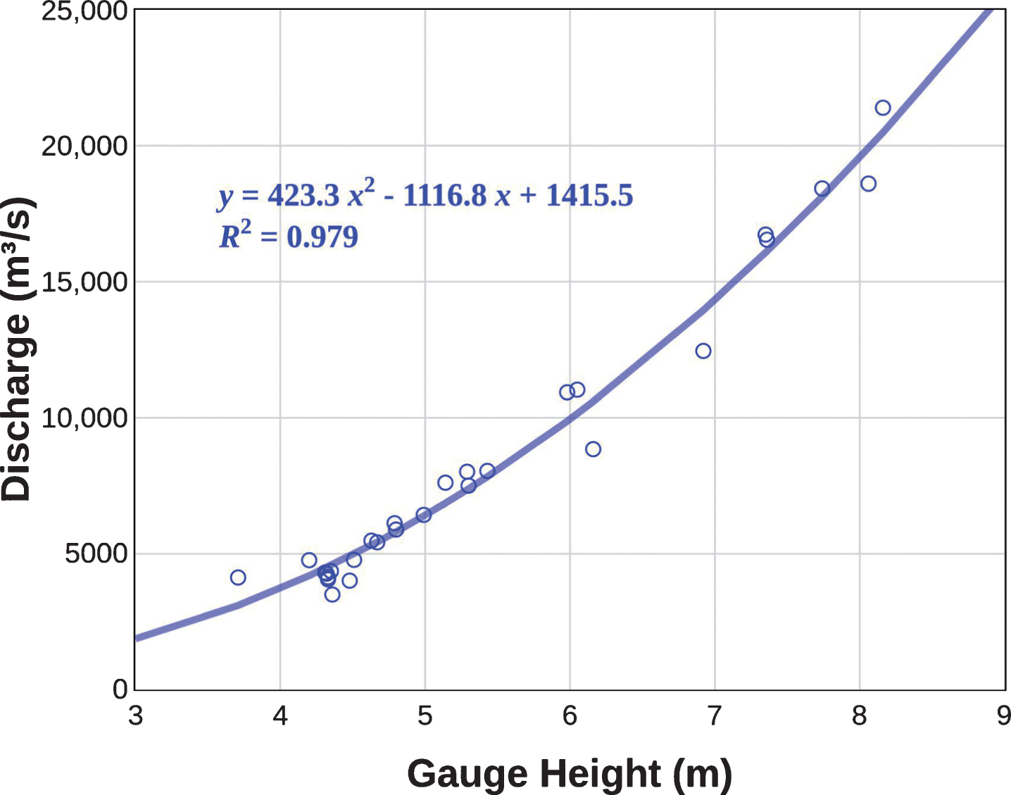
Rating curve to the Tapajós River at Jatobá gauge station.

The calculation of the river basin area and each grid point area (Fig. 6) was performed using the Quantum Gis geoprocessing software. Thus, the mean monthly rainfall time series was obtained for each the seven sub-basins of the Tapajós River that influence at Jatobá. This rainfall data are the input to the models to simulate the potential for hydropower generation. The sub-basin area 443 has been reduced from the original size and adjusted to the point where the dam will be installed. The new form adopted by sub-basin 443 considered the topography of the site and the drainage network, henceforth referred to as the Jat sub-basin (443 adjusted).

Fig.6

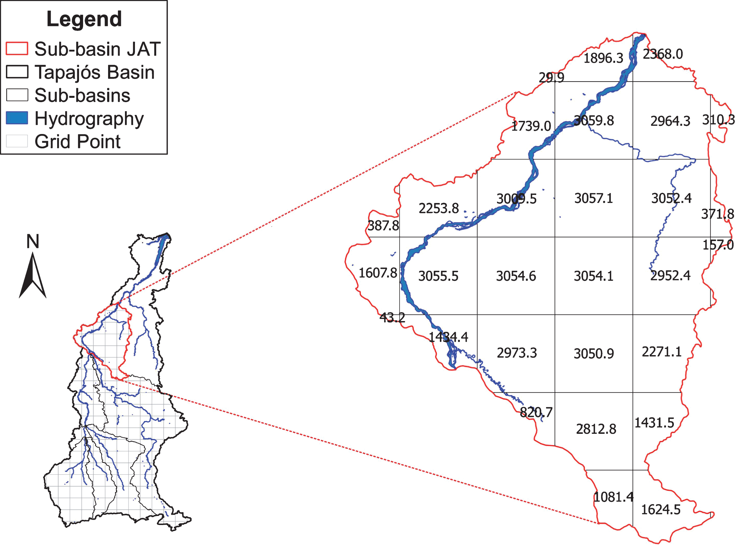
Area calculation for each grid point (in km²).

The specific engineering parameters are obtained from the design of the plant, as provided by the Energy Research Company (Empresa de Pesquisas Energéticas - EPE). They considered 35 meters for the hydraulic fall and 95% efficiency for the turbine-generator set. The values are replaced in Equation (12) for generate the time series of mean monthly potential for energy generation ranging the period from 1984 to 2013.

5 Results

To this paper several setups were tested for both GMDH and ANN. The best architecture obtained for the GMDH-type polynomial network selected 16 variables to build the model from 91 possible input variables, according to the following combinations: P-JAT₍₁₎, P-JAT₍₈₎, P-JAT₍₁₀₎, P-444, P-444₍₁₎, P-444₍₃₎, P-444₍₁₀₎, P-445, P-445₍₂₎, P-445₍₉₎, P-447, P-447₍₉₎, P-448₍₂₎, P-449, P-449₍₂₎, P-449₍₉₎, where the indices in parentheses show the time lag used. The activation functions employed were linear, linear covariance and quadratic. About the ANN models, the Levenberg-Marquardt algorithm, here called ANN-LM, had the best performance using 6 neurons in the hidden layer. While the ANN using Bayesian regulation algorithm, named as ANN-BR, obtained better results using 9 neurons in the hidden layer.

Table 1 shows the results of the models for the training and validation phases using some objective metrics of performance evaluation. Regarding the correlation (R) between the observed and simulation dataset, all the models showed good skill, with a slight advantage for the GMDH and ANN-BR, which reached 98% correlation. However, ANN-BR showed the lowest mean absolute error. By this criterion, the GMDH obtained inferior performance, although the difference between all the models was very small. On the other hand, the lowest percentage error (7.92%) was obtained by the GMDH, followed by ANN-BR (8.36%) and then ANN-LM (9.53%), respectively. Thus, the GMDH model obtained better performance for the R and MAPE criteria, while the ANN-BR model obtained the best performance for the R and MAE criteria. And the ANN-LM model showed worse performance for all evaluation criteria.

Table 1
Results for models’ evaluation (training/validation)

Metrics GMDH ANN-BR ANN-LM

R 0.98 0.98 0.97

MAE 265 245 251

MAPE (%) 7.92 8.36 9.53

Metrics	GMDH	ANN-BR	ANN-LM
R	0.98	0.98	0.97
MAE	265	245	251
MAPE (%)	7.92	8.36	9.53

In order to complement the understanding of Table 1, Fig. 7 presents a scatter plot. Regarding the distribution for the learning data (training and validation) around the best fit line, the ANN-BR model showed better correlation and lower dispersion in relation to the actual data, whose coefficient of determination was 0.9729.

Fig.7

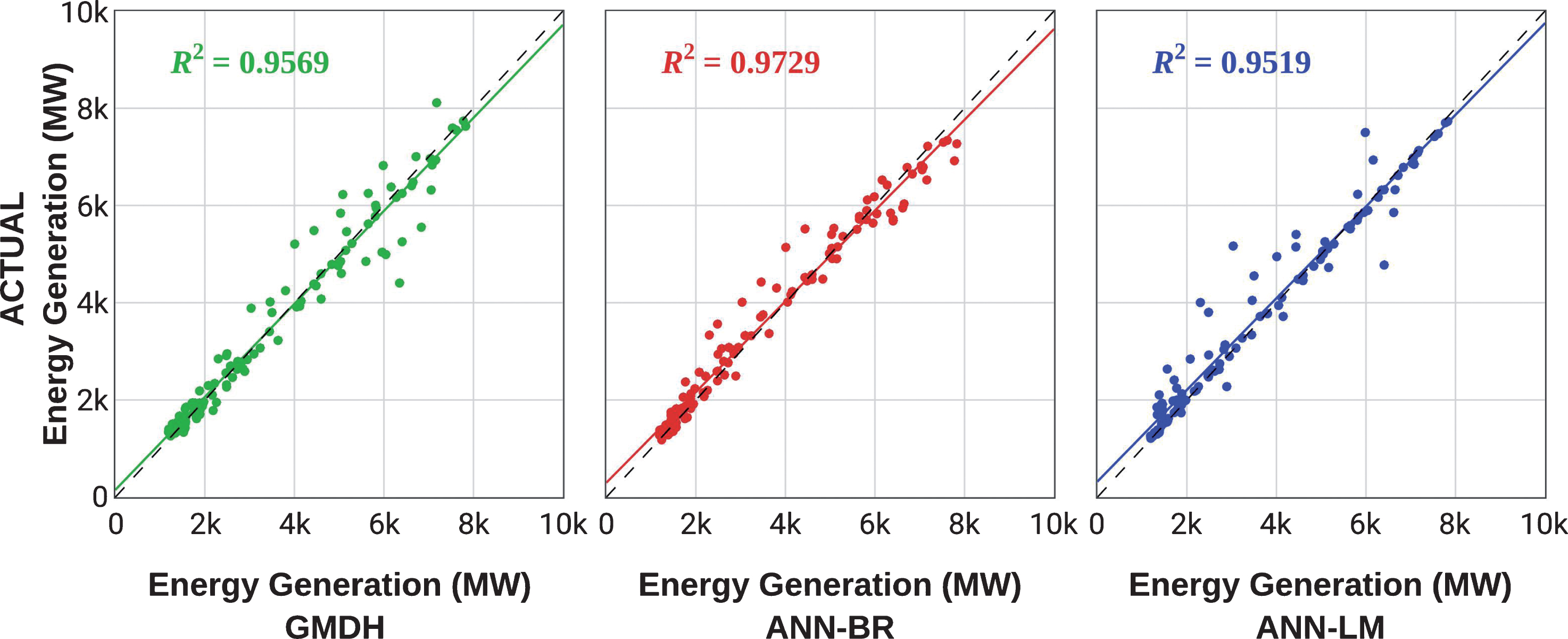
Agreement between the training/validation and actual data set.

The coefficient of determination consists of a measure about how much the independent variable(s) can explain the variation of the dependent variable. The models ANN-LM and GMDH also obtained good adjustments with the respective coefficients of determination, 0.9569 and 0.9519. However, the data simulated by these models showed greater dispersion. The dispersion of the data is not uniform along the different ranges of values, as will be discussed later.

The simulation for the learning dataset (training/validation) is shown in Fig. 8. In general, the models managed to good capture the seasonal behavior of the variable, showing great performance during the training phase. Although the extreme values of the series present large deviation, the found error is reduced, characterizing the good performance of the algorithms during the learning process.

Fig.8

Comparison between actual and training/validation values.

The ANN-LM model stands out for presenting an almost perfect fit for the training dataset (first 80 observations) and large variance for validation (last 40 observations), characterizing the difficulty for generalization of the model and overfitting tendency, with overestimation of the data. This behavior can be explained by the small number of observations for the training set and many variables (91) in the input layer. For such conditions, the smaller the number of neurons in the hidden layer, whatever the architecture adopted for the ANN-LM network, the number of parameters to be estimated will always be much higher than the number of observations. Many parameters against few observations for training reduce the network’s generalization ability by not capturing the complexities in the patterns between the input variables and the target, often leading to an overfitting [55]. This can explain the lower performance of the ANN-LM model compared to the others.

The performance of the ANN-BR model was similar throughout the learning phase, denoting better capacity for generalization. This behavior differs from the previous model because the regularization technique leads the biases of the parameters to the direction in which values are more probable. Therefore, this technique tends to reduce the variance of estimates in the cost of introducing biases [55].

Finally, the GMDH model also presented regular behavior throughout the training phase, being favored in this case by choosing the input variables of greater relevance for the modeling, optimizing the learning and avoiding the overfitting.

Figure 9 shows that the simulated data may have a greater or lesser dispersion depending on the range of simulation values. Thus, Fig. 9 presents a statistic that shows the limitation and distribution of model error for four different ranges of values: less than 2000, between 2000 and 4000, between 4000 and 6000, and greater than 6000. Since the relative error is strongly dependent on the actual data, it provides an idea of the forecast accuracy.

Fig.9

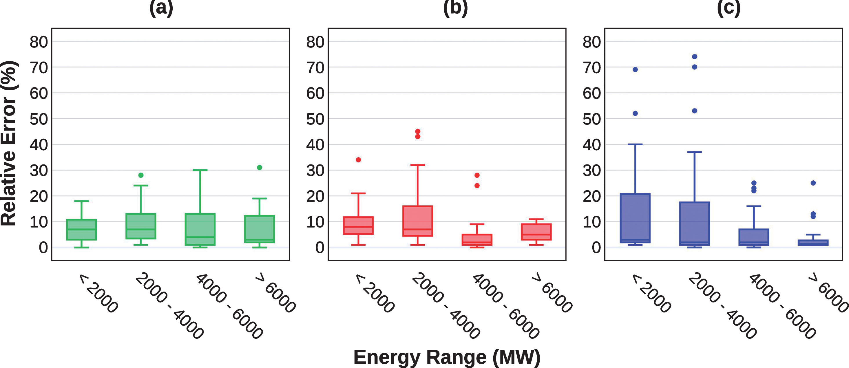
Relative error by energy band for the training/validation data set. (a) GMDH, (b) ANN-BR and (c) ANN-LM.

The first interval (<2000) is the most important for the forecast because it is associated with the minimum values, which should define the steady energy of the plant. Therefore, it is fundamental that the models present consistent behavior in this range. The GMDH model showed a symmetrical distribution for the relative error on the range less than 2000, centered in 7% (median) and with maximum 18%, and a small dispersion, all of them desirable conditions. For the second category (2000-4000) the error remained centered at 7%, but the dispersion was higher. In the following interval (4000-6000) the relative error distribution was quite asymmetric, with error reaching up to 30%. For the last interval that corresponds to the maximum values, there was an asymmetry increased and except for the outlier, the maximum relative error was below 20%.

Regarding the ANN-BR model, the error distribution was quite symmetrical for the lower interval, with error centered at 8% and outside reaching 21%, although one outlier occurred. For the following interval (2000-4000) there was marked asymmetry and large dispersion, with outside above 30%. On the range of values between 4000 and 6000, the ANN-BR showed its best performance, with a maximum error less than 10% and low dispersion, although two outliers were observed. And for the highest values, the relative error was around 5%, with low dispersion and variations of up to 11%.

The third model, ANN-LM, although it presented very small errors during the training, the validation phase clearly negatively influenced the overall performance of the model during the learning, making the error present large variation, especially in the first two classes of intervals, reaching up to 40% error. While in the last two interval classes, even with error reduction, especially for maximum values, many outliers still occurred.

Thus, during the learning phase, the GMDH model presented better accuracy for prediction values below 4000 MW, while the ANN-BR model obtained better accuracy for values above 4000 MW.

In relation to the test dataset, which is used to provide an unbiased evaluation of an adjusted final model, Table 2 presents the results of the accuracy of the developed models. The GMDH model presented the best performance compared to the others, although only slightly superior to ANN-BR. These indicators show that the GMDH model presented better capacity for generalization, because its performance during the test phase obtained a lower variation compared to the training phase, maintaining a good accuracy, with 0.95 correlation coefficient, 443 MW for the mean absolute error and only 12.34% mean percentage error.

Table 2

Results for models’ evaluation (test)

Metrics	GMDH	ANN-BR	ANN-LM
R	0.95	0.94	0.91
MAE	443	450	593
MAPE (%)	12.34	12.41	17.05

Figure 10 shows the adjustment curve between observation and prediction for the test dataset. ANN models presented lower capacity for generalization, with greater dispersion of the data and obtaining 0.88 and 0.83 coefficient of determination for the Bayesian regularization and Levenberg-Marquardt algorithm, respectively. The GMDH model reached the highest coefficient of determination, 0.90, meaning that the variables selected for the input layer can well explain the dependent variable and therefore the curve was fine fit on the scatter plot.

Fig.10

Agreement between the test and actual data set.

The models’ skill can best be seen in Fig. 11, which refers to the test subset. In general, the models’ performed a good skill, highlighting the excellent simulation for the minimum values, specially to GMDH and ANN-BR. Clearly, there were underestimates of the peaks occurred for the year 2005 up to 2009, and from 2012 to 2013. Probably this behavior is associated with the dataset of the CPC. In general, for regions with poor rainfall coverage, and it happens in Amazon region, the grid point data of the CPC tend to underestimate the severe events with too voluminous rainfall due to convective precipitation [56]. Therefore, it is very likely that a noisy input data has led to larger errors during the simulation of the energy maximum peak. However, the possible underestimate of the peaks, while not desirable, does not compromise the feasibility studies of the project which is based on the critical point.

Fig.11

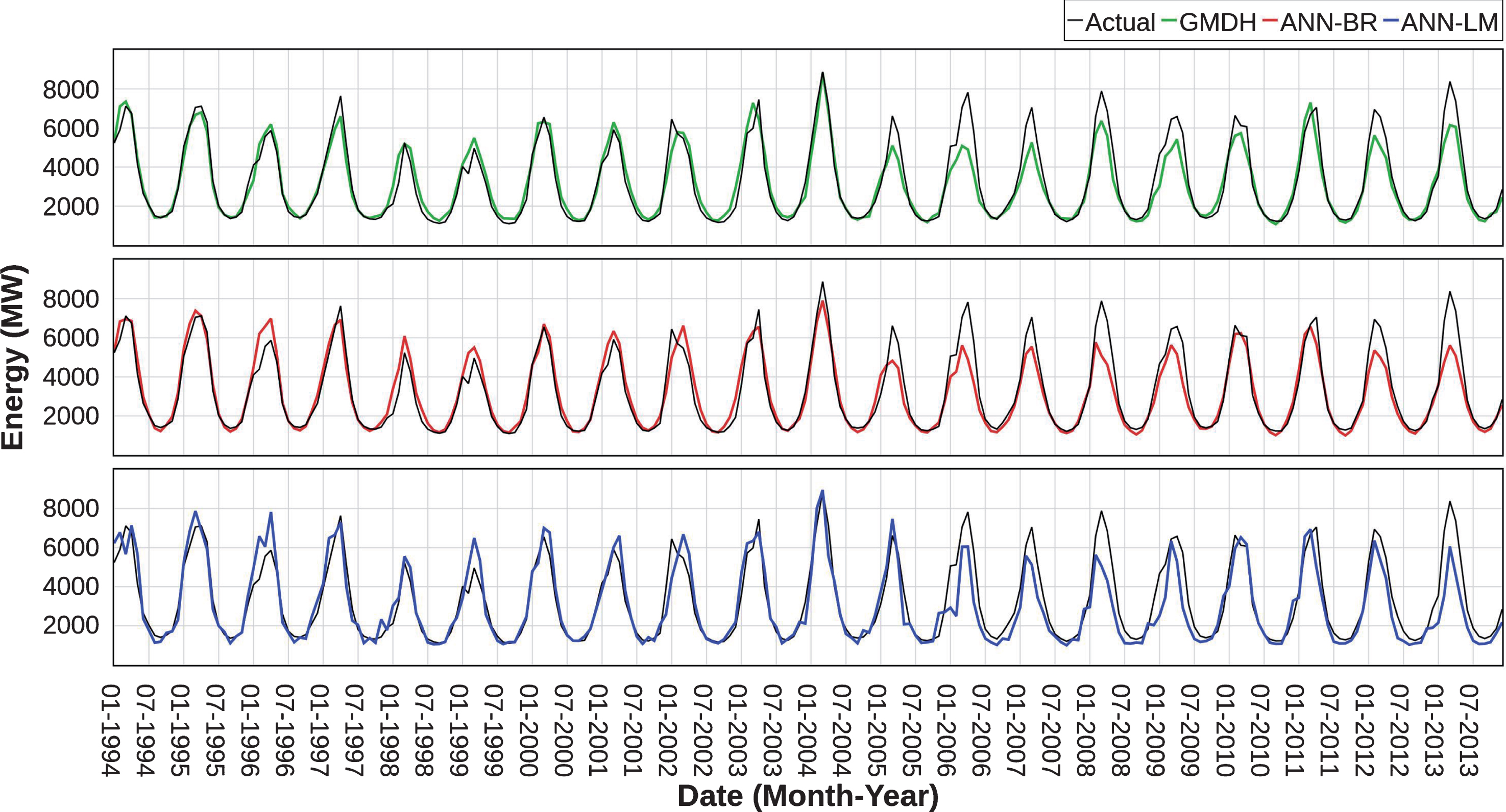
Comparison between actual and testing values.

Such as the learning phase, during the test period the error of the models was higher for the higher values of power generation but presented low values for the minimums. For the precursor studies that define the potential for the power generation of a hydroelectric plant, especially those of the run-of-the-river type, it is fundamental to determine the critical points of lower natural flow from the historical data, which correspond to the lower generation of energy and should define the steady energy of the plant, i.e., the maximum continuous production of energy.

From the test dataset, Fig. 12 shows the variation of the relative error by range of values. For the lower range, the GMDH model presented better performance than the others, with an average error around 8%, but very close to the ANN-BR model. In relation to the following classes, the mean error varied between 11% and 17% for the GMDH model, while the ANN-BR model showed a constant average error around 12%, but with greater variability, even with some outliers. In the second and third categories of values there was alternation of better performance between ANN-BR and GMDH. While in the latter category both the models, GMDH and ANN-BR, achieved very similar performance. The ANN-LM model presented lower behavior, with a large interquartile range and the worst performance comparing to all classes of values.

Fig.12

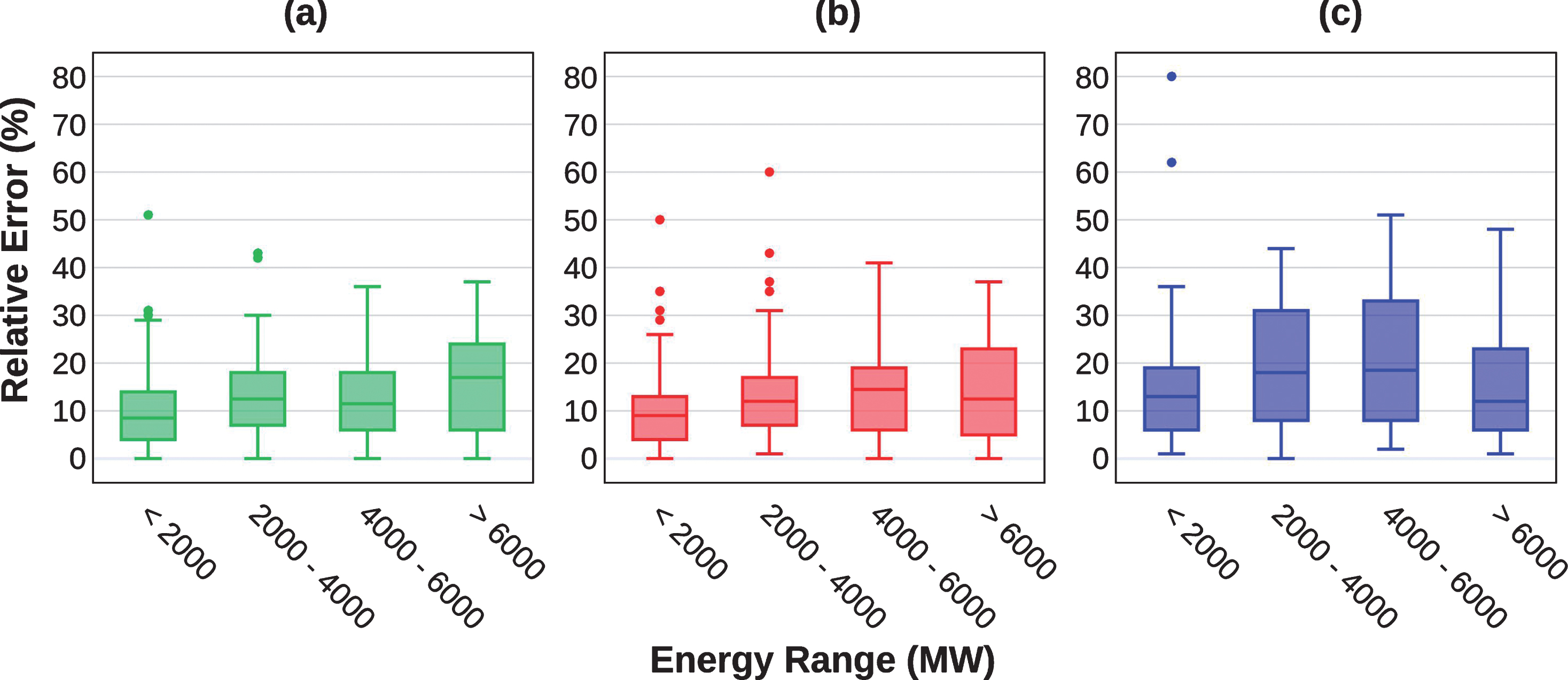
Relative error by energy band for the test data set. (a) GMDH, (b) ANN-BR and (c) ANN-LM.

The coefficients of determination and correlation indicated a strong relation between the chosen independent variables (monthly mean precipitation) and the dependent variable. This allowed us to model the potential for hydropower generation to achieve high dexterity. About the simulation error, both learning and forecast results obtained satisfactory error rate.

6 Conclusion

The machine learning approach proved to be a successful and robust tool able to model with high dexterity the power generation of a hydroelectric enterprise in the Amazon, from the rainfall regime.

The modeling of the potential for hydropower generation was studied using the GMDH and ANN techniques. The three GMDH, ANN-BR and ANN-LM algorithms were used to build the polynomial and MLP neural network architectures. The prediction of energy potential, especially for the critical period of generation, performed better with the GMDH approach, although Bayesian regularization achieved quite close performance.

The ANN-LM showed to be inadequate for the studied purpose, presenting low ability for generalization and, therefore, large dispersion of data and less accuracy.

The self-organizing feature of the GMDH network showed to be very appropriate for selecting the best-input arguments of the network to optimize the model result. The performance of the GMDH network showed a good skill, especially to safely capture the critical points.

Finally, this methodology ensuring statistical safety in its results, which will allow a better prior evaluation of the energy potential predicting by the project. It can improve the planning of scenarios, especially those related to the natural variability of the rainfall behavior. It can reduce the operational costs, especially those associated to the field activities for flow measurements and maintenance of hydrometric stations. In addition, it can generate synthetic time series of the potential for energy generation, covering periods without local observation of the stream flow, allowing to extend the historical data to assist in the preliminary and sequential studies of the plant.

References

EPE. Brazilian Energy Balance 2017 Year 2016. 2017.

Fearnside

P.M.

, Dams in the Amazon: Belo Monte and Brazil’s hydroelectric development of the Xingu River Basin, Environ Manage 38 (2006), 16–27. doi:10.1007/s00267-005-0113-6 .

Fearnside

P.M.

, Impacts of Brazil’s Madeira River Dams: Unlearned lessons for hydroelectric development in Amazonia, Environ Sci Policy 38 (2014), 164–72. doi:10.1016/j.envsci.2013.11.004 .

Brazil

M.M.E.

, (Ministry of Mines and Energy). Manual for hydropower inventory studies of river basins. 2007 Ed. Rio de Janeiro: Brazil MME. 2007.

Sharma

, Singh

, Run off river plant: status and prospects, Int J Innov Technol Explor Eng 3 (2013), 210–3.

Tolmasquim

M.T.

, Energia renovável: hidráulica, biomassa, eólica, solar, oceânica. Rio de Janeiro: EPE (Energy Research Company), 2016.

Koch

, Prasch

, Bach

, Mauser

, Appel

, Weber

, How will hydroelectric power generation develop under climate change scenarios? A case study in the upper danube basin, Energies 4 (2011), 1508–41. doi:10.3390/en4101508 .

IRENA (International Renewable Energy Agency). Hydropower Technology Brief. Abu Dhabi, 2015.

Stickler

C.M.

, Coe

M.T.

, Costa

M.H.

, Nepstad

D.C.

, McGrath

D.G.

, Dias

L.C.P.

, et al. Dependence of hydropower energy generation on forests in the Amazon Basin at local and regional scales, Proc Natl Acad Sci 110 (2013), 9601–6. doi:10.1073/pnas.1215331110 .

10.

Wali

U.G.

, Estimating Hydropower Potential of an Ungauged Stream, Int J Emerg Technol Adv Eng 3 (2013), 592–600.

11.

ANEEL (Agência Nacional de Energia Elétrica). Atlas de energia elétrica do Brasil. Brasília, 2002.

12.

ANEEL (Agência Nacional de Energia Elétrica). Cadernos Temáticos ANEEL 3 – Energia Assegurada. Brasília, 2005.

13.

Awojobi

, Jenkins

G.P.

, Managing the cost overrun risks of hydroelectric dams: An application of reference class forecasting techniques. Renew Sustain Energy Rev, 2016. doi:10.1016/j.rser.2016.05.006 .

14.

Cheng

C-H.

, and YangJun-He , A novel rainfall forecast model based on the integrated non-linear attribute selection method and support vector regression, J Intell Fuzzy Syst 31 (2016), 915–25. doi:10.3233/JIFS-169021 .

15.

Ahmad

A.S.

, Hassan

M.Y.

, Abdullah

M.P.

, Rahman

H.A.

, Hussin

, Abdullah

, et al. A review on applications of ANN and SVM for building electrical energy consumption forecasting, Renew Sustain Energy Rev 33 (2014), 102–9. doi:10.1016/j.rser.2014.01.069 .

16.

Elattar

E.E.

, Goulermas

J.Y.

, Wu

Q.H.

, Generalized locally weighted GMDH for short term load forecasting, IEEE Trans Syst Man Cybern Part C Appl Rev 42 (2012), 345–56. doi:10.1109/TSMCC.2011.2109378 .

17.

Abdel-Aal

R.E.

, Improving electric load forecasts using network committees, Electr Power Syst Res 74 (2005), 83–94. doi:10.1016/j.epsr.2004.09.007 .

18.

Abdel-Aal

R.E.

, Modeling and forecasting electric daily peak loads using abductive networks, Int J Electr Power Energy Syst 28 (2006), 133–41. doi:10.1016/j.ijepes.2005.11.006 .

19.

Zjavka

, Snáşel

, Short-term power load forecasting with ordinary differential equation substitutions of polynomial networks, Electr Power Syst Res 137 (2016), 113–23. doi:10.1016/j.epsr.2016.04.003 .

20.

Srinivasan

, Energy demand prediction using GMDH networks, Neurocomputing 72 (2008), 625–9. doi:10.1016/j.neucom.2008.08.006 .

21.

Xiao

, Sun

, Hu

, Xiao

, GMDH based auto-regressive model for China’s energy consumptionprediction, Int. Conf. Logist. Informatics Serv. Sci. LISS, (2015), 2015. doi:10.1109/LISS.2015.7369754 .

22.

Witczak

, Korbicz

, Mrugalski

, Patton

R.J.

, A GMDH neural network-based approach to robust fault diagnosis: Application to the DAMADICS benchmark problem, Control Eng Pract, 14 (2006), 671–83. doi:10.1016/j.conengprac.2005.04.007 .

23.

, Upadhyaya

B.R.

, Coffey

L.A.

, Model-based monitoring and fault diagnosis of fossil power plant process units using Group Method of Data Handling, ISA Trans 48 (2009), 213–9. doi: S0019-0578(08)00075-X [pii] 10.1016/j.isatra.2008.10.014 .

24.

Ikeda

, Sawaragi

, Ochiai

, Sequential GMDH algorithm and its application to river flow prediction, IEEE Trans Syst Man Cybern 6 (1976), 473–9. doi:10.1109/TSMC.1976.4309532 .

25.

Ivakhnenko

A.G.

, The group method of data handling – a rival of the method of stochastic approximation, Sov Autom Control c/c Avtom 1 (1968), 43–55.

26.

Farlow

S.J.

, Self-Organizing Methods in Modelling: GMDH Type Algorithms. New York: Marcel Dekker, 1984.

27.

Farlow

S.J.

, The gmdh algorithm of ivakhnenko, Am Stat 35 (1981), 210–5. doi:10.1080/00031305.1981.10479358 .

28.

Ivakhnenko

A.G.

, Ivakhnenko

G.A.

, The review of problems solvable by algorithms of the group method of data handling (GMDH), Pattern Recognit Image Anal C/C Raspoznavaniye Obraz I Anal Izobr 5 (1995), 527–35.

29.

Mrugalski

, An unscented kalman filter in designing dynamic gmdh neural networks for robust fault detection, Int J Appl Math Comput Sci 23 (2013), 157–69. doi:10.2478/amcs-2013-0013 .

30.

Dag

, Yozgatligil

, GMDH: An R Package for Short Term Forecasting via GMDH – Type Neural Network Algorithms. R J, XX (2012), 1–8.

31.

Ivakhnenko

A.G.

, Polynomial theory of complex systems, IEEE Trans Syst Man Cybern 1 (1971), 364–78. doi:10.1109/TSMC.1971.4308320 .

32.

, Dong

, Wu

, Zhao

, Application of GMDH to short-term load forecasting. Adv. Intell. Soft Comput., AISC, 138 (2012), 27–32. doi:10.1007/978-3-642-27869-3_4 .

33.

Neural

Haykin.

, Networks and Learning Machines, 2009.

34.

Doan

C.D.

, Liong

, Generalization for multilayer neural network: Bayesian regularization or early stopping. 2nd Asia Pacific Assoc. Hydrol. Water Resour., Suntec - Singapore, 2004, pp. 5–8.

35.

Rumelhart

D.E.

, Hinton

G.E.

, Williams

R.J.

, Learning representations by back-propagating errors, Nature 323 (1986), 533–6. doi:10.1038/323533a0 .

36.

Jani

D.B.

, Mishra

, Sahoo

P.K.

, Application of artificial neural network for predicting performance of solid desiccant cooling systems – A review, Renew Sustain Energy Rev 2017. doi:10.1016/j.rser.2017.05.169 .

37.

Hinton

G.E.

, Osindero

, The

Y-W.

, A fast learning algorithm for deep belief nets, Neural Comput 18 (2006), 1527–54. doi:10.1162/neco.2006.18.7.1527 .

38.

Xie

, Zhang

, Singh

, Reliability forecasting models for electrical distribution systems consideringcomponent failures and planned outages, Int J Electr Power Energy Syst, 2016. doi:10.1016/j.ijepes.2016.01.020 .

39.

Hagan

M.T.

, Menhaj

M.B.

, Training Feedforward Networks with the Marquardt Algorithm, IEEE Trans Neural Networks 5 (1994), 989–93. doi:10.1109/72.329697 .

40.

Demuth

H.B.

, Raele

M.H.

, Neural Network Toolbox User’s Guide for use with Matlab, 2009.

41.

MacKay

D.J.C.

, Bayesian interpolation, Neural Comput 4 (1992), 415–47. doi:10.1162/neco.1992.4.3.415 .

42.

Saini

L.M.

, Peak load forecasting using Bayesian regularization, Resilient and adaptive backpropagation learning based artificial neural networks, Electr Power Syst Res, 2008. doi:10.1016/j.epsr.2007.11.003 .

43.

Foresee

F.D.

, Hagan

M.T.

, Guass-Newton approximation to bayesian learning, Proc. Int. Conf. Neural Networks, Houston, Texas, 1997, pp. 1930–5.

44.

Raghunath

H.M.

, Hydrology – principles, analysis, design. 2nd Ed. New Delhi: New Age, 2006.

45.

Xie

, Chen

, Yang

, Yatagai

, Hayasaka

, Fukushima

, et al. A Gauge-Based Analysis of Daily Precipitation over East Asia, J Hydrometeorol 2007. doi:10.1175/JHM583.1 .

46.

Chen

, Shi

, Xie

, Silva

V.B.S.

, Kousky

V.E.

, Higgins

R.W.

, et al. Assessing objective techniques for gauge-based analyses of global daily precipitation, J Geophys Res Atmos 113 (2008). doi:10.1029/2007JD009132 .

47.

Thiessen

, Precipitation averages for large areas, Mon Weather Rev 39 (1911), 1082–9.

48.

Butera

, Balestra

, Estimation of the hydropower potential of irrigation networks, Renew Sustain Energy Rev, 2015. doi:10.1016/j.rser.2015.03.046 .

49.

Kordík

, GAME – Hybrid self-organizing modeling system based on GMDH, Stud Comput Intell 211 (2009), 233–80. doi:10.1007/978-3-642-01530-4_6 .

50.

Basheer

I.A.

, Selection of methodology for neural network modeling of constitutive hystereses behavior of soils, Comput Civ Infrastruct Eng, 2000. doi:10.1111/0885-9507.00206 .

51.

Chartterjee

, Hadi

A.S.

, Regression Analysis by Example. 5th ed. New Jersey: John Wiley & Sons Inc, 2012.

52.

Wilks

D.S.

, Statistical Methods in the Atmospheric Sciences, 2nd Ed. New York: Academic Press, 2006.

53.

Sousa

, Júnior, Tapajós: hidrelétricas, infraestrutura e caos. Elementos para a governança em uma região singular. 1st Ed. São José Dos Campos: ITA/CTA, 2014.

54.

ELETRONORTE, Camargo Correa, CNEC. Estudos de Inventário Hidrelétrico das Bacias dos Rios Tapajós e Jamanxim. Rio de Janeiro: 2008.

55.

Okut

, Bayesian Regularized Neural Networks for Small n Big p Data. Artif. Neural Networks, INTECH, 2016, pp. 27–48. doi:10.5772/63256 .

56.

Beck

H.E.

, Vergopolan

, Pan

, Levizzani

, Van Dijk

A.I.J.M.

and Weedon

G.P.

, et al. Global-scale evaluation of 22 precipitation datasets using gauge observations and hydrological modeling, Hydrol Earth Syst Sci, 2017. doi:10.5194/hess-21-6201-2017 .

Artificial neural networks approaches for predicting the potential for hydropower generation: a case study for Amazon region

Abstract

Keywords

1 Introduction

2 Machine Learning and Related Works

2.1 Group method of data handling (GMDH)

3.2 Rainfall dataset

3.6 Model evaluation metrics

3.6.1 Correlation coefficient – R

4.1 Site location

Table 1 Results for models’ evaluation (training/validation) Metrics GMDH ANN-BR ANN-LM R 0.98 0.98 0.97 MAE 265 245 251 MAPE (%) 7.92 8.36 9.53

References

Table 1
Results for models’ evaluation (training/validation)

Metrics GMDH ANN-BR ANN-LM

R 0.98 0.98 0.97

MAE 265 245 251

MAPE (%) 7.92 8.36 9.53