Efficient methods to set decay factor of time decay model over data streams

2.1. Preliminaries

A data stream DS =< T₁, T₂, …, T _i , … > is a continuous and unbounded sequence of transactions, where T _i  (i = 1, 2, …) is the ith transaction. Let A = {a₁, a₂, …, a _n } be a set of items in DS, and T _i  (i = 1, 2, …) is a subset of A. A transaction is a tuple, denoted as (TID, itemset), contains a unique transaction identifier TID and an itemset, as shown in Table 1.

In the applications of time-sensitive data stream, users are most interested in the recently arrived transactions, thus the sliding window model is suitable for such cases. A sliding window SW of size N contains the nearly N transactions in DS. A frequent pattern P = {p₁, p₂, …, p _k } is also a subset of A. The frequency of P, denoted as freq (P), is the number of transactions in SW where P occurs. The support of P in SW, denoted as sup(P), is defined as freq (P)/N. P is a frequent pattern in SW if sup(P) ≥ θ, where θ (0 ≤ θ ≤ 1) is a minimum support threshold. P is a frequent closed pattern in SW, if P is a frequent itemset in SW and there exists no itemset Y in SW such that X ⊂ Y and freq (X) = freq (Y). In this paper, we will focus on mining frequent closed pattern over data stream on the basis of sliding window model and time decay model.

Due to the continuity and infinite, the knowledge contained in data stream may change over time. Under normal circumstances, the value of the recent transaction is more important than the historical one. Therefore, it is necessary to increase the weight of recent transaction. A TDM is developed to decay gradually the occurrence frequency of the patterns contained in the transactions with time [5].

Let the decay ratio of frequency in the unit time is decay factor f  (f ∈ (0, 1]). When transaction T _i arrives, the decay frequency of a pattern P is denoted as freq_d  (P, T _i ). When T arrives, freq_d (P, T) is initialized to be 1 if it contains P, and 0 otherwise. Each time a new transaction arrives, freq_d (P, T) is multiplied by a decay factor f. As the new transaction T _m arrives, the decay frequency freq_d (P, T _m ) of P is calculated by Formulas 1 and 2. When the mth transaction T _m arrives, r is 1 if it contains P, otherwise r = 0.

freq d ( P , T m ) = { r , if m = 1 freq d ( P , T m - 1 ) × f + r , if m ≥ 2(1) r = { 1 , if P ⊆ T m 0 , else(2)

From the above formulae, it can be concluded that the decay frequency of pattern P is smaller than its original frequency, that is freq_d (P) ≤ freq (P). For instance, set sliding window size N = 1000 and minimum support threshold θ = 0.01. If freq (P) ≥ θ × N = 10, P is a frequent pattern. However, let the decay factor f = 0.8, then freq_d (P) <1/(1 - 0.8) =5 as calculated by Formula 3. That means no pattern can be mined out under the time decay model. freq d ( P , T m ) = freq d ( P , T m - 1 ) × f + r = ∑ i r i × f m - i = r 1 × f m - 1 + r 2 × f m - 2 + … + r m ≤ f m - 1 + f m - 2 + … + 1 ≤ 1 1 - f(3)

With TDM, some possible frequent patterns may be lost with only minimum support threshold. In order to reduce the number of missing possible patterns, frequent patterns and sub-frequent patterns need to be maintained during mining process. In addition, in order to reduce the cost of maintaining patterns, non-frequent patterns need to be abandoned. The definitions of frequent patterns are shown as follows. By this method, the possible error of lost patterns is no greater than the maximal support error ɛ [5].

Definition 1. Let θ (θ ∈ (0.1]) be the minimum support and ɛ (ɛ ∈ (0, θ)) be the maximal support error. If freq_d (P) ≥ θ × N, P is a frequent pattern. If ɛ × N ≤ freq_d (P) < θ × N, P is sub-frequent pattern. Otherwise, if freq_d (P) < ɛ × N, P is non-frequent pattern.

Example 1. There are 4 transactions in data stream as shown in Table 1. Let minimum support θ = 0.5, maximal support error ɛ = 0.1 × θ and decay factor f = 0.8. Using Formula 1 to generate decay frequency, the mining process on data stream is shown in Fig. 1. ClosedTable, which consists of three fields: Cid, CP and SCP, that is used to maintain the information of closed itemsets. Each closed itemset CP is assigned a unique closed identifier Cid, and its decay frequency is denoted as SCP. When a new transaction T _m arrives, the frequencies of all itemsets in ClosedTable are needed to be updated. The details are shown in FrequentTable in Fig. 1. For instance, when T _m arrives, we update ClosedTable first. Works include updates: freq_d = ({1 3 4}) =0.8 × f + r⁽³⁾ = 0.64,  r⁽³⁾ = 0; freq_d = ({2 3 5}) =1 × f + r⁽³⁾ = 1.8, freq_d = ({3}) =1.8 × f + r⁽³⁾ = 2.44, and r⁽³⁾ = 1. Next step is adding a new itemset {1 2 3 5} into ClosedTable, and freq_d = ({1 2 3 5}) = r⁽³⁾ = 1. So repeatedly, all frequencies of itemsets are generated.

OPEN IN VIEWER

Fig.1

Mining frequent patterns on data stream based on TDM.

A decay function takes the initial weight and the age of an itemset. Therefore, the weight of an itemset in the sketch can decrease with time according to a user-specified decay function.

Definition 2. A decay function factor (f,  x) takes two parameters, the decay factor f ≥ 0 and an integral age x ≥ 0, which should satisfy the following conditions. (1) factor (f,  x) ≥0 for all f, x; (2) if f₁ > f₂, then factor (f₁, x) ≥ factor (f₂, x); (3) if x₁ > x₂, then factor (f,  x₁) ≤ factor (f,  x₂).

Recently, the commonly used decay function is like factor (f,  x) = f ^x , where x is the age, and f is the decay factor. There are three types of values to set the decay factor f: user-specified value, constant value and variable value.

(1) Set the decay factor to a user-specified value in the range of (0, 1].

For instance, algorithm IncSpam [16] performs the mining of sequential patterns over a sliding window by using a lexicographical tree. And it reflects the greater importance of more recent information by means of a static decay function with a user-defined decay value of 0.999. Framework GUIDE [17] mines maximal high utility itemsets from data streams by assuming the decay factor as 0.9. DUF-streaming [14] uses the time fading window to mine frequent itemsets from uncertain data streams with setting time fading f to a user-specified value in the range of (0,1]. MPM [26] defines a damping factor, which is a real number ranging from 0 to 1. Then, the importance of transactions generated from data streams is determined by this factor. If time passes after a transaction arrives from a data stream, the importance of the transaction (frequency, utility, etc.) is multiplied by the factor.

Setting the decay factor to a user-specified value may lead to different function values. For example, let f = 0.9999, 0.999, 0.99 or 0.9 and x = 1, 100 and 1000, then the values of factor (f,  x) are very different as shown in Table 2. If f = 0.999 (as in algorithm IncSpam [16]) and x = 1000, then factor (f,  x) =0.90483289. While if f = 0.9 (as in GUIDE [17]) and x = 1000, then factor (f,  x) =1.7479E - 46. The gap of these two decay function values is large. Therefore, setting f to user-specified values may cause unstable mining results.

(2) Set the decay factor to a constant value regardless of parameter N.

Chang [3] and Lee [13] define a decay factor by two parameters: a decay-base b and a decay-base-life h. A decay-base b determines the amount of weight reduction per a decay-unit and it is greater than 1. When the weight of the current information is set to 1, a decay-base-life h is defined by the number of decay-units that makes the current weight be b^-1. Based on these two parameters, a decay factor f _d is defined as shown in Formula 4 where b > 1,  h ≥ 1,  b^-1 ≤ f _d  < 1. f d = b - ( 1 h )(4)

HewaNadungodage [11] suggested that the half-life should be used to set the decay factor so as to mine frequent patterns over uncertain data streams. Half-life, which is denoted by t_1/2, is the period of time which takes for a substance undergoing decay to be decreased by half. An exponential decay process can be described by the following Formula: f = e - α(5) where α is a positive number called the decay constant of the decaying quantity and its value is: α = ln 2 t 1 / 2 .

And the value of decay factor is shown as Formula 6.

f _ halflife = e - ( ln 2 t 1 / 2 )(6)

These methods set the decay factor f without considering its relationship with the sliding window size. Therefore, with the change of the window size, the performance of algorithm may be quite different.

(3) Set the decay factor to variable value related to parameters N, θ and ɛ.

Some of the frequent patterns retrieved by stream mining algorithm are sub-frequent or non-frequent. To measure the quality of approximate mining results, two performance metrics recall and precision [5, 6] are commonly used. Given a set of true frequent patterns Q and a set of retrieved patterns O, then recall = | Q ∩ O | | Q | , precision = | Q ∩ O | | O | .(7)

Two conditions are used to set the decay factor. Firstly, assuming recall of the algorithm is 100%, all frequent patterns are discovered under the time decay model. Consider a situation in which only θ × N transactions contain the pattern P, then P is frequent for freq (p) ≥ θN. In order to get 100% recall, P should be selected even though the decayed frequency of P reaches its minimum. Theorem 1 shows a lower bound for the decay factor if 100% recall is assumed.

Theorem 1. With the time decay model, recall will be 100% if the decay factor f satisfies the following condition: f ≥ ( 2 N - θ N - 1 ) [ ( θ - ɛ ) / θ ] 2(8)

Proof. Suppose θN transactions contain P which are the oldest transactions in SW, as shown in Fig. 2(a). Thus the minimum decay frequency of P is:

OPEN IN VIEWER

Fig.2

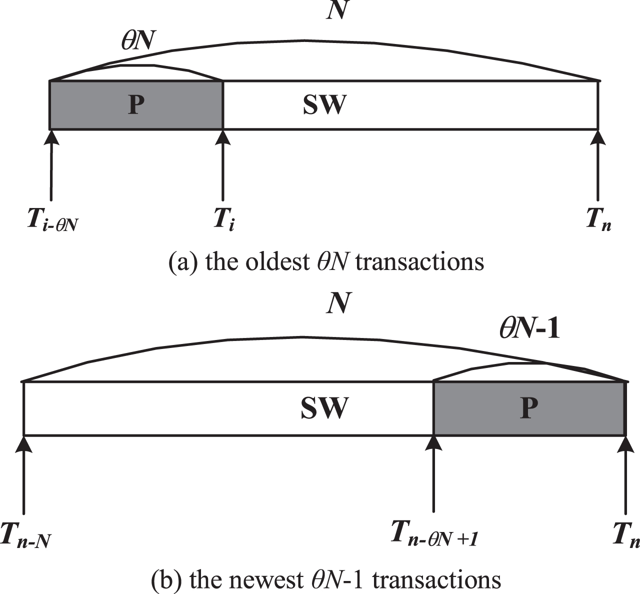
The model of mining a sliding window of data stream, (a) the oldest θN transactions, (b) the newest θN-1 transactions.

freq d ( P , T ) n = f N - θ N ( 1 + f + … + f θ N - 1 ) = f N - θ N + f N - θ N - 1 + … + f N - 1(9)

For this case, all the frequent patterns will be discovered if the minimum decay frequency can be ensured to be no smaller than (θ - ɛ) N. So, the following condition should be satisfied:□

f N - θ N + f N - θ N - 1 + … + f N - 1 ≥ ( θ - ɛ ) N(10)

According to the inequality of arithmetic and geometric means [5] as shown in Inequality 11, the Inequality 12 can be concluded. For inequality 10 and Inequality 12, we can get Inequality 13.

The upper bound of decay factor can be obtained by assumed 100% precision. Therefore the maximal decay frequency of non-frequent pattern P needs to be taken into account. That means the newest θN - 1 transactions contain P as shown in Fig. 2(b). If P is excluded from the mining result no matter how large the decay frequency of P is, then none of the other non-frequent patterns will be selected. Theorem 2 shows the upper bound for the decay factor in case of assuming 100% precision.

A k = x 1 + x 2 + … + x k k , G k = x 1 × x 2 × … × x k k ⇒ A k ≥ G k(11)

f N - θ N + f N - θ N - 1 + … + f N - 1 θ N ≥ f N - θ N × f N - θ N - 1 × … × f N - 1 θ N ⇒ f N - θ N + f N - θ N - 1 + … + f N - 1 ≥ θ N × f N - θ N × f N - θ N - 1 × … × f N - 1 θ N = θ N × f 2 N - θ N - 1 2(12)

θ N × f 2 N - θ N - 1 2 ≥ ( θ - ɛ ) N ⇒ f ≥ ( 2 N - θ N - 1 ) [ ( θ - ɛ ) / θ ] 2(13)

Theorem 2. [5] With the time decay model, precision will be 100% if the decay factor f satisfies the following condition: f < ( θ - ɛ ) N - 1 ( θ - ɛ ) N(14)

Proof. Suppose the newest θN - 1 transactions in the sliding window contain P, then the decayed frequency of P is the maximal value. The decayed frequency is shown as followed: freq d ( P , T n ) = 1 + f 1 + … + f θ N - 1(15)

To ensure that P will not be discovered, the Inequality 16 should be met. 1 + f 1 + … + f θ N - 1 < ( θ - ɛ ) N ⇒ 1 - f θ N - 1 1 - f < ( θ - ɛ ) N ⇒ 1 - f θ N - 1 < ( θ - ɛ ) N × ( 1 - f ) ⇒ 1 - f θ N - 1 < ( θ - ɛ ) N - f ( θ - ɛ ) N ⇒ f ( θ - ɛ ) N - f θ N - 1 < ( θ - ɛ ) N - 1(16)

For f^θN-1 > 0, then the following can be get. f ( θ - ɛ ) N < ( θ - ɛ ) N - 1 ⇒ f < ( θ - ɛ ) N - 1 ( θ - ɛ ) N(17)

These ways set the decay factor with considering the relationship between f and window size, minimum support and maximal error, so the scalability of the result is good. The common method sets f to lower bound with assuming 100% recall [5]. The shortage of this method is the low degree of decay and the low precision of algorithm because it only takes the 100% recall of algorithm into consideration.□

3.1. Average decay factor

This section focuses on the parameters: the sliding window size N, the minimum support threshold θ (θ ∈ (0, 1)) and the maximal support error ɛ (ɛ ∈ (0, θ)). How is the value of the decay factor f determined? Common ways usually set the decay factor to boundary values f₁ and f₂, as shown in Formula 18 and Formula 19. The value f₁, which is known as the lower bound of decay factor, can be achieved by assuming 100% recall of algorithm. The higher bound f₂ can be attained by assuming 100% precision of algorithm.

Because recall and precision cannot be 100% simultaneous, a balance of both two values should be considered when setting f. The first novel decay factor based on the average value of higher and lower bounds is proposed in this paper, which is called f _ average as shown in Formula 20. Because value 1 is much smaller than value ( θ - ɛ ) N ( [ ( θ - ɛ ) / θ ] 2 ( 2 N - θ N - 1 ) + 1 ) ,

it (value 1) can be negligible. Therefore, Formula 20 can be simplified to Formula 21. Value f₃ is the average of f _ recall and f _ precision, so the recall and precision of algorithm should be balanced in theory. Meanwhile, it avoids the randomness of setting the decay factor. f 1 = f _ recall = [ ( θ - ɛ ) / θ ] 2 ( 2 N - θ N - 1 )(18) f 2 = f _ precision = ( θ - ɛ ) N - 1 ( θ - ɛ ) N(19) f 3 = f _ average = ( f _ recall + f _ precision ) / 2 = [ ( θ - ɛ ) / θ ] 2 ( 2 N - θ N - 1 ) + ( θ - ɛ ) N - 1 ( θ - ɛ ) N 2 = ( θ - ɛ ) N ( [ ( θ - ɛ ) / θ ] 2 ( 2 N - θ N - 1 ) + 1 ) - 1 2 N ( θ - ɛ )(20) ⇒ f 3 = [ ( θ - ɛ ) / θ ] 2 ( 2 N - θ N - 1 ) + 1 2(21)

In order to further investigate the ways to set the decay factor, let us change Formula 1 to Formula 22. The function factor (f,  x) is the decay function as shown in Formulas 22 and 23. Where parameter x = m - i, i is the time of T _i arrived (i = 1, 2, …, n, …, m) and m is the time of current transaction T _m arrived. Let set D represent the accumulation of factor (f,  x), when T _m arrived the values in D are shown in Expression 24.

The forms of above decay functions are similar to factor (f, x) = f ^x . The trends of decay function values with f _ recall, f _ precision and f _ average changing over time are shown in Table 4. The values of f _ recall are the highest and the values of f _ precision are the lowest, while values of f _ average are between them.

freq d ( P , T m ) = freq d ( P , T m - 1 ) × f + r = ∑ i r i × f m - i = ∑ i r i × factor ( f , m - i )(22) factor ( f , x ) = f x(23)

D = { factor ( f , m - 1 ) , factor ( f , m - 2 ) , … , factor ( f , 1 ) , factor ( f , 0 ) } = { f m - 1 , f m - 2 , … , f 1 , 1 }(24)

In order to add the weights of recent transactions and reduce the weights of historical transactions further, the second novel way to set the decay factor on the basis of Gaussian function f ( x ) = 1 σ 2 π e - ( x - μ ) 2 2 σ 2

is proposed in this paper. It means setting decay function as factor ( f _ gauss , x ) = A σ 2 π e - ( x - μ ) 2 2 σ 2 .

To make decay function meet the characteristic of f ∈ (0, 1], constant value A is added. When the new transaction T _m arrived, the value of decay function should be 1, and decay function should associate with sliding window size N, so we set parameters the mean μ = 0 and the variance δ² = B × N, B = 1, 2, 3… Then, decay function is as follows: factor ( f _ gauss , x ) = A 2 π BN e - ( x ) 2 2 BN ,

where A > 0, B = 1, 2, 3…, N > 0. This decay function satisfies the Definition 2. Therefore, the usage of this decay function is reasonable. In conclusion, the Gaussian decay factor is shown as f₄ in Formula 25. f 4 = f _ gauss = = A 2 π BN e - 1 2 BN(25)

Example 2. Let parameters θ = 0.05, ɛ = 0.1 × θ, B = 1, 2, 3 and the values of different decay factors are shown in Table 3. For instance, f _ recall = 0.999892, f _ precision = 0.977778, f _ gauss|_B=1 = 0.9995, f _ gauss|_B=2 = 0.99975 and f _ gauss|_B=3 = 0.999833 can be achieved when N = 1K. From this table, it can be concluded that the values of f _ gauss are between values of f _ recall and f _ precision, and they are closer to f _ recall. The value of f _ gauss is bigger with B = 3 than with B = 1 under the same N. But when B = 5 and N = 1K, the value of f _ gauss is 0.9999 which is bigger than f _ recall. Therefore, set B with a large number resulting in lower degree of fade than f _ recall. It is unreasonable because we need a higher degree of fade than f _ recall. In this paper, we only consider the values of setting B to 1, 2 and 3.

The trends of decay function values with different decay factors changing over time are shown in Table 4. The values of f _ gauss are higher than f _ precision and lower than f _ recall in recent time. But in historical time the values of f _ gauss may be lower than both of them. It means that the degree of fade with f _ gauss in recent transactions is lower than the degree of fade with f _ precision. But the degree of fade with f _ gauss is higher than the degree of fade with f _ precision in historical transactions. Therefore, to set the decay factor to f _ gauss can improve the weights of new transactions and reduce the weights of old transactions.

The commonly used decay factors include: f _ d [3, 13], f_halflife [11], f_recall and f_precision [5]. This section shows the comparison between two novel decay factors we proposed and these four decayfactors.

At first, let us integrate the decay factor factor (f,  x) and get a new formula as shown in Formula 26. Parameter x = m - i is the time distance between i and m, i is the time of T _i arrived (i = 1, 2, …, n, …, m) and m is the time when current transaction T _m arrives. There are six kinds of decay functions as shown in Formula 26. When f = f _ d, f _ halflife, f _ recall, f _ precision and f _ average, its form is like the power(f, x). And f = f _ gauss, its form is like the Gaussian function.

Example 3. Let N = 10K, minimum support θ = 0.05, maximal support error ɛ = 0.1 × θ, B = 1, 2, 3, b = 2, h = 10000 [2] and f _ halflife0.93 [11]. When T₁ arrived, we can get function (f _ d, 1) =0.999930688, function (f _ halflife, 1) =0.93, function (f _ recall, 1) =0.999989, function (f _ precision, 1) =0.997778, function (f _ average, 1) =0.998884 and function (f_gauss|_B=1, 1) =0.9995. After T₄ arrived, the values of accumulation decay function in set D are as shown in Table 4. The degrees of fade are low with these decay factors expect f _ halflife after T₄ arrived. When T₅0 arrived, function (f _ recall, 50) =0.99945 which is tiny different from function (f _ recall, 1). Meanwhile, weight is 0.286505 with f = f _ gauss|_B=1 which is far lower than other values except f _ halflife. That means the weights of historical transactions are lower than other decay factors.

The values of these six kinds of decay factors with time changing are shown in Table 4 where parameters are: N = 10K, θ = 0.05, ɛ = 0.1 × θ, b = 2, h = 10000, B = 1,  2, and3. From this table it can be concluded that (1) when setting f = f _ recall and f = f _ d, there are tiny degree of fade of historical transactions with time changing as shown in Table 4. (2) When setting f = f _ halflife, there is a great degree of fade of historical transactions. (3) When setting f = f _ average, the degree of fade is between f = f _ recall and f = f _ precision. (4) When setting f = f _ gauss, the degree of fade of recent transactions is lower than f _ precision and f _ average. But the degree of fade of historical transactions is higher than these two. In other words, the feature of f _ gauss emphasizes the importance of recent transactions and reduces the importance of the historicaltransactions.

factor ( f , x ) = { = ( b - ( 1 h ) ) x = b - ( x h ) , f = f d = ( e - ( ln 2 t 1 / 2 ) ) x = e - ( xln 2 t 1 / 2 ) , f = f _ halflife = ( [ ( θ - ɛ ) / θ ] 2 ( 2 N - θ N - 1 ) ) x = ( θ - ɛ θ ) 2 x 2 N - θ N - 1 , f = f _ recall = ( ( θ - ɛ ) N - 1 ( θ - ɛ ) N ) x , f = f _ precision = ( [ ( θ - ɛ ) / θ ] 2 ( 2 N - θ N - 1 ) + 1 2 ) x , f = f _ average = A 2 π BN e - ( x ) 2 2 BN , f = f _ gauss(26)

Two novel TDMs based on f_average and f_gauss are described as Expressions 27 and 28. The value of f _ average is affected by parameters sliding window size N, minimum support threshold θ, and maximal error rate ɛ. The value of f_gauss is affected by parameters sliding window size N and B. Compared with some existing decay factors, the value of f_average is between f_recall and f_precision in order to balance the high precision and the high recall of algorithm. The character of f_gauss is that it leads to the lower degree of fade on recent transactions and higher degree of fade on historical transactions than some existing decayfactors.

freq d ( P , T m ) = ∑ i r i × ( [ ( θ - ɛ ) / θ ] 2 ( 2 N - θ N - 1 ) + 1 2 ) m - i , f = f _ average r = { 1 , if P ⊆ T m 0 , else(27)

freq d ( P , T m ) = ∑ i r i × ( A 2 π BN e - ( m - i ) 2 2 BN ) , f = f _ gauss r = { 1 , if P ⊆ T m 0 , else(28)

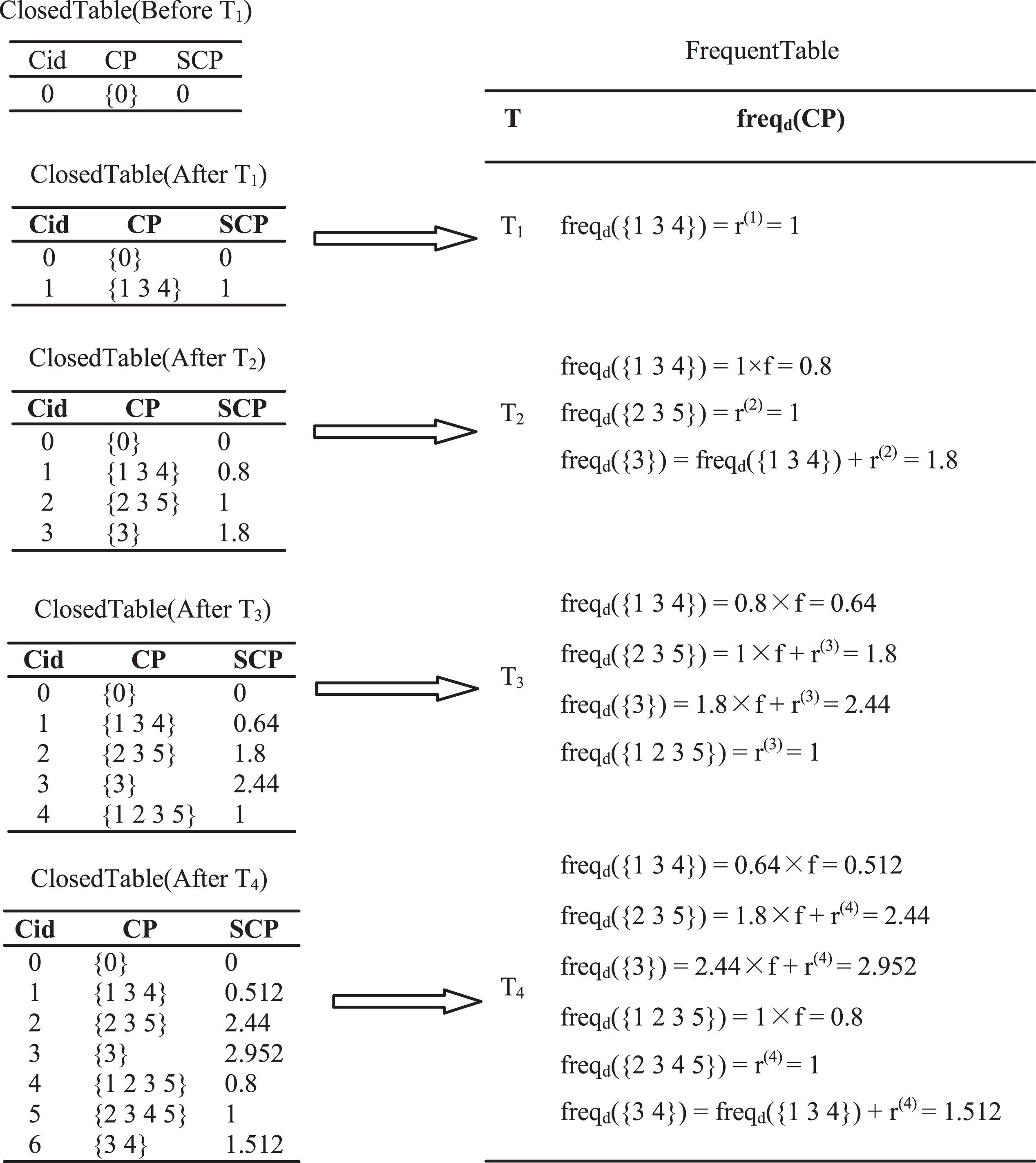
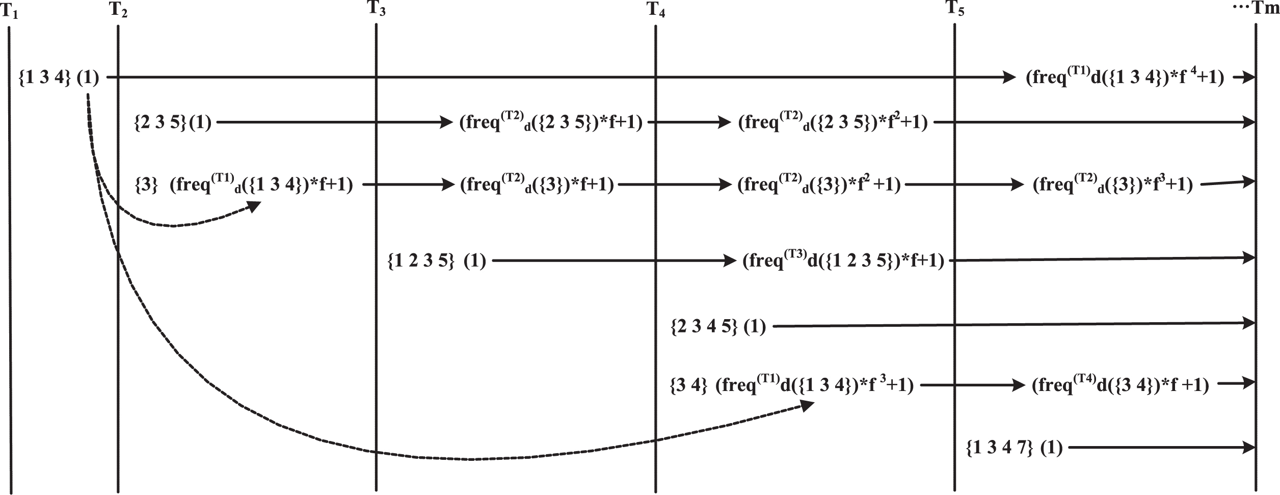
Figure 3 shows the process of generating frequent patterns based on the two novel TDMs we proposed. Each group data in Fig. 3 means < {CP} (SCP)>, where CP is the frequent itemset and SCP is the frequency of CP. There are five transactions, the first four transactions shown in Table 1 and another new transaction T₅ = {1 3 4 7}. It is different from Example 1. Instead of updating the whole ClosedTable, it updates the itemsets associated with the new transaction. For instance, the itemset <{1 3 4} (1)> is generated after transaction T₁ arrived and it only needs to be updated after transaction T₅ arrived. The frequency of {1 3 4} is updated to (1 × f⁴ + 1) which uses the value f⁴ as weight. Compared with Example 1, this proposed algorithm can reduce the time complexity when mining frequent patterns on data stream.

OPEN IN VIEWER

Fig.3

Frequent patterns mining by proposed algorithm TDMPDS.

The method we propose is called TDMPDS(TDM-based frequent Pattern mining over Data Streams). It includes adding new transactions into sliding window and dropping old transactions from sliding window. Algorithm TDMPDSADD(T _m ) is used to process the new transaction T _m , including in two main steps.

Step 1. Generate the frequent itemsets O referring to T _m and ClosedTable.

Step 2. For each frequent itemset o ∈ O.

if o is a new frequent itemset then add it to ClosedTable.

else update the frequency of o.

Algorithm TDMPDSREMOVE() is used to drop historical transactions. In order to improve the work efficiency and reduce the work time, it processes old transactions in each P steps. That means if time m % P = 0, then call the function TDMPDSREMOVE(). Its main work is to drop the non-frequent itemsets from ClosedTable.

Several methods to set the decay factors of the four algorithms are compared with each other in this paper. (1) Set f to f _ d with parameters b = 2 and h = 10000 as used in algorithm estDec [2], denoted as estDec|f _ d. (2) Set f to f_halflife with parameter t = 1 as used in algorithm UHS [11], denoted as UHS|f _ h. (3) Set f to lower bound as used in algorithm SWP [5], denoted as SWP|f _ r. (4) In order to balance recall and precision of algorithm, set f as f_average in the proposed algorithm TDMPDS, denoted as TDMPDS|f _ a. (5) To emphasize the importance of the recent transactions and reduce the weights of historical transactions, set f as Gaussian decay factor with mean μ = 0 and variance δ² = B × N, denoted as TDMPDS|f_g.

Set minimum support θ = 0.06 and 0.001 for mining out the majority of frequent patterns. The former is used to discover frequent patterns on high density data stream and the latter is used on low density data stream. Let maximal support error ɛ = 0.1 × θ, and sliding window size N = 1000, 2000, 3000 and 4000.

4.2. Performance

The first experiment analyzes the parameter B of Gaussian decay factor. Figure 4 shows the performance of algorithm TDMPDS on high density data stream msnbc. The comparison among parameters B = 1,  2,  3 can achieve the best precision and the worst recall if B = 1, and the best recall and the worst precision are obtained by B = 3. The analysis of performances under different sliding window sizes shows that, if B = 3 the optimal performance of algorithm and the most balanced recall and precision are achieved as shown in Fig. 4(c). The performance is followed by setting B = 2, while the maximum gap between recall and precision of algorithm is obtained with setting B = 1. Dealing with the low density data stream Kosarak, it can also get similar conclusions.

OPEN IN VIEWER

Fig.4

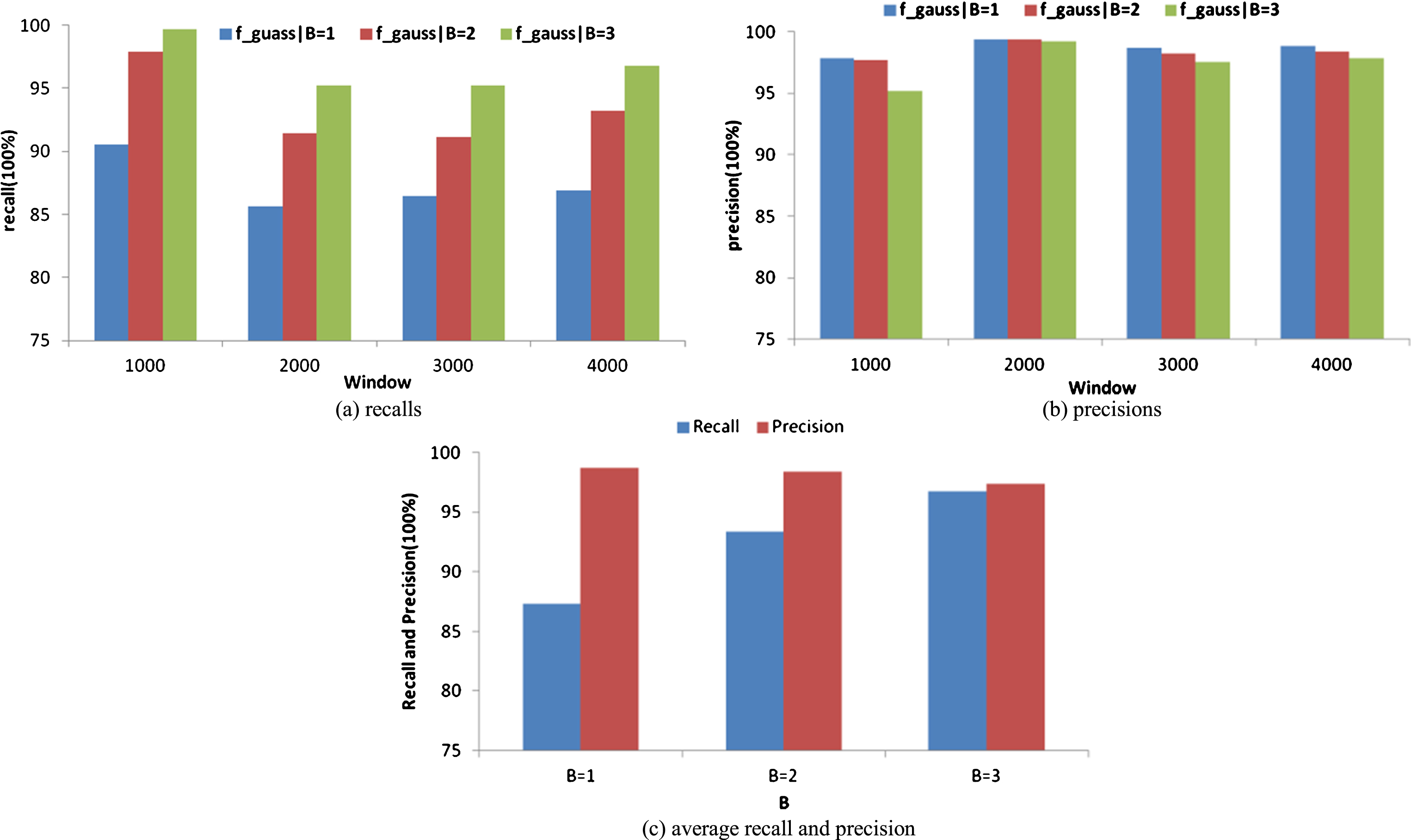
Variation of recall and precision with different Bs and windows on msnbc, (a) recalls (b) precisions (c) average recall and precision, (a) recalls with different windows (b) precisions with different windows.

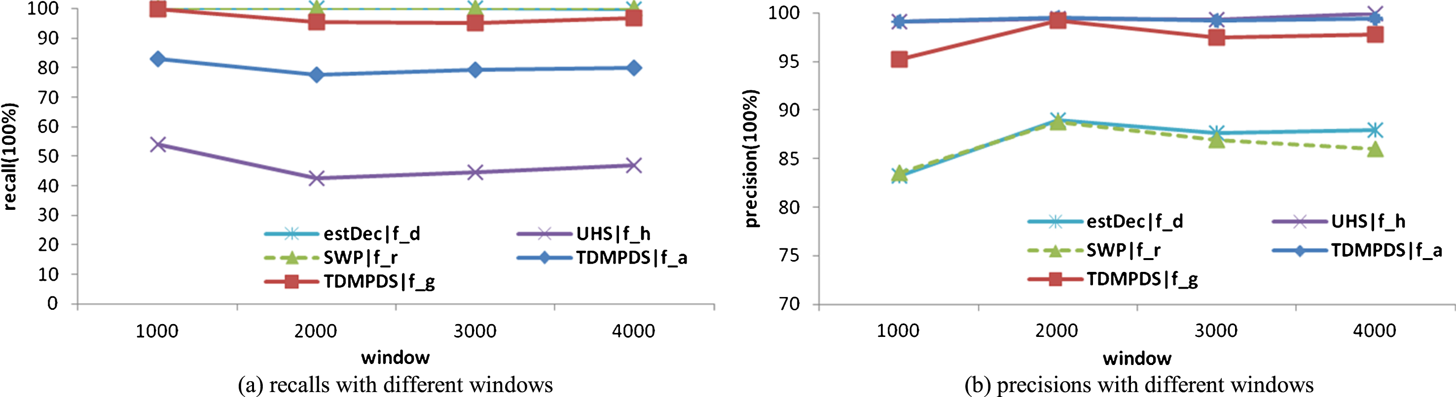
Next, compare the pros and cons of different decay factors of the four algorithms over high density data stream msnbc. Let B = 3, the performances of algorithms are shown in Fig. 5. It can be concluded that: (1) performances of algorithm are less influenced by sliding window sizes for TDMPDS|f_a andTDMPDS|f_g. (2) It gets almost 100% recalls for SWP|f_r and estDec|f_d. However, the corresponding precisions are the lowest two. (3) The highest precision is obtained by USH|f_h. But the corresponding recall is the lowest. (4) The recall for TDMPDS|f_a is lower than recall for SWP|f_r, while the precision is higher than it. (5) Average value of recall and precision for TDMPDS|f_g is optimal compared with other ways.

OPEN IN VIEWER

Fig.5

Performance comparison for different methods on msnbc, (a) Kosarak (b) Bmswebview.

To sum up, in Figs. 5 and 6, the performances of algorithms on msnbc ranging from being excellent to poor are: TDMPDS|f_g ⟶ estDec|f_d ⟶ SWP|f_r ⟶ TDMPDS|f_a ⟶ UHS|f_h. In detail, the performances for estDec|f_d and SWP|f_r are almost the same. The average of recall and precision for UHS|f_h is 21% lower than SWP|f_r, the performance for TDMPDS|f_a is about 3% lower than SWP|f_r, and the performance for TDMPDS|f_g is about 5% higher than SWP|f_r.

OPEN IN VIEWER

Fig.6

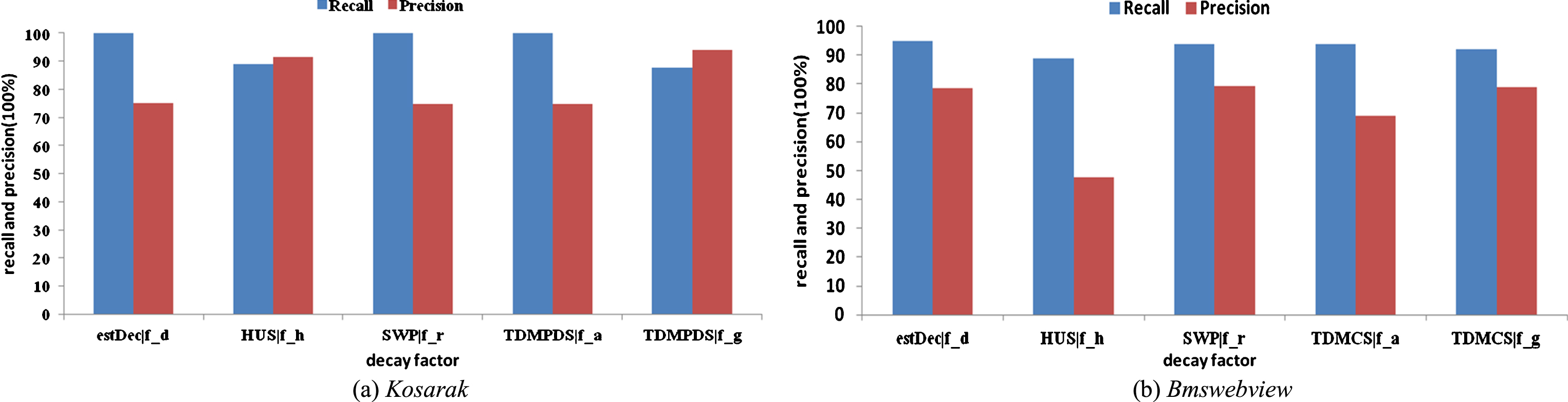
Comparison of average recall and precision for the different methods on Kosarak and B mswebview, (a) recalls with different windows (b) precisions with different windows.

The second experiment deals with low density data stream Kosarak and Bmswebview, the performances of algorithms are shown in Fig. 6. The performances of algorithms on Kosarak ranging from being excellent to poor are: TDMPDS|f_g ⟶ TDMPDS|f_a ⟶ UHS|f_h ⟶ estDec|f_d ⟶ SWP|f_r. In detail, the performances for estDec|f_d and SWP|f_recall are almost the same. The performances of algorithms on Bmswebview ranging from being excellent to poor are: SWP|f_r ⟶ TDMPDS|f_g ⟶ estDec|f_d ⟶ TDMPDS|f_a ⟶ UHS|f_h. In detail, the performances for TDMPDS|f _ g and SWP|f_r are almost the same.

The third experiment processes synthetic data streams, the performances of algorithms are shown in Fig. 7. Four data streams with different lengths of transactions or patterns are used, including: T10I4, T10I5, T10I10 and T20I5. Therefore, the performances of algorithms ranging from being excellent to poor are: TDMPDS|f_g ⟶ estDec|f_d ⟶ SWP|f_r. In detail, the performances of estDec|f_d and TDMPDS|f_a are almost the same, and the average values of recall and precision of UHS|f_h are lower than other algorithms.

OPEN IN VIEWER

Fig.7

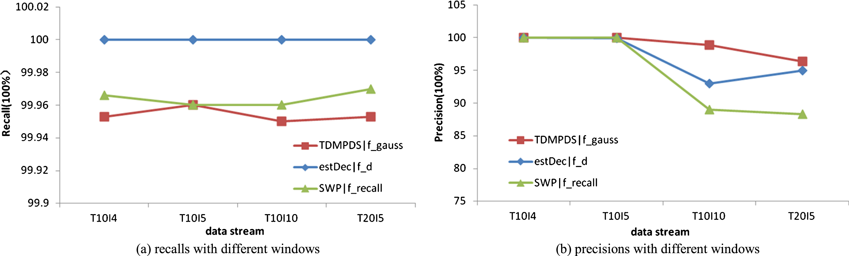
Performance comparison for the different methods on synthetic data streams.

From all the experiments above mentioned, we can draw the following conclusions:

The changing of sliding window size has less influence on the performances of algorithms with f_a and f_g.