Feature selection from high dimensional data based on iterative qualitative mutual information

Abstract

High Dimensional cancer microarray is devilishly challenging while finding the best features for classification. In this paper a new algorithm is proposed based on iterative qualitative mutual information to choose the features that can provide optimal feature set with reliability, stability, and best classification results. It finds the qualitative (i.e. utility) score of each feature with the help of Random Forest algorithm and combines it with mutual information of each feature with its class variable. Adding a qualitative measure along with mutual information can improve the robustness and find redundant features in data. The proposed algorithm has been compared with other representative methods through the ten microarray based cancer datasets in terms of number of features and classification accuracy of three well-known classifiers: Naïve Bayes, IB1 and C4.5. Experimental results show that the proposed approach is effective in producing an optimal feature subset and improves the accuracy of these datasets.

Keywords

Feature selection microarray classification wrapper filter model random forest mutual information

1. Introduction

Today, the data available are high Dimensional in nature and this nature of data has become a significant issue. The size of the available datasets is high in terms of both the number of features in each sample and the number of data samples [45]. There has been a lot of research going on high dimensional microarray data. Microarray datasets have a characteristic of having large number of genes but very less number of samples, which leads to an unsound application of classification methods [12, 37].

Many of researchers [7 , 43] have shown that the high dimensional data sets contain redundant and irrelevant genes and these redundant genes greatly affect the performance of the classifier. So, in order to improve the performance of the classifier and remove the redundant features, feature selection has become an important task in case of microarray data.

In literature, feature selection methods are classified into four categories: Filter approach, Wrapper approach, Embedded and Hybrid approach [15 , 28]. In Filter feature selection, feature subset is preprocessing step before applying any learning and classification process. In the Wrapper method [25], like genetic algorithm, features are selected in accordance with the learning algorithm. It gives better feature subset than filter approach as it is tuned according to the algorithm. However, it is much slower than filter feature selection.

When the number of features becomes very large, the filter model is preferred due to its computational efficiency and simplicity [28]. Another feature selection method is the embedded approach. These methods solve the problem of overfitting which is persistent in case of wrapper methods. Examples for embedded methods are Artificial Neural Network (ANN) and Random Forest (RF).

Using the filter feature selection approach, many algorithms were proposed such as Relief [24], Relief-F [26], FOCUS, FOCUS-2 [1], Correlation based Feature Selection (CFS) [16], Fast Correlation based feature selection (FCBS) [28], Fast Clustering-Based Feature Subset Selection Algorithm (FAST) [32]. Hoque et al. [17] has proposed a greedy filter feature selection method based on mutual information of variables. There method MIFS-ND selects high ranked features using an optimization criterion of NSGA-II algorithm. Although this approach provides good predictive performance for most of the datasets, is not performing well with cancer datasets such as Colon. Jain and Murthy [22] have proposed a new estimation measure called Mutual Information Based Dependence Index (MIDI), which is an estimate over existing mutual information based dependence measure. This measure has overcome the limitations found in measures like Distance Correlation (dcor), Maximal Information Coefficient (MINE). Some of the filter methods such as FCBS [28], FAST [43] utilize the information theoretical concept to solve the problem of feature selection. They find feature to class relevance and feature-feature correlation with the help of mutual information and symmetric uncertainty. They give a good subset of features, but it is difficult to decide a threshold value for a relevant feature. One of the drawbacks of FCBF is that it considers pair wise correlation between the features. FAST Algorithm creates clusters, which uses Minimum Spanning tree to remove the problem of redundancy. This leads to an increased computational cost in high dimensional data.

Mortazavi and Mottar [33] tried to improve the stability and robustness in the scarce microarray data and proposed a method using a cooperative game theory framework based on Shapley value. The author of [29] has defined a Qualitative-quantitative measure of mutual information for Multi-modal image registration. The measure is formed by adding a utility function into the conventional mutual information. They have related the probability occurrence of event with its utility. Even though they have proved its improvement over the conventional mutual information but it becomes computationally expensive when number of features is very large. Calculating QMI of each feature with every other feature in the high dimensional dataset becomes infeasible.

Biau and Scornet [5] have shown that ranking the features using random forest performs excellent when the number of features is much larger than the sample. Uriarte et al. [11] have proved that random forest can be easily used for classification of microarray data. Random Forests are applied as they identify important variables and can achieve high classification accuracy. This property has made them very popular for high dimensional data analysis. Random forests (RF) [8] is a popular tree-based ensemble machine learning tool that is highly data adaptive, applies to “large p and small n” problems, and can account for correlation as well as interactions among features [9].

Filter feature selection methods such as chi-square, ANOVA do not remove multi-collinearity. Random Forest helps to solve the problem of multi-collinearity. It is useful in finding correlation among features. The importance score of random forest separates the correlated features by giving higher importance to one of them and other correlated features have very low importance score. Therefore, RF importance score can be helpful in separating the correlated variables. Using this property, this paper finds the share of preference for each variable (Preference Score).

The random Forest algorithm has still some shortcomings; it does not perform well for classification on imbalance data. The data obtained in reality are in the form of the samples obtained from different categories (or class), this makes the data imbalance. Most classifiers perform poorly as they are biased to large samples. Similar to standard classifiers, Random forest does not work well when the data imbalance is extreme. However, this problem can be mitigated if some solutions are applied to random Forest [4]. RF performs poorly for classification on imbalance data. The imbalanced data causes the training set for each decision tree to be imbalanced during the first “random” procedure [30].

Motivated by this, the paper defines a new algorithm that initially balances the dataset. Then it defines a feature selection method, which uses a qualitative measure of mutual information for robust and stable feature subset. Qualitative mutual information (QMI) is used, as it not only considers the effect of mutual information of each variable with class, but also considers the Qualitative aspects (utility) of each feature. This paper is an extended version of the work published in [35]. The algorithm discussed here is explained step by step with an initialization phase added to it. The experimental results in this paper are discussed more clearly with more number of datasets. The comparison of results is also performed with other existing relevant and latest algorithms.

The rest of the paper is organized as follows: Section 2 the proposed algorithm is presented through Algorithm 1. Section 3 outlines experimental results, of proposed algorithm with other existing algorithms on different cancer microarray datasets. Analysis of result using different parameter setting is discussed in section 4. The statistical test used for comparison is covered in Section 5. Section 6 concludes the paper.

2. Proposed method

To obtain a stable subset of genes from high dimensional microarray datasets even in the presence of class imbalance and scare data a new gene selection algorithm is proposed which uses a qualitative measure of mutual information (QMI). The proposed algorithm consists of three phases. These phases are initialization phase, intermediate feature selection phase and final phase. The working of these phases is depicted in Algorithm 1. The initialization phase is added in comparison to the QMI method discussed in [35] so as to reduce the computations of the next phase. The intermediate feature selection phase combines the balancing stage and intermediate feature selection stage explained in paper [35] into one phase. The output in the form of reduced number of genes is obtained from the final phase.

2.1. Algorithmic description

The underlying paradigm of the proposed gene selection algorithm is to provide a stable genes subset when the available data has limited sample size and classes are imbalance. Unlike existing gene selection method, it selects a candidate gene which has high relevance with target class and low redundancy among the selected genes. The complete proposed algorithm is presented through Algorithm 1. It is a three phases algorithm with one single dataset including class label as its input. The first phase is the Initialization phase where the Non-dominated solutions (NDS) is initialized to be empty set (null). NDS is the solution set, in which every solution is different in terms of number of features and accuracy. Suppose there are two solutions S1 and S2, S2 is non-dominated by S1 if |S1| ≤ |S2| and accuracy (S1) >accuracy (S2). ‘numIter’ is the input parameter which can control the number of solutions found in NDS. The important role of this phase is to calculate the Mutual information (MI) [10] for each gene individually with the class/ target variable in the dataset. Mutual information of each feature with class can help to remove irrelevant features.

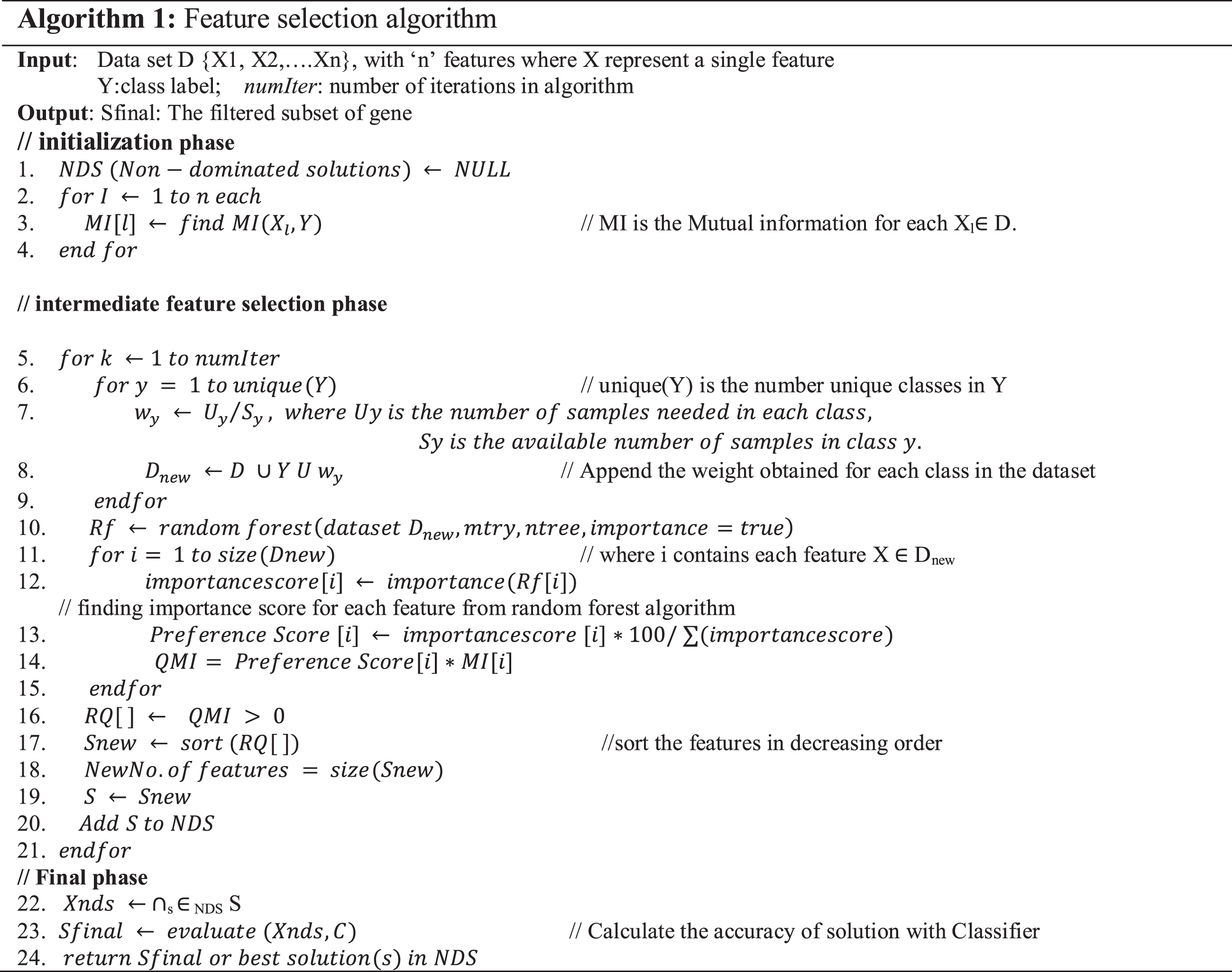
The next phase is the intermediate feature selection phase of the algorithm. This collects each candidate gene subsets with low redundancy and high relevance in a set of Non-dominated solutions (NDS). At each iteration (k), construction step adds a new solution to the NDS. The single iteration of the Construction step is a sixteen-step procedure, in which the first four steps balances the obtained Dataset D and in other steps feature reduction is performed.

In the first four steps, the proposed algorithm solves the problem of class imbalance and balances the obtained data by incorporate class weights for each class in the dataset. The weights are calculated for each class so that the number of samples representing the one class can come in line with the number of samples representing other class. The weighting factor which balances both classes can calculate as the ratio of proportions needed in each class with the actual proportion of sample in each class in the data. Weighting is done as per the following equation: $W_{i} = \frac{U_{i}}{S_{i}}$ (1)

W_i is the weight obtained for class i. U_i is the number of required sample in each class of the dataset. S_i is number of actual samples available in dataset representing the class i.

To balance the dataset, generally the value of U_i remains the same for all classes. This technique becomes useful when we want the small sample in each class could represent the population of that class. After successfully completion of the weighting methodology the data set is transformed from imbalance state to balance state without changing the actual values of the dataset. The data of the obtained samples is not changed and is balanced before considering it as an input to the algorithm.

The balanced dataset is given as input to the Random forest algorithm. Random forest algorithm is used to find the importance score of each feature. Importance score of random forest gives importance to features in such a way that collinearity between them is reduced. In other words, if one feature is given highest importance than the importance of other correlated features is greatly reduced. To get the actual rank of each feature in comparison to all other features, the algorithm computes the preference score of each feature. The preference score of each feature gives the weight to each feature corresponding to other features in the dataset. Preference Score of a feature Xi is weightage obtained by Xi relative to all other features. It is given in Equation (2) $\begin{matrix} Preference Score [Xi] = importancescore [Xi] \\ \times 100 / \sum (importancescore) \end{matrix}$ (2)

Where, importancescore is the value of the importance score obtained from random forest algorithm.

Further, these preference scores are utilized as utility function in calculating the QMI value for each gene. Qualitative measure of mutual information (QMI) is formed by adding a utility function into the conventional mutual information. The utility value for each feature has been found by preference score. Preference score has the property that it helps to distinguish correlated features. The Mutual information helps in providing the gain of each feature with class variable. Irrelevant features will always have lesser gain with class variable. Therefore, combing both can reduce irrelevant as well as redundant features from the dataset.

Let ‘n’ be the total number of features in the Dataset D{ X1, X2, … Xn } with X defining a feature. Preference score of each feature be PS1, PS2, … .PSn, QMI of each feature ‘Xi’ is defined as $QMI (X_{i}) = {PS}_{i} \sum_{i = 1}^{n} P (X_{i}, C) log \frac{p (X_{i}, c)}{X_{i}}$ (3)

Where, $\sum_{i = 1}^{n} P (X_{i}, C) log \frac{p (X, C)}{X_{i}}$ is the mutual information of feature X_i with the class variable ‘C’.

This means that the feature will be appropriate if its QMI value increases. QMI gives only those features whose relevance with the class is greater and its redundancy with other features is reduced. This value helps in obtaining the discriminating value for each feature.

The new rank of genes is based on QMI value and genes whose rank is greater than zero are the subset of genes obtained after removing irrelevant and redundant features. Array ‘RQ’ in algorithm1 keeps all the genes whose rank is greater than zero. ‘RQ’ is further sorted in Descending order to keep the highest-ranking genes at the top. This is the feature reduction step where the genes/features with rank zero or less than zero are removed and others with score greater than zero are kept as relevant ones in array Snew. This subset of feature in Snew at 1st iteration (k = 1) is one of the reduced subset and it is added to NDS. For other iterations, same procedure is followed and all the solutions found are added to NDS.

The final phase of the algorithm 1 helps to obtain the final gene subset from all the subsets in NDS which can provide best accuracy for the dataset. In the final Phase of the algorithm, the result obtained in the construction phase are analyzed. ‘S’ is the individual solutions obtained in NDS. This step finds the common genes found in all solutions to obtain the best and stable gene set. Then the accuracy of the new obtained subset is found using a classifier ‘C’. The obtained solution set is the final subset of candidate genes.

3. Implementation and results

3.1. Experimental setup and dataset description

The effectiveness of the proposed algorithm is demonstrated here for the ten standard cancer microarray datasets of high dimensionality. Breast, Colon, leukemia, prostate and lung cancer datasets are obtained from Kent Ridge Biomedical Data repository [40] and are described in Table 1.

Table 1
Dataset description

Dataset Samples Original genes Preprocessed genes Classes

Colon_1 37 22883 8826 2

Prostate 102 12600 5966 2

Breast 97 24482 5000 2

Colon 62 2000 2000 2

SRBCT 83 2308 2308 4

Endometrium 42 8872 3000 4

Leukemia 72 7129 7129 3

Melanoma 38 8076 8076 3

CNS-v1 34 7129 2277 2

Lung 32 12533 12533 2

Dataset	Samples	Original genes	Preprocessed genes	Classes
Colon_1	37	22883	8826	2
Prostate	102	12600	5966	2
Breast	97	24482	5000	2
Colon	62	2000	2000	2
SRBCT	83	2308	2308	4
Endometrium	42	8872	3000	4
Leukemia	72	7129	7129	3
Melanoma	38	8076	8076	3
CNS-v1	34	7129	2277	2
Lung	32	12533	12533	2

Breast Cancer Data: The obtained data has 97 samples and 24482 genes. Number of samples belong to two classes with 51 samples are those patients who remained healthy from the disease at least for 5 years after initial diagnosis and 46 are those who developed distance metastases within 5 years. A preprocessing procedure has been applied on the data. Attributes with more than 30% of the missing values are removed. Other attributes containing null values are replaced with the class wise mean. Finally, 5000 genes with highest variance are selected.

SRBCT Cancer Data: This data has been obtained from Khan Dataset [20]. It has 83 samples divided into four classes, 29 EWS samples, 18 NB samples, 11 BL samples, and 25 RMS samples.

Endometrium Cancer Data: This data consists of 42 samples and 8872 genes [41]. The genes with more than 30% of the missing values are removed and remaining missing values are replaced by their class wise mean. Finally, 3000 genes are left for experiments. It has four classes of samples which are 13 serous papillary, 3 clear cell, 19 endometrioid cancers,7 age-matched normal endometria samples.

Melanoma Cancer Data: It is collected and given in [6]. It consists of 38 samples and 8076 genes. It is three class dataset where the three classes of sample are 12 Lentingo samples, 19Acral samples, 7 Nodular samples.

CNS-v1 Cancer Data: This data consists of 34 samples and 7129 genes [38]. A preprocessing technique is used which is like that given by Yang et al. [23] is implemented. To filter the genes Max/Min ratio of 5 and Max-Min difference of 500 is set across the samples. The cut-off value was set between 20–16000. The value below and above this range are discarded. Finally, number of genes left are 2277. Its samples belong to two classes, 9 Normal samples class, 25 brain tumor samples class.

Colon-I Cancer Data: Samples collected for this dataset is 37 with two classes, 8 Normal patient samples and 29 tumor samples It has 22883 original genes [27]. A preprocessing technique given by Yang et al. [23] is implemented and the cut off value ranges between 20–16000. The genes with Max-Min difference of 100 across the samples are not discarded. After filtering number of genes left are 8826.

Prostate Cancer Data: This data has 102 samples belonging to two classes, 52 prostate tumor samples and 50 Normal samples. Original number of genes are 12600 and preprocessing number of genes left are 5966. For filtering out the genes with missing value, the minimum cut off value of 100 and a maximum cutoff value of 16000 with a variation of the Max/Min ratio as 5 and Max-Min difference of 50 was utilized.

In all these datasets, all genes are numerical values and are normalized using z-score normalization before using them in the experiments.

The proposed algorithm has been implemented and compared with some of the other feature selection algorithms such as Fast Correlation based feature selection (FCBS) [28], Fast Clustering-Based Feature Subset Selection Algorithm (FAST) [43], Random Forest Statistical Test (RFST) [34] and Random Forest (RF) [14].

While experimenting with random forest algorithm two parameters are needed to be defined, they are mtry i.e., the number of input variables randomly chosen to generate tree and ntree i.e., the number of trees in the forest. The values of these parameters are kept as their default values, ntree = 5000, $mtry = \sqrt{n}$ , where n is the number of features. Uriarte [11] has suggested that default values are a good option with just a little variation in time of execution. In the implementation of the algorithms such as RF, RFST and proposed QMI algorithm the same parameter values have been designated for comparison purposes.

3.2. Results and comparison

The performance of the proposed algorithm has been compared with other existing feature selection algorithms in terms of the number of relevant genes, and classification accuracy. The results are presented through Table 2. In Table 2 for each classification algorithm the average classification accuracy is found using 10-fold cross validation strategy for the training and testing set on all data sets. While comparing the algorithms, the one with higher accuracy is a better algorithm than the other. In case of same accuracies, the one which selects less number of features is preferred.

Table 2
Comparison of classification Accuracy and number of genes selected with four existing feature selection algorithms

Dataset	Classifiers	Accuracy (10 fold)
Dataset	Classifiers	Full set	FCBF	FAST	RF	RFST	Proposed
Colon_1 (Two Class)	Naïve Bayes	81.08	42.4(15)	65.64(16)	97.29(63)	100 (11)	100 (20)
	C4.5	94.59	89.18(15)	70.14(16)	97.20(63)	97.29(11)	97.29(20)
	IB1	78.37	81.08(15)	80.47(16)	97.20(63)	97.29(11)	100(20)
Prostate (Two Class)	Naïve Bayes	62.74	83.33(77)	93.77(19)	82.35(19)	72.54(32)	93.13(69)
	C4.5	75.49	89.21(77)	89.87(19)	81.37(19)	80.39(32)	85.29(88)
	IB1	86.27	78.43(77)	86.55(19)	90.19(19)	90.19(32)	94.11(69)
Breast (Two Class)	Naïve Bayes	59.79	59.79(99)	65.71(16)	69.07(42)	71.13(12)	82.47(39)
	C4.5	57.73	52.57(99)	58.68(16)	58.04(42)	60.82(12)	80.41(23)
	IB1	58.76	67.01(99)	73.19(16)	74.28(42)	75.60(12)	90.72(98)
CNS-v1 (Two Class)	Naïve Bayes	73.29	74.70(35)	75.23(20)	87.05(21)	88.23(19)	94.11(12)
	C4.5	70.58	67.01(35)	73.19(20)	82.35(21)	85.29(19)	76.47(12)
	IB1	76.47	70.58(35)	81.21(20)	87.05(21)	91.17(19)	100(14)
Colon (Two Class)	Naïve Bayes	51.61	64.51(34)	95.08(14)	75.80(26)	95.48(17)	85.48(28)
	C4.5	69.35	64.51(34)	90.40(14)	80.64(26)	79.03(17)	87.09(27)
	IB1	62.90	58.06(34)	66.12(14)	80.25(26)	80.64(17)	87.09(68)
Lung (Two Class)	Naïve Bayes	96.85	3.03(50)	77.61(22)	100(312)	100(18)	100(23)
	C4.5	71.87	36.36(50)	88.56(22)	90.62(312)	93.75(18)	96.87(23)
	IB1	96.85	57.57(50)	98.21(22)	100(312)	100(18)	100(23)
Melanoma (Three Class)	Naïve Bayes	47.36	50(43)	42.67(29)	50(7)	63.15(25)	55.26(8)
	C4.5	50	65.78(43)	70.04(29)	57.89(7)	78.95(25)	73.68(18)
	IB1	50	47.36(43)	62.63(29)	73.68(7)	86.84(25)	78.94(18)
Leukemia (Three Class)	Naïve Bayes	64.44	72.77(12)	100(15)	98.61(16)	100(10)	98.61(31)
	C4.5	94.44	52.77(12)	100(15)	94.44(16)	100(10)	94.44(31)
	IB1	83.33	56.94(12)	100(15)	94.44(16)	100(10)	97.22(31)
SRBCT (Four Class)	Naïve Bayes	86.74	83.13(10)	89.23(5)	97.59(13)	98.79(8)	98.79(8)
	C4.5	73.49	72.28(10)	77.69(5)	86.74(13)	85.54(8)	87.43(10)
	IB1	83.13	84.33(10)	73.33(5)	100(13)	100(8)	98.79(15)
Endometrium (Four Class)	Naïve Bayes	80.95	52.38(1)	72.31(12)	80.33(14)	80.95(8)	85.71(44)
	C4.5	57.14	61.90(1)	69.88(12)	66.66(14)	71.42(8)	76.19(29)
	IB1	90.47	59.52(1)	67.33(12)	75.71(14)	78.57(8)	90.47(90)

The highest accuracy values for each dataset corresponding to each classifier are marked in boldface. The number of genes in the proposed algorithm gives the sufficient number of genes which are the best in predicting the disease. On this subset, the algorithms give the best average accuracy for these datasets. The results obtained in Table 2 are summarized as follows:

Naïve Bayes and IB1 classifier achieves a maximum classification accuracy of 100% for Colon-1 dataset by the proposed QMI algorithm. Naïve Bayes classifier achieves 100% accuracy with our previously proposed algorithm RFST. Its accuracy is 42.4%, 65.64%, 97.29% for FCBF, FAST and RF respectively. C4.5 classifier obtains 97.29% classification accuracy with 20 selected features for QMI algorithm.

In Prostate dataset the features selected using QMI algorithm achieves IB1 classification accuracy of 94.11% with 69 selected features which is significantly better than other algorithms. The Naïve Bayes and C4.5 classification accuracies of 93.77% and 89.87% respectively obtained on FAST algorithm are slightly better than the Naïve Bayes and C4.5 accuracies of 93.13% and 85.29% respectively on QMI dataset. This because this dataset creates the problem of data over fitting.

The classification accuracy of Naïve Bayes, C4.5 and IB1 classifier is 82.47 %, 80.41% and 90.72% respectively for Breast dataset on selected features obtained by the proposed QMI algorithm.

CNS-v1 dataset for QMI algorithm in Naïve Bayes and IB1 classifier achieves 94.11% and 100% accuracy. This has brought a significant improvement than existing algorithms.

The Naïve Bayes, C4.5 and IB1 classifiers have reported 85.48%, 87.09% and 87.09% accuracies for proposed QMI algorithm on Colon dataset. The accuracy of classifier for RFST feature selection algorithms is 95.48%, 79.03% and 80.64%.

The Naïve Bayes and IB1 achieve a classification accuracy of 100% for Lung dataset on the features selected by the proposed algorithm QMI and RFST algorithms. Their C4.5 classifiers accuracy is 96.87% and 93.75% as presented in Table 2.

Among the three class datasets Melanoma and Leukemia, the classification accuracy reported by RFST algorithm is better than other algorithms. Since QMI algorithm is not able to handle the samples which are from three different classes, it is not performing well for these data sets. In case of Leukemia dataset, feature subset obtained by RFST algorithm reports 100% classification accuracy.

In case of SRBCT dataset classification accuracy of Naïve Bayes classifier is 98.79% for features selected using QMI algorithm. This is highest accuracy among all the other feature selection algorithms. The classification accuracy for FCBF, FAST, RF and RFST is 83.13%, 89.23%, 97.59% and 98.79% respectively as shown in Table 2. The C4.5 and IB1 classifier achieves 87.43% and 98.79% accuracy with QMI algorithm.

The proposed algorithm QMI shows an impressive improvement for Endometrium dataset with Naïve Bayes, C4.5 and IB1 classification accuracy of 85.71%, 76.19% and 90.47% respectively as against the RFST algorithms classification accuracies of 80.95%, 71.42% and 78.57%

Some of the recently proposed gene selection algorithms available are also used for comparing the proposed algorithm. Table 3 lists such a comparison in terms of number of genes and classification accuracy along with the source of the algorithm. It represents the average accuracy of each algorithm with the number of genes being represented within the parenthesis.

Table 3

Comparison of proposed algorithm with other state of art algorithms

Dataset	Alogithms	Accuracy & No. of features
Colon	Proposed+IB1	87.09(68)
	BBF+SVM [46]	90.32 (12)
	MI+SVM [44]	74.19(23)
	mRMR-ABC+SVM [3]	94.17(20)
Breast	Proposed+IB1	90.72(98)
	POS+KNN [31]	66.8(11)
	POS+SVM [31]	68.7(22)
SRBCT	Proposed+NB	98.79 (8)
	Proposed+NB [33]	97.27
	POS+KNN [31]	99.5(22)
	POS+SVM [31]	99.7(8)
	mRMR-ABC+SVM [3]	96.30(10)
Colon_1	Proposed+NB	100(20)
	Irgon et al. [19]	95.5
Lung	Proposed+NB	100(23)
	mRMR-ABC+SVM [3]	98.95(8)
	Proposed+NB [33]	92.35
	Proposed+Decision tree [33]	85.42
CNS-V1	Proposed+IB1	100(14)
	SVM-RFE+SVM [2]	75.49(100)
Prostate	Proposed+IB1	94.11(69)
	MDS+SVM [39]	94.32
	Proposed+NB [33]	90.12
	Irgon et al (2010)	99.8
Leukemia	Proposed+NB	98.61(93)
	MGS-CM+SVM [42]	90.97
	MDS+SVM [39]	96.75
	Alonso et al. [2]	78.22(100)
	POS+KNN [31]	99.5(1)
	POS+SVM [31]	99.5(1)
Endometrium	Proposed+IB1	90.47(90)
	HGPA [32]	42
	CSPA [32]	55

It can be verified from Table 3 that the proposed algorithms accuracy on IB1 classifier is highest when compared with BBF algorithm on SVM classifier [46] and MI algorithm on SVM Classifier [44]. It can be observed that the proposed algorithm tends to provide better accuracy results than one of the algorithms proposed by Mortazavi & Moattar [33].

4. Analysis of experimental result

The proposed algorithm defined in Algorithm 1 uses a control parameter ‘numIter’ that is the Number of iterations of the construction phase. In order to check at which iteration, the selected genes can give us the best accuracy with minimum number of genes, the algorithm is run at numIter value ranging from 2 to 50. This is important to identify the stable gene subset, which could deliver higher performance. Figs. 1–9 depicts the classification performance corresponding to number of genes selected at numIter values from 2 to 30 for three of the classifiers (Naïve Bayes, IB1 and C4.5). A 10-fold cross validation accuracy is employed to disclose the results of the changing parameter. In each figure, every point indicates the number of genes and corresponding accuracy at each ‘numIter’ value of the algorithm. The three different lines indicate the three different classifiers.

Fig. 1

Gene selected corresponding to accuracy for Colon_1.

Fig. 2

Gene selected corresponding to accuracy for Endometrium.

Fig. 3

Gene selected corresponding to accuracy for Prostate.

Fig. 4

Gene selected corresponding to accuracy for CNS V1.

Fig. 5

Gene selected corresponding to accuracy for Leukemia.

Fig. 6

Gene selected corresponding to accuracy for Breast data.

Fig. 7

Gene selected corresponding to accuracy for SRBCT.

Fig. 8

Gene selected corresponding to accuracy for Melanoma data.

Fig. 9

Gene selected corresponding to accuracy at different iterations for Colon data.

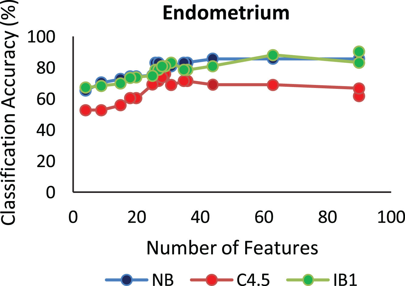
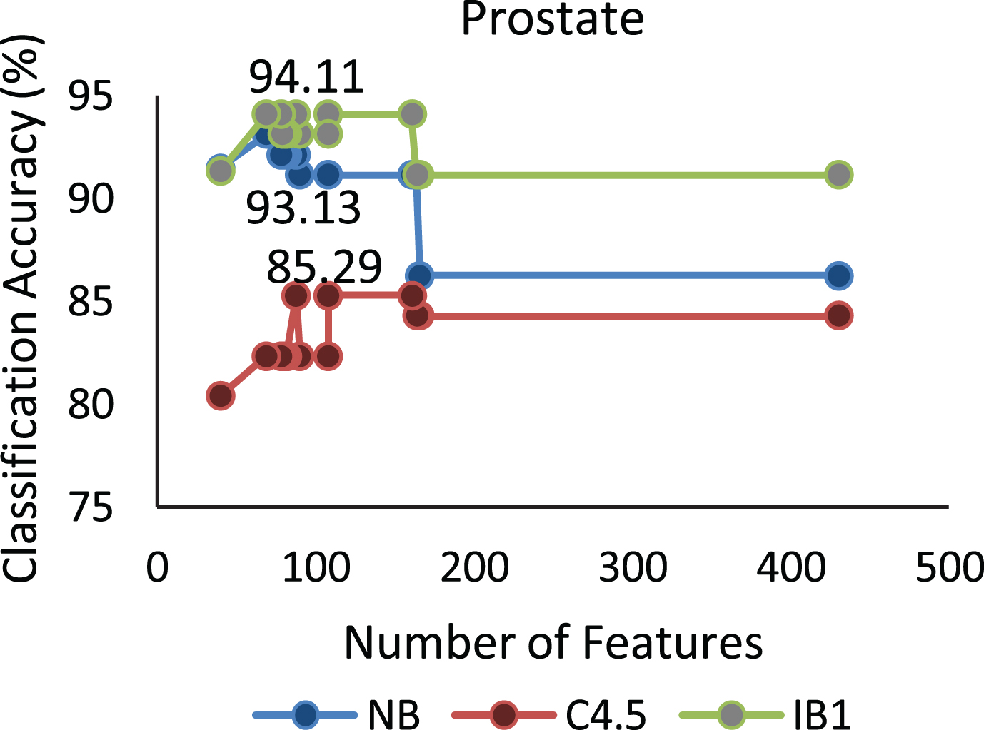
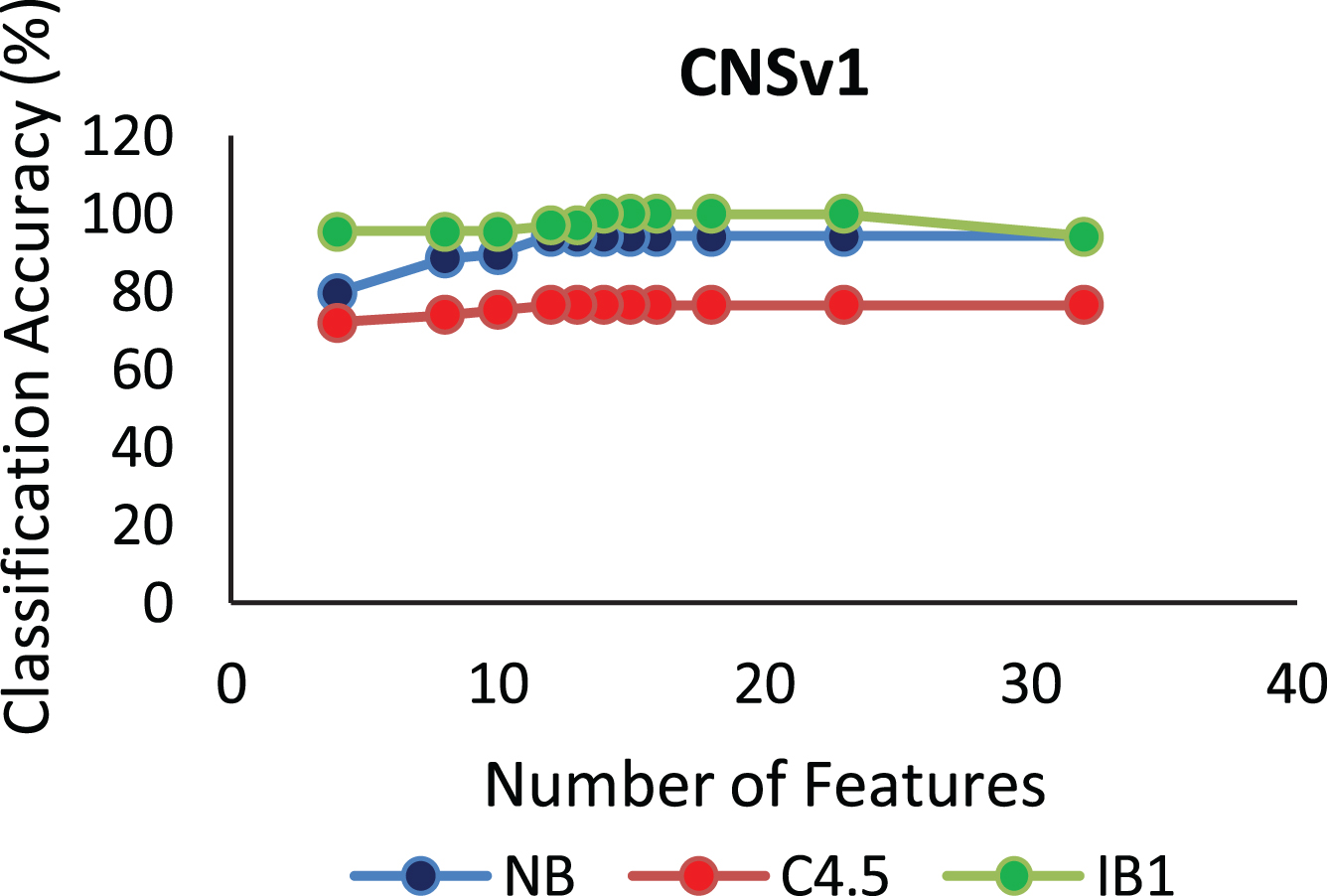
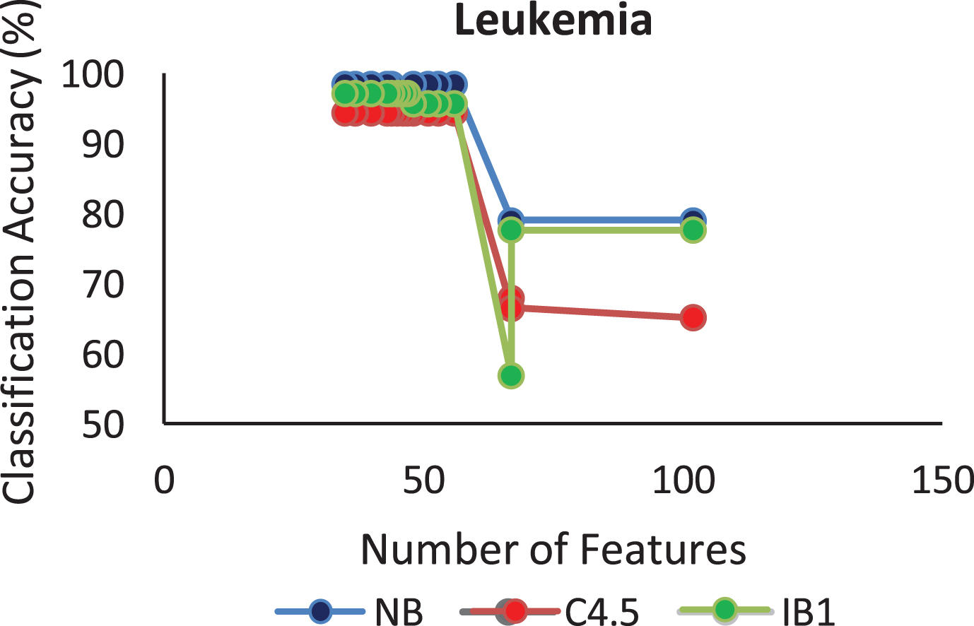
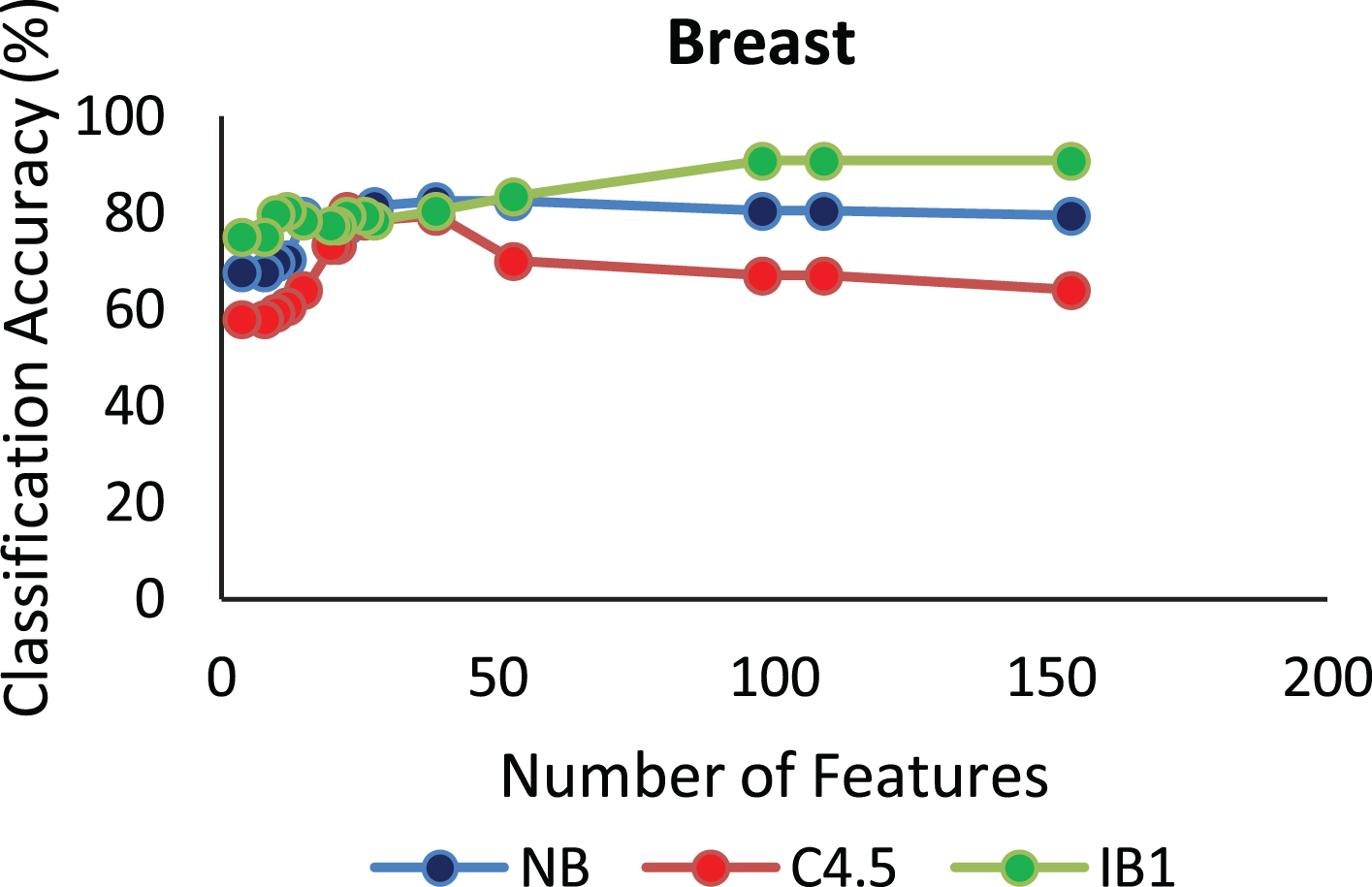
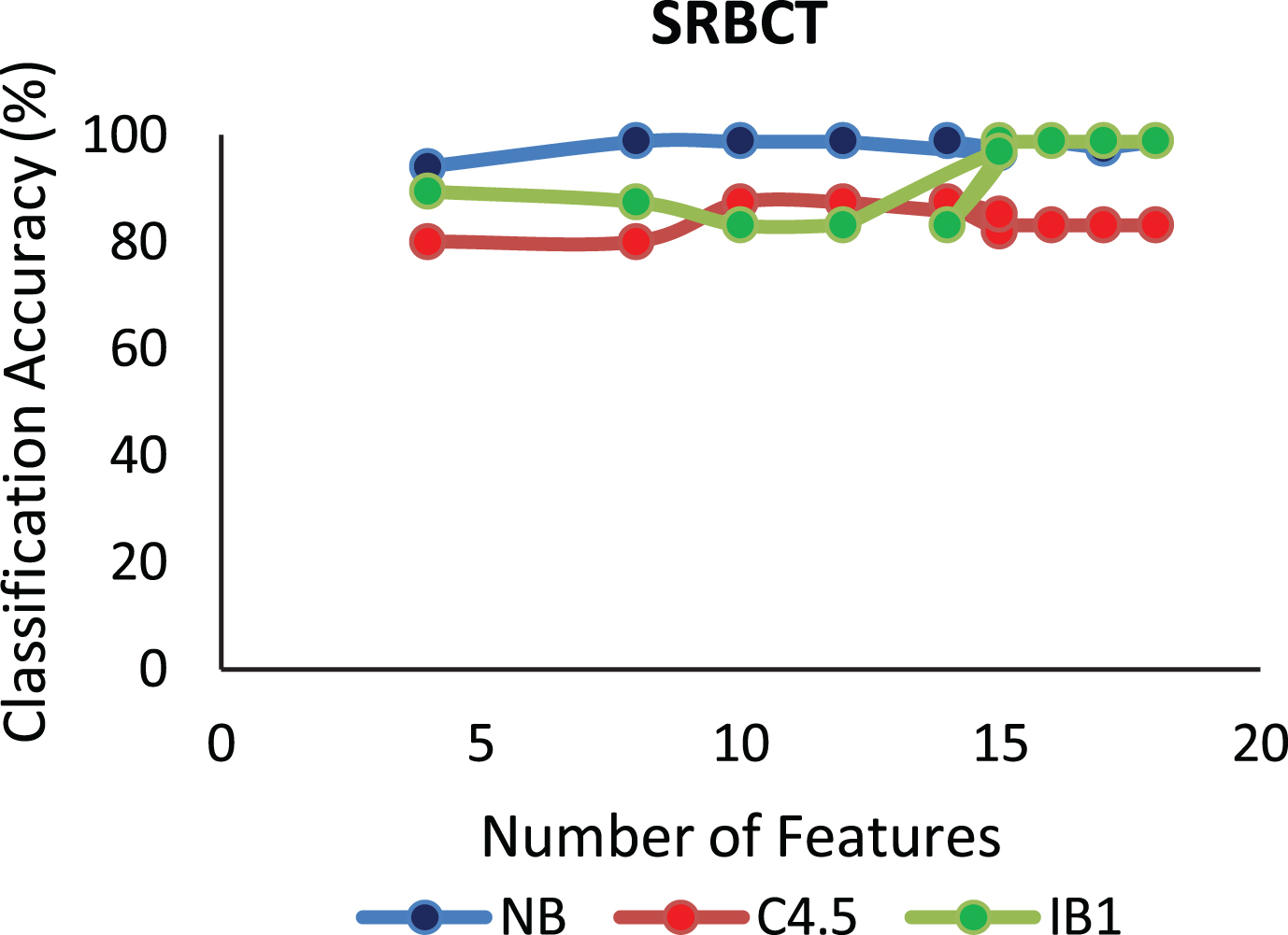
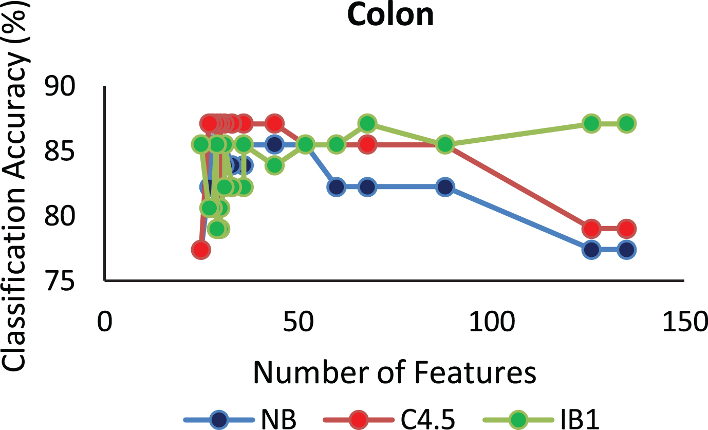
The analysis from Figs. 1–9 shows that initial iterations i.e. from 2 to 7, the number of features/genes selected is high in number with a good accuracy. As the iterations keep on increasing, number of features keeps on decreasing with some increase in accuracy. Further increasing the number of iterations decreases the number of genes and decreases the classification accuracy. Therefore, it is observed that the number of iterations should not be very high nor very low. For instance, in case of Fig. 1, for Colon_1 dataset, when ‘numIter’ is from 8 to 20, number of genes becomes constant with approximately similar accuracy values. Below this range, the numbers of genes are very large and above this range, the number of genes decreases along with a gradual decrease in accuracies. Therefore, the maximum accuracy of 100 percent is achieved when number the feature is 20. In case of SRBCT data, Fig. 7, when the number of features is between 15 to 20 Naïve Bayes and IB1 classifier are showing accuracy above 95 percent when ‘numIter’ is between 5 to 15.

5. Significance testing and validation

The purpose of significance testing is to provide a surety that the significant difference exists between the two techniques. It helps to determine whether there is enough evidence to reject a hypothesis about the difference in algorithms. To statistically validate whether the proposed algorithm outperforms other feature selection algorithms based on classification accuracy, a statistical test is performed named Friedman test [13].

5.1. Friedman test

The Friedman test is a non-parametric test. It is used to test for differences between ‘k’ algorithms over ‘d’ datasets. If the value of ‘k’ is greater than 5 then level of significance or rank of the algorithm can be approximated by test statistics using χ² distribution table. If there are more than two algorithms, then it is calculated as given in Equation 6. It treats the data as d*k matrix where d is number of datasets called blocks and k is number of columns, which has different algorithms. $M = \frac{12}{dk (k + 1)} \times \sum R_{j}^{2} - 3 d (k + 1)$ (4)

Where, $R_{j}^{2}$ is the square of the sum of ranks for group j, d = number of datasets, k = number of algorithms.

The null hypothesis, H₀ states that there is no significant difference between the feature selection algorithms based on accuracies for all three classifiers. Decision rule rejects the null hypothesis H₀ if M > critical value. value. In case of Hypothesis rejection posthoc based Nemenyi test [36] is applied in order to compare the performance.

Nemenyi test says that there is no performance difference between the two algorithms if the corresponding average ranks (Rx-Ry where Rx and Ry are the average ranks of algorithms x and y respectively) differ by more than the critical difference (CD). $CD = q_{\infty} \sqrt{\frac{k (k + 1)}{6 N}}$ (5)

Where, k is number of algorithms, N is number of datasets and q_∞ is based on the Studentized range statistic divided by $\sqrt{2}$ .

Therefore, this paper has performed three Friedman tests to explore the classification accuracies found from each of the three classifiers. As the dataset used here are 10 in number, the value of parameter d = 10, Number of algorithms k = 5 and critical value is taken as ∞=1%. The Friedman test gives the rank Rj as 48,32,30,18.5,17 for five algorithms with p = 0.0002 when compared with the accuracies calculated using Naïve Bayes Classifier. The p value is sufficiently small to provide evidence against H0. The null hypothesis is rejected in each test and we can say that all feature selection algorithms are performing differently.

Further to compare the two algorithms Nemenyi test is performed. The value of critical distance is found to be 1.229. Two classifiers are performing differently when the average rank differs at least by critical difference. Tables 4 and 5 shows the average rank difference between each of the four algorithms found in case of Naïve Bayes and IB1classifier. The proposed algorithm is statistically verified whose results are shown in Tables 4 and 5.

Table 4

Average rank difference found using Friedman test in case of Naïve Bayes Classifier

	Proposed	RFST	RF	FAST	FCBF
FCBF	3.1	2.95	1.8	1.6	0
FAST	1.5	1.35	0.2	0	1.6
RF	1.3	1.15	0	0.2	1.8
RFST	0.15	0	1.15	1.35	2.95
Proposed	0	0.15	1.3	1.5	3.1

Table 5

Average rank difference found using Friedman test in case of IB1 Classifier

	Proposed	RFST	RF	FAST	FCBF
FCBF	3.3	3.05	2.1	1.05	0
FAST	2.25	2	1.05	0	1.05
RF	1.2	0.95	0	1.05	2.1
RFST	0.25	0	0.95	2	3.05
Proposed	0	0.25	1.2	2.25	3.3

6. Conclusion

This paper proposes and implements a feature subset selection algorithm useful for microarray data. In the Algorithm 1, qualitative mutual information measure is considered to remove the irrelevant as well as the redundant features from the data. It also exhibits the robust and stable gene subset. Random Forest algorithm is implemented in between this proposed algorithm to find importance score of each feature. This importance score is utilized as it is helpful in finding the correlation as well as interaction between the features. Using this property, this paper calculates the share of preference for each variable. This share of preference has been used as utility measure along with mutual information of each variable with class/target. It also resolves the short coming of random forest by balancing each dataset before giving it as input to the Random forest algorithm. The classification results on ten microarray data shown in Table 2 depicts that the Algorithm 1 has improved the accuracy as compared to other feature selection methods for seven out of ten datasets. For two of the datasets, melanoma and leukemia the proposed RFST algorithm is performing better. Algorithm 1 is also effective in producing a reliable gene subset. One of the statistical tests named Friedman test applied on the algorithms also proves that the Algorithm 1 is significantly better than other feature selection algorithms. When Algorithm 1 is compared with latest gene selection algorithms in Table 3, it is observed that Algorithm 1 is at par with them.

References

Almuallim and

T.G.

Dietterich , Algorithms for Identifying Relevant Features, Proc Ninth Canadian Conf Artificial Intelligence, 1992, pp. 38–45.

C.J.

Alonso-González ,

Q.I.

Moro-Sancho ,

Simon-Hurtado and

Varela-Arrabal , Microarray gene expression classification with few genes: Criteria to combine attribute selection and classification methods, Expert Systems with Applications 39(8) (2012), 7270–7280.

Alshamlan ,

Badr and

Alohali , mRMR-ABC: A hybrid gene selection algorithm for cancer classification using microarray gene expression profiling, BioMed Research International (2015).

Anaissi ,

P.J.

Kennedy ,

Goyal and

D.R.

Catchpoole , A balanced iterative random forest for gene selection from microarray data, BMC Bioinformatics 14(1) (2013), (261.

Biau and

Scornet , A random forest guided tour, Test 25(2) (2016), 197–227.

Bittner ,

Meltzer ,

Chen ,

Jiang ,

Seftor ,

Hendrix ,

Radmacher ,

Simon ,

Yakhini ,

Ben-Dor and

Sampas , Molecular classification of cutaneous malignant melanoma by gene expression profiling, Nature 406(6795) (2000), 536–540.

Bolón-Canedo ,

Sánchez-Marono ,

Alonso-Betanzos ,

J.M.

Benítez and

Herrera , A review of microarray datasets and applied feature selection methods, Information Sciences 282 (2014), 111–135.

Breiman , Random forests, Machine Learning 45(1) (2001), 5–32.

Chen and

Ishwaran , Random forests for genomic data analysis, Genomics 99(6) (2012), 323–329.

10.

T.M.

Cover and

J.A.

Thomas , Elements of information theory 2nd edition, 2006.

11.

Díaz-Uriarte and

S.A.

De Andres , Gene selection and classification of microarray data using random forest, BMC bioinformatics 7(1) (2006), (1.

12.

E.R.

Dougherty , Small sample issues for microarray-based classification, International Journal of Genomics 2(1) (2001), 28–34. A review of microarray datasets and applied feature selection methods.

13.

Friedman , A comparison of alternative tests of significance for the problem of m ranking, Annals of Math Statistics 11 (1940), 86–92.

14.

Genuer ,

J.M.

Poggi and

Tuleau-Malot , VSURF: An r package for variable selection using random forests, The R Journal 7(2) (2015), 19–33.

15.

Guyon and

Elisseeff , An introduction to variable and feature selection, Journal of Machine Learning Research (3) (2003), 1157–1182.

16.

M.A.

Hall , Correlation-Based Feature Selection for Discrete and Numeric Class Machine Learning, In: Proceedings of 17th International Conference on Machine Learning, 2000, pp. 359–366.

17.

Hoque ,

D.K.

Bhattacharyya and

J.K.

Kalita , MIFS-ND: A mutual information-based feature selection method, Expert Systems with Applications 41(14) (2014), 6371–6385.

18.

Huang ,

Cai and

Xu , A filter approach to feature selection based on mutual information, In Cognitive Informatics, 2006 ICCI 2006 5th IEEE International Conference on, Vol. 1, 2006, pp. 84–89. IEEE.

19.

Irgon ,

C.C.

Huang ,

Zhang ,

Talantov ,

Bhanot and

Szalma , Robust multi-tissue gene panel for cancer detection, BMC Cancer 10(1) (2010), (1.

20.

Khan ,

Wei ,

Ringner ,

L.H.

Saal ,

Ladanyi and

Westermann , Classification and diagnosis prediction of cancers using gene expression profiling and artificial neural networks, Nat Med 7 (2001), 673–679.

21.

Jain and

Zongker , Feature selection: Evaluation, application, and small sample performance, IEEE Transactions on Pattern Analysis and Machine Intelligence 19(2) (1997), 153–158.

22.

Jain and

C.A.

Murthy , A new estimate of mutual information based measure of dependence between two variables: Properties and fast implementation, International Journal of Machine Learning and Cybernetics 7(5) (2016), 857–875.

23.

Yang ,

Cai , et al., A stable gene selection in microarray data analysis, BMC Bioinformatics 228 (2006), 7.

24.

Kira and

L.A.

Rendell , The Feature Selection Problem: Traditional Methods and a New Algorithm, Proc 10th National Conference Artificial Intelligence, 1992, pp. 129–134.

25.

Kohavi and

G.H.

John , Wrapper for feature subset selection, Artificial Intelligence 97(1) (1997), 273–324.

26.

Kononenko and Estimating, Attributes: Analysis and Extensions of RELIEF, Proceedings of European Conference Machine Learning, 1994, pp. 171–182.

27.

Laiho ,

Kokko ,

Vanharanta ,

Salovaara ,

Sammalkorpi ,

Järvinen ,

J.P.

Mecklin ,

T.J.

Karttunen ,

Tuppurainen ,

Davalos and

Schwartz , Serrated carcinomas form a subclass of colorectal cancer with distinct molecular basis, Oncogene 26(2) (2007), 312–320.

28.

Yu ,

Huan ,

Yu and

Liu , Feature selection for high-dimensional data: A fast correlation-based filter solution, In ICML Washington DC 20(2) (2003), 856-863.

29.

Luan ,

Qi and

Shen , Multi-modal image registration by quantitative-qualitative measure of mutual information (q-mi), In International Workshop on Computer Vision for Biomedical Image Applications, Springer Berlin Heidelberg, 2005, pp. 378–387.

30.

Ma and

Fan , CURE-SMOTE algorithm and hybrid algorithm for feature selection and parameter optimization based on random forests, BMC Bioinformatics 18(1) (2017), (169.

31.

Mahmoud ,

Harrison ,

Perperoglou ,

Gul ,

Khan ,

M.V.

Metodiev and

Lausen , A feature selection method for classification within functional genomics experiments based on the proportional overlapping score, BMC Bioinformatics 15(1) (2014), (274.

32.

Mimaroglu and

Aksehirli , Diclens: Divisive clustering ensemble with automatic cluster number, IEEE/ACM Transactions on Computational Biology and Bioinformatics 9(2) (2012), 408–420.

33.

Atiyeh and

M.H.

Moattar , Robust feature selection from microarray data based on cooperative game theory and qualitative mutual information, Advances in Bioinformatics 2016 (2016).

34.

Nagpal and

Singh , Identification of significant features using random forest for high dimensional microarray data, Journal of Engineering Science and Technology 13(8) (2018), 2446–2463.

35.

Nagpal and

Singh , A feature selection algorithm based on qualitative mutual information for cancer microarray data, Procedia Computer Science 132 (2018), 244–252.

36.

Nemenyi , Distribution-Free Multiple Comparison, PhD thesis, Princeton Univ, 1963.

37.

U.B.

Neto , Fads and fallacies in the name of small-sample microarray classification-A highlight of misunderstanding and erroneous usage in the applications of genomic signal processing, IEEE Signal Processing Magazine 24(1) (2007), 91–99.

38.

S.L.

Pomeroy ,

Tamayo ,

Gaasenbeek ,

L.M.

Sturla ,

Angelo ,

M.E.

McLaughlin ,

J.Y.

Kim ,

L.C.

Goumnerova ,

P.M.

Black ,

Lau and

J.C.

Allen , Prediction of central nervous system embryonal tumour outcome based on gene expression, Nature 415(6870) (2002), 436–442.

39.

Qi ,

Sun ,

Sun and

Pan , Ranking analysis for identifying differentially expressed genes, Genomics 97(5) (2011), 326–329.

40.

Ridge , Kent Ridge Bio-medical Dataset http://datam.i2r.a-star.edu.sg/datasets/krbd/, 2009.

41.

J.I.

Risinger ,

G.L.

Maxwell ,

G.V.R.

Chandramouli ,

Jazaeri ,

Aprelikova ,

Patterson ,

Berchuck and

J.C.

Barrett , Microarray analysis reveals distinct gene expression profiles among different histologic types of endometrial cancer, Cancer Research 63(1) (2003), 6–11.

42.

D.A.

Salem ,

Seoud ,

Ahmed and

H.A.

Ali , Mgs-cm: A multiple scoring gene selection technique for cancer classification using microarrays, International Journal of Computer Applications 36(6) (2011), 30–37.

43.

Song ,

Ni and

Wang , A fast clustering-based feature subset selection algorithm for high-dimensional data, IEEE Transactions on Knowledge and Data Engineering 25(1) (2013), 1–14.

44.

C.D.A.

Vanitha ,

Devaraj and

Venkatesulu , Gene expression data classification using support vector machine and mutual information-based gene selection, Procedia Computer Science 47 (2015), 13–21.

45.

Zhang ,

Yang ,

C.Y.

Xiong ,

Zhou and

Zhang , Feature selection for classification with class-separability strategy and data envelopment analysis Neurocomputing, 166 (2015), 172–184.

46.

J.G.

Zhang and

H.W.

Deng , Gene selection for classification of microarray data based on the Bayes error, BMC Bioinformatics 8(1) (2007), 370.