Bounded lattice fuzzy coincidence theorems with applications

Abstract

The main focus of the present paper is to establish a common coincidence point theorem for a pair of L-fuzzy mappings and a non-fuzzy mapping under a generalized φ-contractive condition on a metric space in association with the Hausdorff distance on a class of L-fuzzy sets. A generalized common coincidence point theorem with the $d_{L}^{\infty}$ metric on 1- cuts of L-fuzzy sets is also obtained, which generalizes many recent results in literature. As applications, an analogous coincidence point theorem for crisp mappings is achieved to study some existence theorems of solution for a class of nonlinear integral equations. Even as direct application of coincidence of L- fuzzy mappings, an implicit function theorem is established which can be used to find an explicit restriction of a given implicit relation. For verification and elaboration of our results some interesting and non-trivial examples are presented as well.

Keywords

Coincidence point implicit function theorem integral equation

1 Introduction

In our daily life, problems in economics, engineering, social sciences, and medical sciences do not always involve crisp data. Traditional mathematical methods cannot be frequently used because a large number of uncertainties exists in these practical problems. To overwhelmed these reservations, concepts like fuzzy set, intuitionistic fuzzy set, soft set, rough set, and bipolar fuzzy set have been prepared (see [18 , 35]). Scholars should continue to explore the abstract algebraic concepts and results in the wider context of the fuzzy setting. One structure that’s mathematical applications are most generally argued is lattice theory. In an extensive variety of mathematical problems, the existence of a solution is corresponding to the existence of a fixed point for an appropriate map. The theory of fixed points has been evolved as an active and very useful area of research due to its applications in mathematics and related disciplines. The fixed point theorem based on the contraction principle is applied usually in proving the existence and uniqueness of the solutions of some scalar and mainly functional equations (for example differential and integral equations). In brief, fixed point theory is a powerful tool to determine uniqueness of solutions to dynamical systems and is widely used in theoretical and applied analysis. One such application is to feasibility and inverse optimization problems arising in the context of finding good radiation dose plans for the cure of cancer. These problems can often be formulated as inverse or feasibility problems, for which fixed-point theory provides algorithms, or arguments for the convergence of various iterative methods.

Fuzzy sets were introduced by Zadeh [33] in 1965 to represent/manipulate data and information possessing nonstatistical uncertainties. It was specifically designed to represent uncertainty and vagueness and to provide formalized tools for dealing with the imprecision intrinsic to many problems. Later in 1967, Goguen [14] extended this idea to L-fuzzy set theory by replacing the interval [0, 1] with a completely distributive lattice L. Ma et al. [18, 19] did a survey of decision making methods based on certain hybrid soft set models and two classes of hybrid soft set models. Since the concept of distance function plays an important role in approximation theory, therefore fuzzy sets and L-fuzzy sets have further been applied to the classical notion of metric.

In continuation of many investigations in fixed point theory, Abu-Donia [1], established common fixed points theorems for fuzzy mappings in metric spaces under φ contraction condition and Shatanawi [26] obtained some fixed point results for generalized ψ-weak contraction mappings in orbitally metric spaces. Azam et al. [5] established common fixed point of fuzzy mappings under a contraction condition. Tripathy et al. [31] proved a fixed point theorem in a generalized fuzzy metric space. Tripathy et al. [28 –30] also has done work on convergence of series of fuzzy real number, fixed point results in fuzzy 2-metric spaces, fixed and periodic point theorems in fuzzy metric spaces. Das [12] established and proved theorems on fuzzy normed linear space valued statistically convergent sequences. In 1981, Heilpern [13] gave a fuzzy extension of Banach contraction principle and Nadler [20] fixed point theorems by introducing the concept of fuzzy contraction mappings in connection with d_∞-metric for fuzzy sets. Subsequently several other authors (e.g., [6–11 , 27]) generalized this result and studied the existence of fixed points and common fixed points of fuzzy approximate quantity-valued mappings satisfying a contractive type condition in metric linear spaces. Recently Kamran [16] Azam et al. [4 , 11] and some other authors (e.g., [15, 17]) continue to study fixed points of fuzzy set valued mappings in connection with d_∞-metric and Hausdorff metric for fuzzy subsets. Zhou et al. [41] worked on properties of the cut-sets of intuitionistic fuzzy relations.

Hausdorff distance for α-cut sets of L-fuzzy mapps was introduced by Rashid et al. [23, 24], to study fixed point theorems for L-fuzzy set valued-mappings and coincidence theorems for a crisp mapping and a sequence of L-fuzzy mappings. Many researchers have studied fixed point theory in the fuzzy context of metric spaces and normed spaces. Recently, Rashid et al. [25] established fixed point theorems for L-fuzzy mappings in quasi-pseudo metric spaces. Subsequently, Azam et al. [2] worked on coincidence point of L-fuzzy sets endowed with graph. In 2016, Azam et al. [3] obtained L-fuzzy fixed points in cone metric spaces.

In the present work, common coincidence point theorems for a crisp and a pair of L-fuzzy mappings satisfying generalized φ-contractive condition have been formulated and proved. A generalized common coincidence point theorem with the $d_{L}^{\infty}$ metric on 1- cuts of L-fuzzy sets is established, from which some corollaries has been deduced as well. Some applications regarding the existence of solution for non-linear integral equations and implicit function theorem of mathematical analysis have been achieved. Moreover, some interesting and non-trivial examples are presented.

2 Preliminaries

In this section, we recall the concepts and definitions related to bounded lattice, fuzzy sets, hausdorff metric spaces, metric linear spaces etc.

Let (X, d) be a metric space, C (2^X) be the family of nonempty compact subsets of X and A, B ∈ C (2^X). $\begin{matrix} d (x, A) = inf_{y \in A} d (x, y), \end{matrix}$ $\begin{matrix} d (A, B) = inf_{x \in A, y \in B} d (x, y) . \end{matrix}$ Then the Hausdorff metric H on C (2^X) induced by d is defined as: $\begin{matrix} H (A, B) = max {sup_{a \in A} d (a, B), sup_{b \in B} d (A, b)} . \end{matrix}$

For crisp subset A of X, we denote the characteristic function of by χ_A .

Definition 1. [18, 32] A fuzzy set in X is a function with domain X and values in [0, 1]. Let $F (X)$ be the collection of all fuzzy sets in X . If A is a fuzzy set and x ∈ X, then the function values A (x) is called the grade of membership of x in A.

The α -level set of a fuzzy set A, denoted by [A] _α, is defined as follows $\begin{matrix} {[A]}_{α} = {x : A (x) \geq α} if α \in (0, 1], \end{matrix}$ $\begin{matrix} {[A]}_{0} = \bar{{x : A (x) > 0},} \end{matrix}$ $\begin{matrix} \hat{A} = {x : A (x) = max_{y \in X} A (y)} . \end{matrix}$ Definition 2. A partially ordered set (L, ⪯ _L) is called a lattice; if a ∨ b ∈ L, a ∧ b ∈ L for any a, b ∈ L. A lattice L is said to be

a complete lattice; if ⋁A ∈ L, ⋀A ∈ L for any A ⊆ L,

a distributive lattice; if a ∨ (b ∧ c) = (a ∨ b) ∧ (a ∨ c), a ∧ (b ∨ c) = (a ∧ b) ∨ (a ∧ c) for any a, b, c ∈ L,

a complete distributive lattice; if a ∨ (⋀ bi) = ⋀ _i (a ∧ bi), a ∧ (⋁ _ibi) = ⋁ _i (a ∧ bi) for any a, bi ∈ L,

a bounded lattice; if it has a top element 1_L and a bottom element 0_L, which satisfy 0_L ⪯ _Lx ⪯ _L1_L for every x ∈ L.

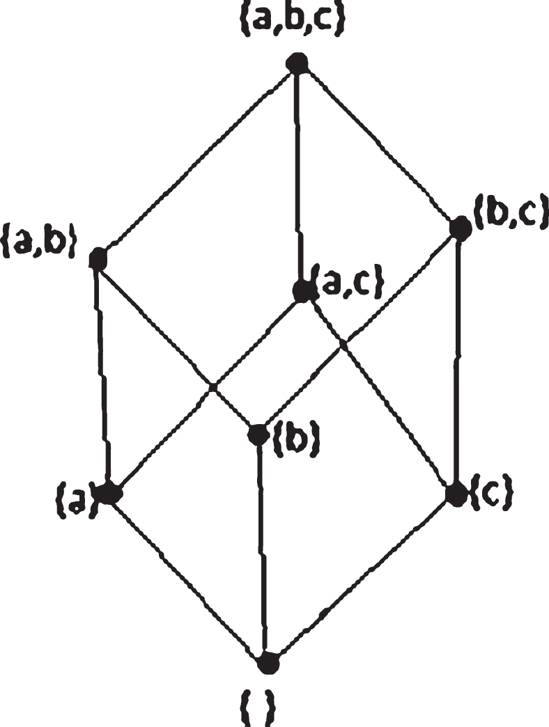
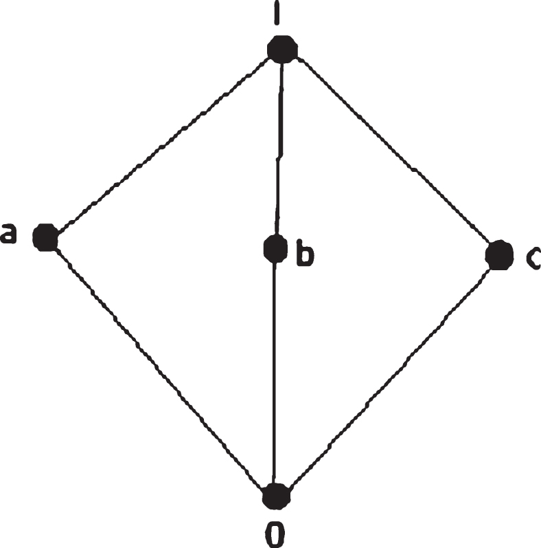
Example. Let S = {a, b, c} be an arbitrary set, then P (S)(power set of S) with partial order ⊆ shown in figure 1 is a distributive lattice. A lattice shown in figure 2 is non-distributive because a ∧ (b ∨ c) = a ∧ I = a and (a ∧ b) ∨ (a ∧ c) =0 ∨ 0 =0, i.e. distributive law does not hold.

Fig.1

Distributive Lattice.

Fig.2

Non-distributive Lattice.

Definition 3. (Goguen [14]) Let L be a lattice, the top and bottom elements of L are 1_L and 0_L respectively, and if a, b ∈ L, a ∨ b = 1_L and a ∧ b = 0_L then b is a unique complement of a denoted by $\overset{´}{a}$ .

Definition 4. [14] An L-fuzzy set in X is a function with domain X and values in L, where L is a complete distributive lattice with 1_L and 0_L, i.e if A : X → L, then A is an L-fuzzy set. $F_{L} (X)$ is the collection of all L-fuzzy sets in X . If A is an L-fuzzy set and x ∈ X, then the function values A (x) is called the grade of membership of x in A.

Remark. If L = [0, 1], then the L-fuzzy set is the special case of fuzzy sets in the original sense of Zadeh [33], which shows that the concept of L-fuzzy set is larger.

The α_L -level set of an L-fuzzy set A, denoted by [A] _{α
_L}, is defined as follows: $\begin{matrix} {[A]}_{α_{L}} = {x : α_{L} ⪯_{L} A (x)} for α_{L} \in L - {0_{L}}, \end{matrix}$ $\begin{matrix} {[A]}_{0_{L}} = \bar{{x : 0_{L} ⪯_{L} A (x)} .} \end{matrix}$

If $max_{y \in X} A (y)$ exists, then $\begin{matrix} \hat{A} = {x : A (x) = max_{y \in X} A (y)} . \end{matrix}$

An L-fuzzy set A in a metric linear space V is said to be an approximate quantity if and only if [A] _{α
_L} is compact and convex in V for each α_L ∈ L - {0_L} and $sup_{x \in V} A (x) = 1 .$

Define some sub-collections of $F_{L} (X)$ and $F_{L} (V)$ as follows: $\begin{matrix} W_{L} (V) = {A \in F_{L} (V) : \\ \times A is an approximate quantity in V}, \end{matrix}$ $\begin{matrix} K (X) = {A \in F_{L} (X) : max_{y \in X} A (y) existed, \\ \times \hat{A} \in C (2^{X})}, \end{matrix}$ $\begin{matrix} X) = {A \in F_{L} (X) : {[A]}_{α_{L}} \in C (2^{X}), \\ \times for each α_{L} \in L} . \end{matrix}$

For $A, B \in F_{L} (X),$ A ⊂ B means A (x) ⪯ _LB (x) for each x ∈ X. If there exists an α_L ∈ L - {0_L} such that [A] _{α
_L}, [B] _{α
_L} ∈ C (2^X) then define $\begin{matrix} p_{α_{L}} (A, B) & = & inf_{x \in {[A]}_{α_{L}}, y \in {[B]}_{α_{L}}} d (x, y), \\ D_{α_{L}} (A, B) & = & H ({[A]}_{α_{L}}, {[B]}_{α_{L}}) . \end{matrix}$ If [A] _{α
_L}, [B] _{α
_L} ∈ C (2^X) for each α_L ∈ L then define $p (A, B), d_{L}^{\infty} (A, B) : C_{L} (X) \times C_{L} (X) \to ℝ,$ (induced by the Hausdorff metric H) as follows: $\begin{matrix} p (A, B) & = & sup_{α_{L}} p_{α_{L}} (A, B), \\ d_{L}^{\infty} (A, B) & = & sup_{α_{L}} D_{α_{L}} (A, B) . \end{matrix}$

Definition 5. Let W be an arbitrary set, X be a metric space. A mapping T is called L-fuzzy mapping if T is a mapping from W into $F_{L} (X)$ . An L-fuzzy mapping T is an L-fuzzy subset on W × X with membership function T (x) (y). The function T (x) (y) is the grade of membership of y in T (x) . The family of all mappings from W into $F_{L} (X)$ is denoted by ${(F_{L} (X))}^{W} .$

Definition 6. Let (X, d) be a metric space and $T : X \to F_{L} (X)$ . A point z ∈ X is said to be an L-fuzzy fixed point of T if z ∈ [Tz] _{α
_L}, for some α_L ∈ L - {0_L}.

Definition 7. A point u ∈ W is called L-fuzzy coincidence point of F : W → X, T : W → $F_{L} (X)$ if F (u) ∈ [Tu] _{α
_L}. The set {u ∈ W: F (u) ∈ [Tu] _{α
_L}, α_L ∈ L - {0_L} of all coincidence points of F and T is denoted by C_(F,T) . A point x∈ C_(I,T) (where I is identity map) is a fixed point of T.

3 Bounded Lattice Fuzzy Coincidence Theorems

Lemma 1. Let A and B be nonempty closed and bounded subsets of a metric space (X, d) . If a ∈ A, then d (a, B) ≤ H (A, B) .

Lemma 2. Let (V, d_v) be a complete metric linear space, $T : V ⟶ W_{L} (V)$ be a fuzzy mapping and x₀ ∈ V . Then there exists x₁ ∈ V such that χ{x₁} ⊂ T (x₀) .

Lemma 3. Let $φ : ℝ^{+} \to ℝ^{+}$ be a nondecreasing function satisfying the following conditions:φ is continuous from right and $\sum_{i = 0}^{\infty} φ^{i} (t) < \infty$ for all t > 0 (φⁱ denote the ith iterative function of φ). Then φ (t) < t .

In the following we always assume that Δ^∗ be the set of all continuous functions satisfying the condition of Lemma 3.

Theorem 4. Let Y be a nonempty set, (X, d) be a metric space and $Φ, Ψ : Y \to F_{L} (X), F : Y \to X$ . Suppose that for x ∈ Y there exists α_{Φ_L(x)}, α_{Ψ_L(x)} ∈ L - {0_L} such that [Φx] _{α
_{Φ_L(x)}}, [Ψx] _{α
_{Ψ_L(x)}} ∈ C (2^X) , $(1) ⋃_{x \in Y} [[Φ x]_{α_{Φ_{L} (x)}} \cup [Ψ x]_{α_{Ψ_{L} (x)}}] \subseteq FY .$ (1) Suppose that there exists φ ∈ Δ^∗ such that for all x, y ∈ Y

$\begin{matrix} (2) & H ([Φ x]_{α_{Φ_{L} (x)}}, [Ψ x]_{α_{Ψ_{L} (x)}}) \leq φ (max {d (Fx, Fy), \\ d (Fx, [Φ x]_{α_{Φ_{L} (x)}}), d (Fy, [Ψ x]_{α_{Ψ_{L} (x)}}), \\ \frac{1}{2} [d (Fx, [Ψ x]_{α_{Ψ_{L} (x)}}) + d (Fy, [Φ x]_{α_{Φ_{L} (x)}})]}) . \end{matrix}$ (2)

If F is injective and either FY or ⋃ _x∈Y [[Φx] _{α
_{Φ_L(x)}} ∪ [Ψx] _{α
_{Ψ_L(x)}}] is complete. Then $\begin{matrix} C_{(F, Φ)} ⋂ C_{(F, Ψ)} \neq φ . \end{matrix}$ Moreover, if [Φx] _{α
_{Φ_L(x)}}, [Ψx] _{α
_{Ψ_L(x)}} are singleton subsets of X for all x, y ∈ X, then C_(F,Φ) ⋂ C_(F,Ψ) is singleton.

Proof. Choose x₀ ∈ Y, then by hypotheses [Φx₀] _{α
_{Φ_L(x₀)}} ∈ C (2^X) . Using (1) and the compactness of [Φx₀] _{α
_{Φ_L(x₀)}}, we obtain x₁ ∈ Y such that Fx₁ ∈ [Φx₀] _{α
_{Φ_L(x₀)}} and $\begin{matrix} d ({Fx}_{0}, {Fx}_{1}) = d ({Fx}_{0}, [Φ x_{0}]_{α_{Φ_{L} (x_{0})}}) . \end{matrix}$

Similarly, we can choose x₂ ∈ Y such that Fx₂ ∈ [Ψx₁] _{α
_{Ψ_L(x₁)}} and $\begin{matrix} d ({Fx}_{1}, {Fx}_{2}) = d ({Fx}_{1}, [Ψ x_{1}]_{α_{Ψ_{L} (x_{1})}}) . \end{matrix}$

By induction we produce sequences {x_n } and { Fx_n } of points of Y and FY respectively such that $\begin{matrix} {Fx}_{2 k + 1} \in [Φ x_{2 k}]_{α_{Φ_{L} (x_{2 k})}}, \end{matrix}$ $\begin{matrix} {Fx}_{2 k + 2} \in [Ψ x_{2 k + 1}]_{α_{Ψ_{L} (x_{2 k + 1})}}, \end{matrix}$ k = 0, 1, 2, ⋯ such that $\begin{matrix} d ({Fx}_{2 k}, {Fx}_{2 k + 1}) = d ({Fx}_{2 k}, [Φ x_{2 k}]_{α_{Φ_{L} (x_{2 k})}}), \end{matrix}$ $\begin{matrix} d ({Fx}_{2 k + 1}, {Fx}_{2 k + 2}) & = & d ({Fx}_{2 k + 1}, \\ \times [Ψ x_{2 k + 1}]_{α_{Ψ_{L} (x_{2 k + 1})}}), \end{matrix}$ k = 0, 1, 2, ⋯ .

Using Lemma 1 along with the above equations, we have $\begin{matrix} d ({Fx}_{2 k}, {Fx}_{2 k + 1}) \leq H ([Ψ x_{2 k - 1}]_{α_{Ψ_{L} (x_{2 k - 1})}}, \\ [Φ x_{2 k}]_{α_{Φ_{L} (x_{2 k})}}), \end{matrix}$ $\begin{matrix} d ({Fx}_{2 k + 1}, {Fx}_{2 k + 2}) \leq H ([Φ x_{2 k}]_{α_{Φ_{L} (x_{2 k})}}, \\ [Ψ x_{2 k + 1}]_{α_{Ψ_{L} (x_{2 k + 1})}}), \end{matrix}$ where k = 0, 1, 2, ⋯ .

Assume that Fx_2k = Fx_2k+1 for some k ≥ 0, then as F is injective, $\begin{matrix} x_{2 k} = x_{2 k + 1}, \end{matrix}$ $\begin{matrix} [Ψ x_{2 k}]_{α_{Ψ_{L} (x_{2 k})}} = [Ψ x_{2 k + 1}]_{α_{Ψ_{L} (x_{2 k + 1})}} \end{matrix}$ and $\begin{matrix} d ({Fx}_{2 k + 1}, {Fx}_{2 k + 2}) \leq H ([Φ x_{2 k}]_{α_{Φ_{L} (x_{2 k})}}, \\ [Ψ x_{2 k + 1}]_{α_{Ψ_{L} (x_{2 k + 1})}}) \\ \leq φ (max {d ({Fx}_{2 k}, {Fx}_{2 k + 1}), \\ d ({Fx}_{2 k}, [Φ x_{2 k}]_{α_{Φ_{L} (x_{2 k})}}), \\ d ({Fx}_{2 k + 1}, [Ψ x_{2 k + 1}]_{α_{Ψ_{L} (x_{2 k + 1})}}), \\ \frac{1}{2} [d ({Fx}_{2 k}, [Ψ x_{2 k + 1}]_{α_{Ψ_{L} (x_{2 k + 1})}}) \\ + d ({Fx}_{2 k + 1}, [Φ x_{2 k}]_{α_{Φ_{L} (x_{2 k})}})]}) \\ \leq φ (max {d ({Fx}_{2 k + 1}, {Fx}_{2 k + 2}), \\ \frac{1}{2} [d ({Fx}_{2 k}, {Fx}_{2 k + 2}) + d ({Fx}_{2 k + 1}, {Fx}_{2 k + 1})]}) \\ \leq φ (d ({Fx}_{2 k + 1}, {Fx}_{2 k + 2})) . \end{matrix}$

Since, φ (t) < t for all t > 0, therefore, the above inequality implies that d (Fx_2k+1, Fx_2k+2) = 0, which further implies thatFx_2k = Fx_2k+1 ∈ [Φx_2k] _{α
_{Φ_L(x_2k)}}, $\begin{matrix} {Fx}_{2 k} & = & {Fx}_{2 k + 1} = {Fx}_{2 k + 2} \in [Ψ x_{2 k + 1}]_{α_{Ψ_{L} (x_{2 k + 1})}} \\ = & [Ψ x_{2 k}]_{α_{Ψ_{L} (x_{2 k})}} . \end{matrix}$

It follows that $\begin{matrix} {Fx}_{2 k} \in [Φ x_{2 k}]_{α_{Φ_{L} (x_{2 k})}} \cap [Ψ x_{2 k}]_{α_{Ψ_{L} (x_{2 k})}} . \end{matrix}$ Then we get the required result. Thus in this sequel of the proof we can suppose that Fx_n+1 ≠ Fx_n for n = 0, 1, 2 ⋯ . Again by using inequality(2), we have $\begin{matrix} d ({Fx}_{2 k + 1}, {Fx}_{2 k + 2}) \leq H ([Φ x_{2 k}]_{α_{Φ_{L} (x_{2 k})}}, \\ [Ψ x_{2 k + 1}]_{α_{Ψ_{L} (x_{2 k + 1})}}) \\ \leq φ (max {d ({Fx}_{2 k}, {Fx}_{2 k + 1}), d ({Fx}_{2 k + 1}, {Fx}_{2 k + 2}), \\ \frac{1}{2} [d ({Fx}_{2 k}, {Fx}_{2 k + 2}) + d ({Fx}_{2 k + 1}, {Fx}_{2 k + 1})]}) \\ \leq φ (max {d ({Fx}_{2 k}, {Fx}_{2 k + 1}), d ({Fx}_{2 k + 1}, {Fx}_{2 k + 2})}) . \end{matrix}$

If $\begin{matrix} max {d ({Fx}_{2 k}, {Fx}_{2 k + 1}), d ({Fx}_{2 k + 1}, {Fx}_{2 k + 2})} \\ = d ({Fx}_{2 k + 1}, {Fx}_{2 k + 2}), \end{matrix}$ then the above inequality implies that which is a contradiction as Fx_n+1 ≠ Fx_n for n = 0, 1, 2 ⋯ , . It follows that $\begin{matrix} max {d ({Fx}_{2 k}, {Fx}_{2 k + 1}), d ({Fx}_{2 k + 1}, {Fx}_{2 k + 2})} \\ = d ({Fx}_{2 k}, {Fx}_{2 k + 1}) . \end{matrix}$

It further implies that $\begin{matrix} d ({Fx}_{2 k + 1}, {Fx}_{2 k + 2}) \leq φ (d ({Fx}_{2 k}, {Fx}_{2 k + 1})) . \end{matrix}$

Consequently, $\begin{matrix} d ({Fx}_{n + 1}, {Fx}_{n}) \leq φ (d ({Fx}_{n}, {Fx}_{n - 1})) \\ \leq φ^{2} (d ({Fx}_{n - 1}, {Fx}_{n - 2})) \\ \leq \dots \leq φ^{n} (d ({Fx}_{1}, {Fx}_{0})), \end{matrix}$ for each n ≥ 1 . Now for each positive integer m and n (n > m) , we have $\begin{matrix} d ({Fx}_{m}, {Fx}_{n}) \leq d ({Fx}_{m}, {Fx}_{m + 1}) \\ + d ({Fx}_{m + 1}, {Fx}_{m + 2}) + \dots + d ({Fx}_{n - 1}, {Fx}_{n}) \\ \leq φ^{m} (d ({Fx}_{1}, {Fx}_{0})) + φ^{m + 1} (d ({Fx}_{1}, {Fx}_{0})) \\ + \dots + φ^{n - 1} (d ({Fx}_{1}, {Fx}_{0})) \\ \leq \sum_{i = m}^{n - 1} φ^{i} (d ({Fx}_{1}, {Fx}_{0})) \leq \sum_{i = m}^{\infty} φ^{i} (d ({Fx}_{1}, {Fx}_{0})) . \end{matrix}$

Since, $\sum_{i = 1}^{\infty} φ^{i} (t) < 1$ for each t > 0 . It yields that {Fx_n} is a Cauchy sequence. As FY is complete, there exists u ∈ Y such that Fx_n → Fu (this holds also if ⋃_x∈Y [[Φx] _{α
_{Φ_L(x)}} ∪ [Ψx] _{α
_{Psi_L(x)}}] is complete with $lim_{n \to \infty} {Fx}_{n} \in ⋃_{x \in Y} [[Φ x]_{α_{Φ_{L} (x)}} \cup [Ψ x]_{α_{Ψ_{L} (x)}}] \subseteq FY$ ).

Now, Lemma 1 implies that $\begin{matrix} d (Fu, [Φ u]_{α_{Φ_{L} (u)}}) \\ \leq d (Fu, {Fx}_{2 n}) + d ({Fx}_{2 n}, [Φ u]_{α_{Φ_{L} (u)}}) \\ d (Fu, {Fx}_{2 n}) + H ([Ψ x_{2 n - 1}]_{α_{Ψ_{L} (x_{2 n - 1})}}, [Φ u]_{α_{Φ_{L} (u)}}) \\ d (Fu, {Fx}_{2 n}) + φ (max {d (Fu, {Fx}_{2 n - 1}), \\ d (Fu, [Φ u]_{α_{Φ_{L} (u)}}), d ({Fx}_{2 n - 1}, [Ψ x_{2 n - 1}]_{α_{Ψ_{L} (x_{2 n - 1})}}), \\ d (Fu, [Ψ x_{2 n - 1}]_{α_{Ψ_{L} (x_{2 n - 1})}}) + d ({Fx}_{2 n - 1}, [Φ u]_{α_{Φ_{L} (u)}})]}) \\ d (Fu, {Fx}_{2 n}) + φ (max {d (Fu, {Fx}_{2 n - 1}), \\ d (Fu, [Φ u]_{α_{Φ_{L} (u)}}), d ({Fx}_{2 n - 1}, {Fx}_{2 n}), \\ d (Fu, {Fx}_{2 n}) + d ({Fx}_{2 n - 1}, [Φ u]_{α_{Φ_{L} (u)}})]}) . \end{matrix}$ Letting n → ∞ , and using the fact that φ is continuous, we have, $\begin{matrix} d (Fu, [Φ u]_{α_{Φ_{L} (u)}}) \leq φ (d (Fu, [Φ u]_{α_{Φ_{L} (u)}}) . \end{matrix}$ Using the above inequality, we have $\begin{matrix} F (u) \in [Φ u]_{α_{Φ_{L} (u)}}, \end{matrix}$ for all x ∈ Y . Similarly, by using $\begin{matrix} d (Fu, [Ψ u]_{α_{Ψ_{L} (u)}}) \leq d (Fu, x_{2 n + 1}) \\ [Ψ u]_{α_{Ψ_{L} (u)}}), \end{matrix}$ we have $\begin{matrix} F (u) \in [Ψ u]_{α_{Ψ_{L} (u)}}, \end{matrix}$ for all x ∈ Y . Hence u ∈ (C_(F,Φ) ⋂ C_(F,Ψ)) . Finally, we show that, if [Φx] _{α
_{Φ_L(x)}}, [Ψy] _{α
_{Ψ_L(y)}} are singleton subsets of X for all x, y ∈ X, then (C_(F,Φ) ⋂ C_(F,Ψ)) is singleton. For this, assume that there exists two distinct points u, v ∈ (C_(F,Φ) ⋂ C_(F,Ψ)) . It follows that $\begin{matrix} Fu \neq Fv, \end{matrix}$ $\begin{matrix} Fu \in [Φ u]_{α_{Φ_{L} (u)}} = [Ψ u]_{α_{Ψ_{L} (u)}} \end{matrix}$ $\begin{matrix} and Fv \in [Φ v]_{α_{Φ_{L} (v)}} = [Ψ v]_{α_{Ψ_{L} (v)}} . \end{matrix}$

Using inequality (2), we obtain $\begin{matrix} d (Fu, Fv) = H ([Φ u]_{α_{Φ_{L} (u)}}, [Ψ v]_{α_{Ψ_{L} (v)}}) \\ \leq φ (max {d (Fu, Fv), d (Fu, [Φ u]_{α_{Φ_{L} (u)}}), \\ d (Fv, [Ψ v]_{α_{Ψ_{L} (v)}}), \frac{1}{2} [d (Fu, [Ψ v]_{α_{Ψ_{L} (v)}}) \\ + d (Fv, [Φ u]_{α_{Φ_{L} (u)}})]}) \\ \leq φ (max {d (Fu, Fv), d (Fu, Fu), \\ d (Fv, Fv), \frac{1}{2} [d (Fu, Fv) + d (Fv, Fu)]}) \\ \leq φ (d (Fu, Fv)) < d (Fu, Fv), \end{matrix}$ which is a contradiction, hence d (Fu, Fv) =0 and so u = v .

Next we furnish an example to support our result. For convenience, we use the following notations.

Let L be a complete bounded distributive lattice. Define a generalized characteristic function $Ω_{W_{α}^{β}} : X \to L$ of a crisp set W as $\begin{matrix} Ω_{W_{α}^{β}} (x) = {\begin{matrix} α & if x \in W \\ β & if x \notin W . \end{matrix} \end{matrix}$

Note that if L = {0, 1} and α = 1, β = 0 then $Ω_{W_{α}^{β}} = χ_{W}$ (Characteristic function of W).

Example 5. Let X = [0, ∞) , d (μ, ν) = |μ - ν|. Let L = {η, β, γ, δ} with η ⪯ _Lβ ⪯ _Lδ and η ⪯ _Lγ ⪯ _Lδ, where β and γ are not comparable, then (L, ⪯ _L) is a complete distributive Lattice. Define a pair of mappings $P, Q : (0 \infty) \to F_{L} (X)$ as follows: $\begin{matrix} P (μ) (t) = {\begin{matrix} γ & if 0 \leq t \leq 3 μ - \frac{9 μ^{2}}{2} \\ β & if 3 μ - \frac{9 μ^{2}}{2} < 3 μ \\ δ & if 3 μ < t < 6 μ \\ η & if 6 μ \leq t < \infty, \end{matrix} \end{matrix}$ $\begin{matrix} Q (μ) (t) = {\begin{matrix} δ & if 0 \leq t \leq 3 μ - \frac{9 μ^{2}}{2} \\ γ & if 3 μ - \frac{9 μ^{2}}{2} < t \leq 6 μ \\ η & if 6 μ < t < 9 μ \\ β & if 9 μ \leq t < \infty . \end{matrix} \end{matrix}$ Now define $Φ, Ψ : X ⟶ F_{L} (X)$ , F : X → X as follows: $\begin{matrix} Φ (μ) (t) = {\begin{matrix} Ω_{{0}_{η}^{δ}} & if μ = 0 \\ P (μ) & if μ \in (0, \frac{1}{3}) \\ Ω_{{\frac{1}{2}}_{η}^{δ}} & if μ > \frac{1}{3} \end{matrix} \end{matrix}$ $\begin{matrix} Ψ (μ) (t) = {\begin{matrix} Ω_{{0}_{η}^{δ}} & if μ = 0 \\ Q (μ) & if μ \in (0, \frac{1}{3}] \\ Ω_{{\frac{1}{2}}_{η}^{δ}} & if μ > \frac{1}{3}, \end{matrix} \end{matrix}$ $\begin{matrix} F μ = 3 μ for all μ \in X . \end{matrix}$ Define φ : [0, ∞) → [0, ∞) as follows: $\begin{matrix} φ (t) = {\begin{matrix} t - \frac{t^{2}}{2} & if t \in [0, 1] \\ \frac{1}{2} & if t > 1 . \end{matrix} \end{matrix}$ It is obvious that φ (t) < t for t > 0, and for μ ∈ X, if α_{Φ_L(μ)} = γ ∈ L - {0_L} and α_{Ψ_L(μ)} = δ ∈ L - {0_L}, then [Φμ] _γ, [Ψμ] _δ are compact.

If μ = ν = 0 or $μ, ν > \frac{1}{3},$ then [Φμ] _γ = [Ψμ] _δ and $\begin{matrix} H ([Φ μ]_{γ}, [Ψ ν]_{δ}) = 0 . \end{matrix}$ If $μ = 0, ν \in (0, \frac{1}{3}],$ then [Φ (0)] _γ ={ 0 }, $[Ψ ν]_{δ} = [0, 3 ν - \frac{9 ν^{2}}{2}]$ and $\begin{matrix} H ([Φ (0)]_{γ}, [Ψ ν]_{δ}) & = & | 3 ν - \frac{9 ν^{2}}{2} | \\ = & φ (3 ν) = φ (| F ν - F 0 |) . \end{matrix}$ If $μ, ν \in (0, \frac{1}{3}],$ then $\begin{matrix} H ([Φ μ]_{γ}, [Ψ μ]_{δ}) \\ = | 3 μ - \frac{9 μ^{2}}{2} - 3 ν + \frac{9 ν^{2}}{2} | \\ = | 3 (μ - ν) - 9 (\frac{μ^{2} - ν^{2}}{2}) | \\ = | 3 (μ - ν) (1 - \frac{3 (μ + ν)}{2}) | \\ \leq 3 | μ - ν | | 1 - \frac{3 | μ - ν |}{2} | \\ \leq 3 | μ - ν | - \frac{{(3 | μ - ν |)}^{2}}{2} \\ = φ (| 3 (μ - ν) |) = φ (| F μ - F ν |) . \end{matrix}$ If $μ \in (0, \frac{1}{3}], ν > \frac{1}{3},$ then $\begin{array}{l} H ({[Φ μ]}_{γ}, {[Ψ μ]}_{δ}) \\ = H ([0, 3 μ - \frac{9 μ^{2}}{2}], {\frac{1}{2}}) \\ = | 1 - \frac{1}{2} - (3 μ - \frac{9 μ^{2}}{2}) | \\ = | (1 - 3 μ) - \frac{1}{2} (1 - 9 μ^{2}) | \\ = | (1 - 3 μ) - (1 - \frac{1}{2} (1 + 3 μ)) | \\ \leq | (1 - 3 μ) | | (1 - \frac{1}{2} (1 - 3 μ)) | \\ = | (1 - 3 μ) | - \frac{1}{2} {| 1 - 3 μ |}^{2} \\ = ϕ (| 3 (\frac{1}{3} - μ) |) \\ \leq ϕ (3 | v - μ |) = ϕ (| F v - F μ |) . \end{array}$

Note that [Φμ] _γ, [Ψμ] _δ are not singleton subsets of X for all μ, however, all other assumptions of theorem 4 are satisfied. Let μ₀ = 1, then $F μ_{1} \in [Φ μ_{0}]_{γ} = {\frac{1}{2}}$ and $\begin{matrix} d (F μ_{0}, F μ_{1}) & = & d (3, F μ_{1}) = d (F μ_{0}, [Φ μ_{0}]_{γ}) \\ = & d (3, {\frac{1}{2}}), \end{matrix}$ imply that $F μ_{1} = \frac{1}{2} .$ Furthermore, $F μ_{2} \in [Ψ μ_{1}]_{δ} = [0, \frac{3}{8}]$ and $\begin{matrix} d (F μ_{1}, F μ_{2}) & = & d (\frac{1}{2}, F μ_{2}) = d (F μ_{1}, [Ψ μ_{1}]_{δ}) \\ = & d (\frac{1}{2}, [0, \frac{3}{8}]), \end{matrix}$ yield $F μ_{2} = \frac{3}{8} .$ This process achieves lim_n→∞Fμ_n = 0 .

Theorem 6. Let Y be a nonempty set, (X, d) be a metric space and Φ, Ψ : Y → K (X) , F : Y → X such that $\hat{Φ} x, \hat{Ψ} x \in C (2^{X})$ for all x ∈ Y, $\begin{matrix} ⋃_{x \in Y} [\hat{Φ} x \cup \hat{Ψ} x] \subseteq FY . \end{matrix}$ Suppose that for all x, y ∈ Y and φ ∈ Δ^* $\begin{matrix} H (\hat{Φ} x, \hat{Ψ} y) \leq φ (max {d (Fx, Fy), d (Fx, \hat{Φ} x), \\ d (Fy, \hat{Ψ} y), \frac{1}{2} [d (Fx, \hat{Ψ} y) + d (Fy, \hat{Φ} x)]}) . \end{matrix}$ If F is injective and either FY or $⋃_{x \in Y} [\hat{Φ} x \cup \hat{Ψ} x]$ is complete. Then $\begin{matrix} C_{(F, Φ)} ⋂ C_{(F, Ψ)} \neq φ . \end{matrix}$ Moreover, if $\hat{Φ} x, \hat{Ψ} x$ are singleton subsets of X for all x, then C_(F,Φ) ⋂ C_(F,Ψ) is singleton.

Proof. By replacing, [Φx] _{α
_{Φ_L(x)}} with $\hat{Φ} x$ and [Ψx] _{α
_{Ψ_L(x)}} with $\hat{Ψ} y$ in previous theorem, we get the required results.□

Theorem 7. Let Y be a nonempty set, (X, d) be a metric space and $Φ, Ψ : Y \to C_{L} (X), F : Y \to X$ . Let $\begin{matrix} ⋃_{x \in Y} ({[Φ x]}_{1_{L}} \cup {[Ψ x]}_{1_{L}}) \subseteq FY \end{matrix}$ and for all x, y ∈ Y $\begin{matrix} d_{L}^{\infty} (Φ (x), Ψ (y)) \leq φ (max {d (Fx, Fy), p (Fx, Φ (x)), \\ p (Fy, Ψ (y)), \frac{1}{2} [p (Fx, Ψ (y)) + p (Fy, Φ (x))]}) . \end{matrix}$ If F is injective and either FY or ⋃ _x∈Y ([Φx] _{1_L} ∪ [Ψx] _{1_L}) is complete. Then there exists a point u ∈ X such that χ_{Fu} ⊂ Φu, χ_{Fu} ⊂ Ψu .

Proof. Pick x ∈ X, then by assumptions [Φx] _{1_L}, [Ψx] _{1_L} are nonempty compact subsets of X . Now, as $\hat{Φ} x = {[Φ x]}_{1_{L}}$ and $\hat{Ψ} x = {[Ψ x]}_{1_{L}}$ for all x, y ∈ X, it follows that $H (\hat{Φ} x, \hat{Ψ} y) = D_{1_{L}} (Φ (x), Ψ (y)) \leq d_{L}^{\infty} (Φ (x), Ψ (y)) .$

Thus $\begin{matrix} H (\hat{Φ} x, \hat{Ψ} y) \leq φ (max {d (Fx, Fy), \\ p (Fx, Φ (x)), p (Fy, Ψ (y)), \\ \frac{1}{2} [p (Fx, Ψ (y)) + p (Fy, Φ (x))]}) . \end{matrix}$ By defination of α_L - cuts, for α_L ≤ β_L we have [Φx] _{β
_L} ⊆ [Φx] _{α
_L} . It follows that $\hat{Φ} x \subseteq {[Φ x]}_{α_{L}}$ for each α ∈ [0, 1] , therefore, $d (Fx, {[Φ x]}_{α_{L}}) \leq d (Fx, \hat{Φ} x)$ for each α_L ∈ L - {0_L} and it implies that $p (Fx, Φ (x)) \leq d (Fx, \hat{Φ} x) .$ This further implies that $\begin{matrix} H (\hat{Φ} x, \hat{Ψ} y) \leq \\ φ (max {d (Fx, Fy), d (Fx, \hat{Φ} x), d (Fy, \hat{Ψ} y), \\ \frac{1}{2} [d (Fx, \hat{Ψ} y) + d (Fy, \hat{Φ} x)]}) . \end{matrix}$ Now, by Theorem 6 there exists u ∈ X such that $Fu \in \hat{Φ} u \cap \hat{Ψ} u .$ Hence, Fu ∈ [Φu] _{1_L} ∩ [Ψu] _{1_L}, which implies that χ_{Fu} ⊂ Φu , χ_{Fu} ⊂ Ψu .

In the following we present some known results as corollaries of the above theorem.

Corollary 8. Let (V, d_v) be a complete metric linear space, $Γ, Λ : V ⟶ W_{L} (V)$ be an L-fuzzy mappings and there exists $q \in [0, \frac{1}{2})$ such that for all x, y ∈ V $\begin{matrix} d_{L}^{\infty} (Γ (x), Λ (y)) \leq q max {d_{v} (x, y), p (x, Γ (x)), \\ p (y, Λ (y)), p (x, Λ (y)), p (y, Γ (x))} . \end{matrix}$

Then there exists a point u ∈ X such that χ_{u} ⊂ Γu χ_{u} ⊂ Λu .

Proof. $q \in [0, \frac{1}{2})$ implies that $q = \frac{k}{2}$ where k < 1 . Then $\begin{matrix} d_{L}^{\infty} (Γ (x), Λ (y)) \leq \frac{k}{2} max {d_{v} (x, y), p (x, Γ (x)), \\ p (y, Λ (y)), p (x, Λ (y)), p (y, Γ (x))} \\ \leq \frac{k}{2} max {d_{v} (x, y), p (x, Γ (x)), \\ p (y, Λ (y)), p (x, Λ (y)) + p (y, Γ (x))} \\ \leq k max {d_{v} (x, y), p (x, Γ (x)), p (y, Λ (y)), \\ \frac{p (x, Λ (y)) + p (y, Γ (x))}{2}} \end{matrix}$

It follows that $\begin{matrix} φ (max {\begin{matrix} d_{v} (x, y), p (x, Γ (x)), p (y, Λ (y)), \\ \frac{p (x, Λ (y)) + p (y, Γ (x))}{2} \end{matrix}}), \end{matrix}$ where φ (r) = kr . For F = I, Y = X, Theorem 7 finds u ∈ V such that χ_{u} ⊂ Γu χ_{u} ⊂ Λu . Corollary 9. Let (V, d_v) be a complete metric linear space, $Φ, Ψ : V ⟶ W_{L} (V)$ and there exists k ∈ [0, 1) such that for all x, y ∈ V, $\begin{matrix} d_{L}^{\infty} (Φ (x), Ψ (y)) \leq k max {d_{v} (x, y), p (x, Φ (x)), \\ p (y, Ψ (y)), \frac{1}{2} [p (x, Ψ (y)) + p (y, Φ (x))]} \end{matrix}$ Then there exists a point u ∈ X such that χ_{u} ⊂ Φu χ_{u} ⊂ Ψu .

Corollary 10. Let (V, d_v) be a complete metric linear space, $T : V ⟶ W_{L} (V)$ be an L-fuzzy mapping such that for all x, y ∈ V, $\begin{matrix} d_{L}^{\infty} (T (x), T (y)) \leq λ d_{v} (x, y) \end{matrix}$ where 0 ≤ λ < 1, then there exists u ∈ X such that χ_{u} ⊂ Tu .

4 Applications to integral equations

Most of the physical problems of applied sciences and engineering are usually formulated in the form of functional equations. The solutions of some scalar or operational equations which cannot be solved exactly can be found by formulating in a fixed point problem. Many researchers use the iteration schemes to approximate the fixed point by considering the solution of differential equations, fractional differential equations, nonlinear integral equation, moment problems and many others. A lot of initial and boundary value problems can be easily solved by converting them into Fredholm and Volterra integral equations.

In this section, a common coincidence point result for a single valued mapping and a pair of set-valued mappings has been obtained. Further, we apply it to establish some hypothesis which guarantee the existence of unique solutions of a class of nonlinear integral equations.

Theorem 11. Let Y be a nonempty set, (X, d) be a metric space and Γ, Λ : Y → C (2^X) , F : Y → X. Let $\begin{matrix} ⋃_{x \in Y} [Γ x \cup Λ x] \subseteq FY . \end{matrix}$ and for all x, y ∈ Y

$\begin{matrix} H (Γ x, Λ y) \leq φ (max {d (Fx, Fy), \\ d (Fx, Γ x), d (Fy, Λ y), \\ \frac{1}{2} [d (Fx, Λ y) + d (Fy, Γ x)]}) . \end{matrix}$ (3)

If F is injective and either FY or ⋃ x∈Y [Γx ∪ Λx] is complete. Then there exists point u ∈ Y such that $\begin{matrix} Fu \in Γ u \cap Λ u . \end{matrix}$ Moreover, if Γx, Λx are single valued mappings then there exists a unique solution of the system of functional equations Fx = Γx, Fx = Λx .

Proof. Pick γ, δ ∈ L - {0_L} and define two L-fuzzy mappings $Φ, Ψ : Y \to F_{L} (X)$ as follows: $\begin{matrix} Φ (x) = Ω_{[Γ x]_{α_{Φ_{L} (x)}}^{β_{Φ_{L} (x)}}}, \end{matrix}$ $\begin{matrix} Ψ (x) = Ω_{[Λ x]_{α_{Ψ_{L} (x)}}^{β_{Ψ_{L} (x)}}}, \end{matrix}$ where $α_{Φ_{L} (x)} = \frac{998}{1000} γ$ and $β_{Φ_{L} (x)} = \frac{2}{1000} γ$ , $α_{Ψ_{L} (x)} = \frac{99}{100} δ$ and $β_{Φ_{L} (x)} = \frac{1}{100} δ$ .

Then $\begin{matrix} [Φ x]_{α_{Φ_{L} (x)}} = Γ xand [Ψ x]_{α_{Ψ_{L} (x)}} = Λ x . \end{matrix}$ Therefore, Theorem 4 can be applied to obtain u ∈ X such that $\begin{matrix} u \in (C_{(F, Φ)} ⋂ C_{(F, Ψ)}) . \end{matrix}$

It follows that $\begin{matrix} Fu \in [Φ u]_{α_{Φ_{L} (u)}} and Fu \in [Ψ u]_{α_{Ψ_{L} (u)}} \end{matrix}$ for all x ∈ Y . Hence Fu ∈ Γu ∩ Λu . Moreover, if Γx, Λx are single-valued mappings, then [Φx] _{α
_{Φ_L(x)}}, [Ψx] _{α
_{Ψ_L(x)}} are singleton subsets of X for all x and so C_(F,Φ) ⋂ C_(F,Ψ)] is singleton. It follows that the system of equations Fx = Γx, Fx = Λx have a unique solution.

Next, we consider the above theorem as a source of existence and uniqueness theorem for an integral equation of form: $(4) (h \circ ξ) (t) - λ \int_{a_{1}}^{a_{2}} Δ (t, s, ξ (s)) ds = j (t) .$ (4) Here, $ξ : [a_{1}, a_{2}] \to ℝ^{m}$ is unknown $, j : [a, b] \to ℝ^{m}$ and $h : ℝ^{m} \to ℝ^{m}$ are given, λ is a parameter. The kernel Δ of the integral equation is defined on $[a_{1}, a_{2}] \times [a_{1}, a_{2}] \times ℝ^{m} .$ This equation is reduced to Fredholm integral equation of 2nd kind and the references cited therein) for n = 1 and h = I(identity mapping).

In the following, on an m-dimensional Euclidean space $ℝ^{m},$ the notation of length of the vector ξ = (ξ₁, ξ₂, ξ₃,. . . , ξ_m) is given by $\begin{matrix} M (ξ) = \underset{i \in {1, 2, . . . m}}{max | ξ_{i} |} . \end{matrix}$

Theorem 12. Let $\in = \frac{1}{(a_{2} - a_{1})}$ and h, j, Δ be continuous, where h is injective and $\begin{matrix} M (Δ (t, s, ξ_{1}) - Δ (t, s, ξ_{2})) \leq φ M (h \circ ξ_{1} - h \circ ξ_{2}) \end{matrix}$ for all t, s ∈ [a₁, a₂] and $ξ_{1} (s), ξ_{2} (s) \in ℝ^{m} .$ If for each $ξ \in (C [a_{1}, a_{2}], ℝ^{m})$ there exists ν $\in (C [a_{1}, a_{2}], ℝ^{m})$ such that $(h \circ ν) (t) = j (t) + λ \int_{a_{1}}^{a_{2}} Δ (t, s, ξ (s)) ds$ and ${h \circ ξ : ξ \in (C [a_{1}, a_{2}], ℝ^{m})}$ is complete. Then the integral equation (4) has a unique solution in $(C [a_{1}, a_{2}], ℝ^{m})$ for any λ ∈ [- ∈, ∈] .

Proof. Let $X = Y = (C [a_{1}, a_{2}], ℝ^{m})$ and $d (ξ, ν) = max_{t \in [a_{1}, a_{2}]} (ξ (t) - ν (t))$ for all ξ, ν ∈ X . Let τ, κ : X → X be defined as follows: $\begin{matrix} (τ ξ) (t) = j (t) + λ \int_{a_{1}}^{a_{2}} Δ (t, s, ξ (s)) ds, \end{matrix}$ (κξ) (t) = h (ξ (t)) .

Then by assumptions κX is complete. Let ξ^∗ ∈ τX, then ξ^∗ = τξ for ξ ∈ X . By assumptions there exists ν ∈X such that (τξ) (t) = (h ∘ ν) (t) , hence τX ⊆ κX .

Moreover, $\begin{matrix} M ((τ ξ) (t) - (τ ν) (t)) \\ = M (λ (\int_{a_{1}}^{a_{2}} [Δ (t, s, ξ (s))] ds - \int_{a_{1}}^{a_{2}} [Δ (t, s, ν (s))] ds)) \\ \leq | λ | \int_{a_{1}}^{a_{2}} M (Δ (t, s, ξ (s)) - Δ (t, s, ν (s))) ds \\ \leq | λ | \int_{a_{1}}^{a_{2}} φ M ((h \circ ξ) (s) - (h \circ ν) (s)) ds \\ \leq | λ | \int_{a_{1}}^{a_{2}} φ M ((κ ξ) (s) - (κ ν) (s)) ds \\ \leq φ (sup_{t \in [a_{1}, a_{2}]} M ((κ ξ) (t)) - (κ ν) (t)) | λ | (a_{2} - a_{1}) \\ \leq \frac{| λ |}{\in} φ (d (κ ξ, κ ν)) \leq φ (d (κ ξ, κ ν)) . \end{matrix}$

Therefore, for Γ (w) = Λ (w) = {τ (w)} , all conditions of Theorem 11 are satisfied. Hence there exists a unique u ∈ X such that (κu) (t) = (τu) (t) for all t, which is the unique solution of the integral equation (4).

It is noted from the proof of Theorem 4 and 12, that the solution u of (4) is the limit of the sequence y_n = (h ∘ ξ_n) (t) obtained by the following iterative scheme: $(5) ξ_{n}) (t) = j (t) + λ \int_{a_{1}}^{a_{2}} Δ (t, s, ξ_{n - 1} (s)) ds,_$ (5) $ξ_{n} \in (C [a_{1}, a_{2}], ℝ^{m}), n = 1, 2, 3 \dots .$

The following result is direct consequence of the previous theorem.

Corollary 13. Let h, j, Δ be continuous, h is injective and there exists $l \in ℝ$ such that $\begin{matrix} M (Δ (t, s, ξ_{1}) - Δ (t, s, ξ_{2})) \leq lM (h \circ ξ_{1} - h \circ ξ_{2}), \end{matrix}$ for all t, s ∈ [a₁, a₂] and $ξ_{1}, ξ_{2} \in ℝ^{m} .$ If for each $ξ \in (C [a_{1}, a_{2}], ℝ^{m})$ there exists ν $\in (C [a_{1}, a_{2}], ℝ^{m})$ such that $(h \circ ν) (t) = j (t) + λ \int_{a_{1}}^{a_{2}} K (t, s, ξ (s)) ds$ and ${h \circ ξ : ξ \in (C [a_{1}, a_{2}], ℝ^{m})}$ is complete. Then the integral equation (4) has a unique solution in $(C [a_{1}, a_{2}], ℝ^{m})$ for any $λ \in (- \frac{1}{l (a_{2} - a_{1})}, \frac{1}{l (a_{2} - a_{1})}) .$

In the following we furnish a simple example to verify iterative scheme (5).

Example 14. Consider the integral equation: $(6) (2 x)^{11} (t) = t^{11} + λ \int_{0}^{1} {[tx (s)]}^{11} ds .$ (6) Let $X = Y = (C [0, 1], ℝ),$ $d (x, y) = \max_{t \in [0, 1]} | x (t) - y (t) |$ for all x, y ∈ X . Since, $\begin{array}{l} | Δ (t, s, x_{1}) - Δ (t, s, x_{2}) | = | {[t x_{1}]}^{11} - {[t x_{2}]}^{11} | \\ \leq | t^{11} | | x_{1}^{11} - x_{2}^{11} | \leq \frac{1}{2^{11}} | t^{11} | | {(2 x_{1})}^{11} - {(2 x_{2})}^{11} | \leq l | f x_{1} - f x_{2} | \end{array}$ where, Δ (t, s, x) = [tx (s)] ¹¹, fx = (2x) ¹¹ and $l = \frac{1}{2^{11}} .$ Therefore, for λ ∈ (-2¹¹, 2¹¹), all conditions of corollary 13 are satisfied. Now, we approximate the solution, by constructing the iterative sequences: $\begin{matrix} y_{n} = t^{11} + λ \int_{0}^{1} {[{tx}_{n - 1} (s)]}^{11} ds = (2 x_{n})^{11} (t) \end{matrix}$ x₀ (t) = 0, n = 1, 2, 3, ⋯ .

It follows that $\begin{matrix} y_{n} & = & \sum_{i = 1}^{n} λ^{i - 1} \frac{t^{11}}{({(2^{11})}^{(i - 1)}) {(12)}^{(i - 1)}}, \\ x_{n} (t) & = & {[\frac{1}{2^{11}} \sum_{i = 1}^{n} λ^{i - 1} \frac{t^{11}}{({(2^{11})}^{(i - 1)}) {(12)}^{(i - 1)}}]}^{\frac{1}{11}} \\ n & = & 1, 2, 3 \dots . \end{matrix}$

As λ ∈ (- 2¹¹, 2¹¹) , the series $\begin{matrix} \sum_{i = 1}^{\infty} λ^{i - 1} [\frac{t^{11}}{({(2^{11})}^{(i - 1)}) {(12)}^{(i - 1)}}] \end{matrix}$ is convergent and $\begin{matrix} y_{n} \to \frac{12 {(2 t)}^{11}}{12 (2^{11}) - λ} . \end{matrix}$

Hence $\begin{matrix} w (t) = {(\frac{12}{12 (2^{11}) - λ})}^{\frac{1}{11}} t \end{matrix}$ is the required solution.

5 Applications to implicit function theorems

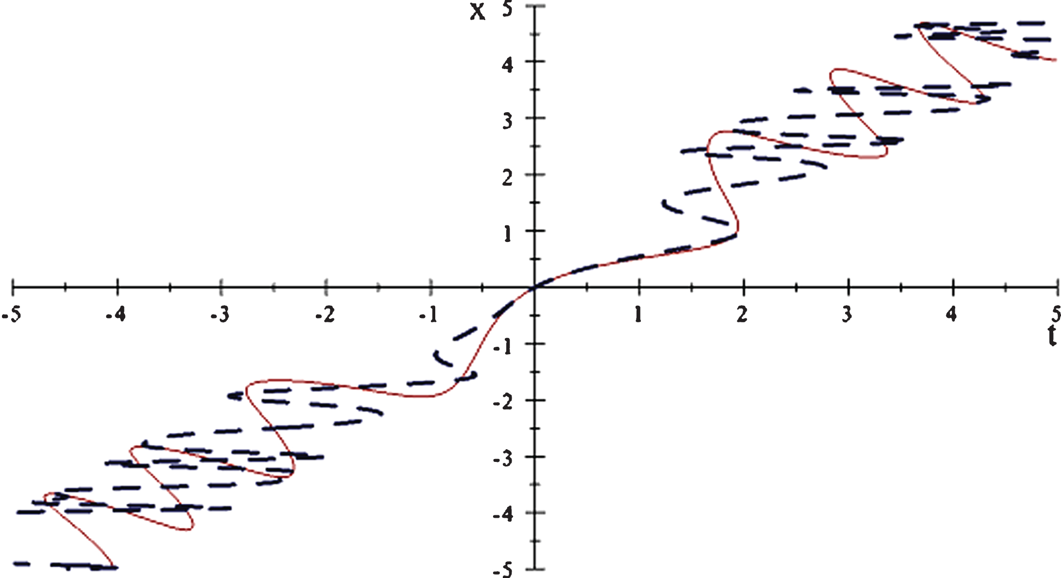
The Implicit function theorems contribute a key role in economics, particularly in the analysis of comparative statics and constrained optimization problems. Usually when we verbalize of functions, we are speaking about explicit functions of the form x = f (t). In mathematical problems many times we have to face an equation in x and t, for example, $t + \sin (xt) - x = 0,$ which may not be solvable for x. The solutions to this type of equations are a set of points {(x, t)} satisfying a relation of form f (x, t) = 0, which is called an implicit function. Implicit functions are often not actually functions in the strict definition of the text, because they often have multiple values x for a single value t. It can be seen in figure (3) on next page, which is the representation of t + sin(xt) - x = 0.

Fig.3

Graph of implicit function.

It is noticed that, many implicit functions are complicated or unworkable to convert to explicit functions and must be treated in the available implicit form. However there may be an opportunity to dig out explicit restrictions of such relation to resolve a number of bugs during normal calculations. For example, compare the graph of t + sin(xt) - x = 0, x (t) = t + sin(t² + t sin t²) in figure (4) on next page.

Fig.4

Comparison of implicit relation with its explicit restriction.

Here it can be seen that both curves are same in interval $[\frac{- 1}{3}, 2] .$

Our objective in this section is to seek certain circumstances and assumptions under which one can approximate explicit function from the given implicit form. In the following, we apply our theorem 4 to generate an implicit function theorem. A fascinating example is established to justify the result.

Theorem 15. Let $G, E : ℝ^{m} \times [a, b] ⟶ ℝ^{m}$ and $f : ℝ^{m} ⟶ ℝ^{m}$ be continuous mappings such that $\begin{matrix} G (x, t) = E (x, t) + f (x) . \end{matrix}$ Suppose that for each $x \in (C [a, b], ℝ^{m}),$ there exists $y \in (C [a, b], ℝ^{m}),$ such that (fy) (t) = G (x (t) , t) and ${fx : x \in (C [a, b], ℝ^{m})}$ is complete. If there exists φ ∈ Δ^∗ such that for all $x_{1}, x_{2} \in (C [a, b], ℝ)$ and t ∈ [a, b] , $\begin{matrix} M (G (x_{1} (t), t) - G (x_{2} (t), t)) \\ \leq φ M (f (x_{1} (t)) - f (x_{2} (t))) . \end{matrix}$

Then the equation E (x, t) = 0 defines a unique continuous function x in terms of t .

Proof. Let $X = Y = (C [a, b], ℝ)$ and η : X ⟶ L - {0_L} be an arbitrary mapping. Define $d : X \times X \to ℝ$ as

Assume, for x ∈ X $\begin{matrix} ω_{x} (t) = G (x (t), t), \forall t \in [a, b] . \end{matrix}$

Define L-fuzzy mapping $Φ : X ⟶ F_{L} (X)$ and singlevalued mapping F : X → X as follows $\begin{matrix} (Φ_{x}) (g) = {\begin{matrix} η (x) & if g (t) = ω_{x} (t) \forall t \in [a, b] \\ 0_{L} & otherwise . \end{matrix} \end{matrix}$ $\begin{matrix} (F_{x}) (t) = f (x (t)) . \end{matrix}$

Take α_x = η (x), then α_x ∈ L - {0_L} and $\begin{matrix} ⋃_{x \in X} [Φ x]_{α_{x}} & = ⋃_{x \in X} {g \in X (Φ x) (g) = η (x)} \\ = ⋃_{x \in X} {ω_{x}} . \end{matrix}$ ⇒ ⋃_x∈X [Φx] _{α
_x} ⊆ FX .

Moreover, we obtain $\begin{matrix} H ([Φ x]_{α_{x}}, [Φ y]_{α_{y}}) = max_{t \in [a, b]} M (ω_{x} (t) - ω_{y} (t)), \end{matrix}$ and $\begin{matrix} d (Fx, Fy) = max_{t \in [a, b]} M (f (x (t)) - f (y (t))) . \end{matrix}$

By assumptions, we have $\begin{matrix} M ((ω_{x} (t) - ω_{y} (t)) & = M (G (x (t), t) - G (y (t), t)) \\ \leq φ (M (f (x (t)) - f (y (t)))) . \end{matrix}$

Hence all the conditions of Theorem 4 are satisfied to find a continuous function $u : [a, b] ⟶ ℝ^{m}$ such that u ∈ C_(F,Φ) ⋂ C_(F,Ψ) ≠ ∅ . That is, f ∘ u = ω_u and u will be a solution of the equation E (u, t) =0 .

As a simple example consider an implicit form E (x, t) = 10x⁷ (t - 1) + t then by the assumptions G (x, t) = 10x⁷ (t - 1) + t + 90x⁷, and f (x (t)) = 90x⁷ in the Theorem 15 one can easily find the explicit representation as $x = \sqrt[7]{\frac{1}{10} \frac{t}{1 - t}} .$

Now in the support of above theorem we furnish the following interesting example to approximate explicit form of a nontrivial implicit function.

Example 16. Consider the implicit equation $(7) t + sin (x^{3} t) - x^{3} = 0$ (7) in space $X = C [\frac{- 1}{9}, \frac{1}{9}] .$ Let E (x, t) = t + sin(x³t) - x³ where $E : ℝ \times [\frac{- 1}{9}, \frac{1}{9}] \to ℝ$ and $f (x) = 4 x^{3} - \frac{5}{6} .$

Then, let $G (x, t) = t + sin (x^{3} t) + 3 x^{3} - \frac{5}{6} .$ $f (ℝ) = ℝ,$ hence $G (x, t) \in f (ℝ)$ for all x and t .

Consider, $\begin{matrix} x, t) - G (y, t) | & = & | t + sin (x^{3} t) + 3 x^{3} - \frac{5}{6} \\ - & t - sin (y^{3} t) - 3 y^{3} + \frac{5}{6} | \\ \leq & | sin (x^{3} t) - \\ sin & (y^{3} t) + 3 x^{3} - 3 y^{3} | \\ \leq & | sin (x^{3} t) - \\ sin & (y^{3} t) | + 3 | x^{3} - y^{3} | \\ \leq & | t | | x^{3} - y^{3} | + 3 | x^{3} - y^{3} | \\ \leq & \frac{11}{12} | 4 x^{3} - \frac{5}{6} - 4 y^{3} + \frac{5}{6} | \end{matrix}$

Hence both the conditions are verified.

Now we iterate the process to find an explicit form of the implicit equation given in (7) .

Here $\begin{matrix} G (x, t) = t + sin (x^{3} t) + 3 x^{3} - \frac{5}{6} \end{matrix}$

Consider an initial guess x₀ = 0 then $\begin{matrix} G (x_{0}, t) = t - \frac{5}{6} = f (x_{1}) = 4 x_{1}^{3} - \frac{5}{6} . \end{matrix}$

This implies that $x_{1} = \sqrt[3]{\frac{t}{4}} = u_{1} (t)$ ,

$x_{2} = \frac{1}{4^{1 / 3}} {(2 t + sin (\frac{t^{2}}{4}))}^{1 / 3} = u_{2} (t)$

and $\begin{matrix} x_{3} & = & \frac{1}{4^{1 / 3}} [t + sin (\frac{2 t^{2} + t sin (\frac{t^{2}}{4})}{4}) \\ + \frac{3}{4} (2 t + sin (\frac{t^{2}}{4}))]^{1 / 3} = u_{3} (t) . \end{matrix}$

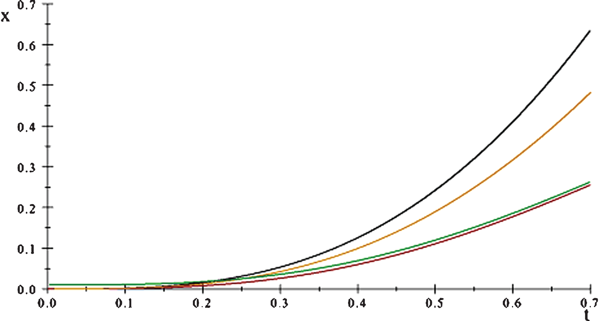
In Fig. 5 opening curve (from top) is the representation of explicit form x₂ = u₂ (t) obtained after 2nd iteration, 2nd curve is the graph of explicit form x₃ = u₃ (t) obtained after 3rd iteration, next curve represents 10th iteration and the original graph of implicit form (7) is shown by the last curve.

Fig.5

Graph of exact and approximate solutions.

Conclusion

Our work is committed to explore more relations among Hausdorff distance, fuzzy set theory and fixed point theory. We considered the central circumstances to demonstrate the presence of coincidence points of mappings that satisfies new common contraction conditions. The notion of Hausdorff distance is very useful in various zones of mathematics and computer science such as optimization theory, fractals and image computing. In real domain problems, game theory has applications in decision and policy making and administrative problems. It becomes difficult to assess the payoff of different stake holders due to the imprecise information and fuzzy situations. Fuzzy fixed point theorems can be applied to solve equilibrium problems in game theory if the payoff is signified by fuzzy sets and schemes are substituted by some fuzzy functions. In our daily life, catalogs are full of uncertainties, vagueness and imprecision. Traditional mathematical tools may not be beneficial to handle such difficulties. Some advanced representations such as fuzzy set theory, rough set theory and soft set theory are very useful in demonstrating and extracting the undetected realities in vague info group. Zhan et al. [34–37 , 40] and Zhang et al. [38, 39] played a vital role in soft and rough set theories. These models have been positively applied to intelligent systems, decision analysis, expert systems, machine learning, metro-logy, image processing, signal analysis, pattern recognition, game theory and many other fields. On the basis of the above research, we have proved a common coincidence point theorem for three mappings in which one is crisp mapping and other two mappings are L-fuzzy under a generalized φ-contraction condition on a metric space in association with the the Hausdorff distance. Then it is concluded that under the similar conditions there may be a coincidence point of a pair of multivalued mappings and a point to point mapping. A few corollaries are deduced to generalize many important results with the d_∞ metric on L-fuzzy sets. Moreover, it is shown that the integral equation $(h \circ ξ) (t) - λ \int_{a_{1}}^{a_{2}} Δ (t, s, ξ (s)) ds = j (t)$ can be solved in $(C [a, b], ℝ^{m})$ under the circumstances created in connection with hypothesis of a coincidence point theorem. Further, it is proved that under certain circumstances and assumptions one can approximate explicit function from the given implicit form. For authentication and embellishment of our result some stimulating and non-trivial examples are presented as well. Moreover, this work is based on lattice theory and L-fuzzy mappings in connection with level sets of L-fuzzy set to produce a chain of crisp configuration which is supple style to solve multi-functions domain problems.

Footnotes

Acknowledgements

The authors are highly grateful to the Associate Editor and the anonymous referees for their valuable comments and kind suggestions which helped to improve the quality of this paper.

References

Abu-Donia

H.M.

, Common fixed points theorems for fuzzy mappings in metric spaces under φ dollarcontraction condition, Chaos, Solitons and Fractals, 34, (2007), 538–543.

Azam

, Khan

MNA.

, Mehmood

, RadenoviÂt’c

and DoÅąenoviÂ’c

, Coincidence point of L-fuzzy sets endowed with graph, Revista de la Real Academia de Ciencias Exactas, FÃsicas y Naturales. Serie A. MatemÃąticas, (2017), 1–17.

Azam

, Mehmood

, Rashid

and Pavlovic

, L-fuzzy fixed points in cone metric spaces, J. Adv. Math. Stud, 9(1), (2016), 121–131.

Azam

, Fuzzy fixed points of fuzzy mappings via rational inequality, Hacettepe Journal of Mathematics and Statistics, 40(3), (2011), 421–431.

Azam

, Arshad

and Beg

, Common fixed point of fuzzy mappings under a contraction condition, Internat. Jour. Fuzzy Systems, 13(4), (2011), 383–389.

Azam

and Arshad

, A note on “Fixed point theorems for fuzzy mappings” by P. Vijayaraju and M. Marudai, Fuzzy Sets and Systems, 161, (2010), 1145–1149.

Azam

, Arshad

and Vetro

, On a pair of fuzzy φ- contractive mappings, Math. Comp. Modelling, 52, (2010), 207–214.

Azam

and Beg

, Common fixed points of fuzzy maps, Math. Comp. Modelling, 49, (2009), 1331–1336.

Azam

, Arshad

and Beg

, Fixed points of fuzzy contractive and fuzzy locally contractive maps, Chaos, Solitons & Fractals, 42(5), (2009), 2836–2841.

10.

Azam

, Waseem

and Rashid

, Fixed point theorems for fuzzy contractive mappings in quasi-pseudo-metric spaces, Fixed Point Theory and Applications, 2013(1), (2013), doi: 10.1186/1687-1812-2013-27.

11.

Azam

and Rashid

, A fuzzy coincidence theorem with applications in a function space, Journal of Intelligent and Fuzzy Systems, 27, (2014), 1775–1781.

12.

Das

P.C.

, On fuzzy normed linear space valued statistically convergent sequences, Proyecciones Journal of Mathematics, 36(3), (2017), 511–527.

13.

Heilpern

, Fuzzy mappings and fixed point theorems, J. Math. Anal. Appl, 83, (1981), 566–569.

14.

Goguen

J.A.

, L-fuzzy sets, J. Math. Anal. Appl, 18(1), (1967), 145–174.

15.

Hussain

, Khaleghizadeh

, Salimi

, Afrah

and Abdou

, A new approach to fixed point results in triangular intuitionistic fuzzy metric spaces, Abstract and Applied Analysis, 2014, (2014), 1–16.

16.

Kamran

, Common fixed points theorems for fuzzy mappings, Chaos Solitons and Fractals, 38, (2008), 1378–1382.

17.

Kutbi

M.A.

, Ahmad

, Azam

and Hussain

, On fuzzy fixed points for fuzzy maps with generalized weak property, Journal of Applied Mathematics, 2014.

18.

, Liu

and Zhan

, A survey of decision making methods based on certain hybrid soft set models, Artificial Intelligence Review, 47(4), (2017), 507–530.

19.

, Zhan

, Ali

MI.

and Mehmood

, A survey of decision making methods based on two classes of hybrid soft set models, Artificial Intelligence Review, 49(4), (2018), 511–529.

20.

Nadler

S.B.

, Multivalued contraction mappings, Pacific J. Math, 30, (1969), 475–488.

21.

El Naschi

M.S.

, On the uncertainty of Cantorian geometry and the two-slit experiment, Chaos, Soliton and Fractals, 9(3), (1998), 517–529.

22.

El Naschie

M.S.

, On the uniïňĄcation of heterotic strings theory, M theory and ∞^∞ theory, Chaos, Soliton and Fractals, 11(14), (2000), 2397–2407.

23.

Rashid

, Azam

and Mehmood

, L-fuzzy fixed points theorems for L-fuzzy mappings via β_{F
_L}-admissible pair, Sci. World J, 2014, (2014), 1–8.

24.

Rashid

, Kutbi

M.A.

and Azam

, Coincidence theorems via alpha-cuts of L-fuzzy sets with applications. Fixed Point Theory Appl, 2014(212), (2014), 1–16.

25.

Rashid

, Shahzad

and Azam

, Fixed point theorems for L-fuzzy mappings in quasi-pseudo metric spaces, Journal of Intelligent and Fuzzy Systems, 32(2017), 499–507.

26.

Shatanawi

, Some fixed point results for a generalized ψ-weak contraction mappings in orbitally metric spaces, Chaos, Solitons & Fractals, 45(4), (2012), 520–526.

27.

Shoaib

, Kumam

, Phiangsungnoen

and Mahmood

, Fixed point results for fuzzy mappings in a b-metric space, Fixed point theory and Applications, 1, (2018), 1–12.

28.

Tripathy

B.C.

and P.C.

Das

, On convergence of series of fuzzy real numbers, Kuwait journal of science and engineering, 39(1A), (2012), 57–70.

29.

Tripathy

B.C.

, Paul

and Das

N. R.

, Banach’s and Kannan’s fixed point results in fuzzy 2-metric spaces, Proyecciones. Journal of Mathematics, 32(4), (2013), 359–375.

30.

Tripathy

B.C.

, Paul

and Das

N. R.

, Fixed point and periodic point theorems in fuzzy metric space, Songklanakarin J. Sci. Technol, 37(1), (2015), 89–92.

31.

Tripathy

B.C.

and Paul

and Das

N. R.

, A fixed point theorem in a generalized fuzzy metric space, Boletim da Sociaedade Paranaense de Mathematica, 32(2), (2014), 221–227.

32.

Wang

, Zhan

, Ali

MI.

and Mehmood

, A study on z-soft rough fuzzy semigroups and its decision-making, International Journal for Uncertainty Quantification, 8(1), (2018), 1–22.

33.

Zadeh

L.A.

, Fuzzy sets, Inf. Control, 8(3), (1965), 338–353.

34.

Zhan

, Ali

MI.

and Mehmood

, On a novel uncertain soft set model: Z-soft fuzzy rough set model and corresponding decision making methods, Applied Soft Computing, 56, (2017), 446–457.

35.

Zhan

and Zhu

, A novel soft rough fuzzy set: Z-soft rough fuzzy ideals of hemrings and corresponding decision making, Soft Computing, 21(8), (2017), 1923–1936.

36.

Zhan

, Sun

and Alcantud

J.C.R.

, Coverings based multigranulation (I,T)-fuzzy rough set models and applications in multi-attribute group decision making, Information Science, 476, (2019), 290–318.

37.

Zhan

and Xu

, Two types of coverings based multigranulation rough fuzzy sets and applications to decision making, Artif Intell., Rev (2018) https://doi.org/10.1007/s10462-018-9649-8.

38.

Zhang

, Zhan

and Alcantud

J.C.R.

, Novel classes of fuzzy soft β-coverings-based fuzzy rough sets with applications to multi-criteria fuzzy group decision making, Soft Comput, (2018), https://doi.org/10.1007/s00500-018-3470-9.

39.

Zhang

and Zhan

, Fuzzy soft β-covering based fuzzy rough sets and corresponding decision-making applications, Int. J. Mach. Learn. Cybern, (2018), doi: 10.1007/s13042-018-0828-3.

40.

Zhan

and Wang

, Certain types of soft coverings based rough sets with applications, Int. J. Mach. Learn. Cyber. doi: 10.1007/s13042-018-0785-x, (2018).

41.

Zhou

, Wu

W. Z.

and Zhang

W. X.

, Properties of the cutsets of intuitionistic fuzzy relations, Fuzzy Systems and Mathematics, 23(2), (2009), 110–115.