Roughness in Substructures of Skew Lattices

1 Introduction

Rough set theory, proposed by Pawlak [20], is a mathematical tool for dealing with uncertainty and vagueness that has been widely applied to various fields such as pattern recognition, data mining and automated knowledge acquisition (see [14–18, 22]). Using the equivalence classes of an equivalence relation on a universe, Pawlak constructed a lower and an upper approximation for every subset of that universe. Rough set theory can be viewed as the extension of ZF set theory described by Mani [19].

Skew lattices were introduced by J. Leech [13] in 1989, which are one of the most successful non-commutative generalizations of lattices. Many researchers have contributed to skew lattice theory in recent years. In general, a skew lattice S is an algebra (S, ∨ , ∧), where S is a non-empty set, and both ∨ and ∧ are binary operations on S satisfying associative, idempotent and two special absorption laws. If S is also commutative, then it is a lattice. Although, a skew lattice has a natural quasi-order “⪯” (y ⪯ x ⇔ x ∨ y ∨ x = x or y ∧ y ∧ y = y) and a natural partial order “≤” (y ≤ x ⇔ x ∨ y = y ∨ x = x or x ∧ y = y ∧ x = y), it is generally not an ordered structure in which its binary operations ∨ and ∧ cannot be determined by either order relation. From the perspective of semigroup theory, both the algebraic reducts (S, ∨) and (S, ∧) of a skew lattice S are bands, that is, semigroups in which every element is idempotent. Hence, a number of basic concepts and results from semigroup theory have been passed on to skew lattice theory. For example, in the skew lattice, the equivalence relations L , R and D are generalizations of Green’s Relations arising in semigroup theory, which are of critical importance in investigating different subvarieties of skew lattices. In particular, they have been useful in analyzing properties (and their corresponding subvarieties) such as distributivity, cancelation, normally and symmetry. On the other hand, as some of these topics indicate, there has also been a focus on extending concepts and results about lattices to skew lattices. It is worth noting that the papers [1, 11] provide non-commutative versions of Stone duality for Boolean lattices and Priestly duality for bounded distributive lattices with the help of sheaf theory and category theory. Skew lattices have demonstrated in their relevance in Econometrics, Computer Science, Logic and elsewhere [3–5, 23].

The main purpose of this paper is to discuss the rough substructures of skew lattices. Actually, rough substructures of algebraic systems were the interesting topics for many scholars. For example: Jun investigated the properties of lower and upper approximation in gamma semigroups in [10]. Biswas and Nanda [6] proposed the notion of rough subgroups and discussed their basic properties. Zhan and Davvaz studied the notions of rough soft sets and rough soft rings [9, 28]. Kuroki [12] and Xiao [24] respectively introduced the notions of rough ideals and rough prime ideals in a semigroup; Xiao and Li [25, 26] considered rough ideals of a lattice and rough subsets induced by ideals. In this paper, six substructures of a skew lattice are studied in connection with rough approximations: sub-skew lattices and sublattices, ideals and filters, as well as s-ideals and s-filters.

The paper is organized as follows: In Section 2, we introduce some basic concepts and results on rough sets and skew lattices. In Section 3, we discuss the properties of rough subsets of skew lattices relative to a given congruence relation θ. Section 4 proposes upper (lower) rough sub-skew lattices, upper (lower) rough ideals and their duals, upper (lower) rough filters, upper (lower) rough s-ideals and s-filters, and upper (lower) rough sublattices. We study their properties relative to an arbitrary congruence and to the three special congruence relations L , R and D in particular. In Section 5, we extend some of these properties to products and quotients of skew lattices. In Section 6, homomorphic images of rough substructures are considered. We give a conclusion inSection 7.

2 Some preliminaries on rough sets and skew lattices

In this section, we will recall some elementary concepts about skew lattices and rough sets, and some important results which will be widely used in the following sections.

A skew lattice is an algebra (S, ∨ , ∧), where S is a non-empty set, both ∨ and ∧ are binary operations on S, called the meet and join, respectively, which are closed in S, and satisfy the following identities:

: (x ∨ y) ∨ z = x ∨ (y ∨ z) and (x ∧ y) ∧ z = x ∧ (y ∧ z);

The identities introduced above in SL₁ ∼ SL₃ are known as the associative laws, the idempotent laws and the absorption laws. Especially, the condition SL₃ and the condition SL 3 ′ are equivalent in skew lattices. Clearly, a lattice is in fact a skew lattice satisfying the commutaive laws:

: x ∨ y = y ∨ x and x ∧ y = y ∧ x.

Definition 2.1. Let (S, ∨ , ∧) be a skew lattice. A relation θ on the S is called left compatible, if ( s , t ) ∈ θ ⇒ ( a ∨ s , a ∨ t ) ∈ θ and ( a ∧ s , a ∧ t ) ∈ θ , ∀ s , t , a ∈ S ; and right compatible, if ( s , t ) ∈ θ ⇒ ( s ∨ a , t ∨ a ) ∈ θ and ( s ∧ a , t ∧ a ) ∈ θ , ∀ s , t , a ∈ S . It is called compatible, if

  ∀ s, t, s′, t′ ∈ S, (s, s′) ∈ θ,(t, t′) ∈ θ ⇒ 

  (s ∨ t, s′ ∨ t′) ∈ θ, (s ∧ t, s′ ∧ t′) ∈ θ .

A left [right] compatible equivalence relation is called a left [right] congruence relation. A compatible equivalence relation is called a congruence relation.

From Definition 2, we know that a relation θ on a skew lattice S is a congruence relation if and only if it is both a left and a right congruence relation.

Like a lattice, a skew lattice has a natural partial order “≤” defined between elements as follows: y ≤ x ⇔ x ∨ y = y ∨ x = x ⇔ x ∧ y = y ∧ x = y ; and a natural quasi-order “⪯” defined as follows: y ⪯ x ⇔ x ∨ y ∨ x = x ⇔ y ∧ x ∧ y = y . The algebraic reducts of a skew lattice (S, ∨) and (S, ∧) are regular bands, which satisfy the identities: x ∨ y ∨ z = x ∨ z , if y ⪯ x , z and x ∧ y ∧ z = x ∧ z , if x , z ⪯ y . By using the quasi-order, an equivalence relation can be induced, denoted by D , which is an important equivalence relation in skew lattice theory together with the equivalence relations L and R . The three equivalence relations above are respectively defined as follows:

x D y ⇔ y ⪯ x and x ⪯ y ⇔ x ∨ y ∨ x = x and y ∨ x ∨ y = y ⇔ y ∧ x ∧ y = y and x ∧ y ∧ x = x;

The three equivalence relations presented above are skew lattice congruences that were derived from the Green’s Relations in semigroup theory. The relations L and R refine D , with L ∘ R = R ∘ L = D , L ∩ R = Δ , where Δ denotes the identity relation. Among the three congruence relations, the blocks of the quotient algebra S / D are rectangular skew lattices, in which for any two elements x, y in the same block, x ∨ y ∨ x = x and y ∨ x ∨ y = y, and likewise y ∧ x ∧ y = y and x ∧ y ∧ x = x.

The following Decomposition Theorems for skew lattices are the frameworks of fundamental theory of skew lattices.

Theorem 2.2. [First Decomposition Theorem](J. Leech, 1989) Let (S, ∨ , ∧) be a skew lattice. Then the equivalence relation D as defined above forms a congruence relation. The equivalence classes are the maximal rectangular subalgebras of S, while the quotient algebra S / D is the maximal lattice image of S.

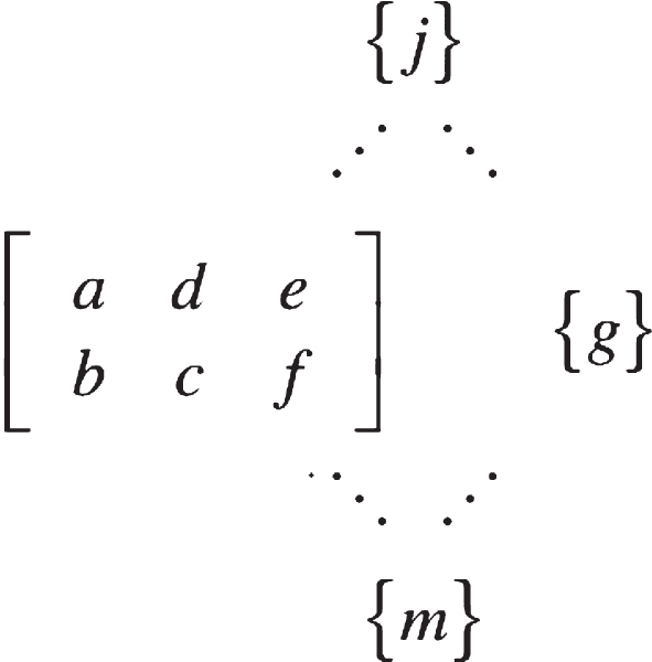
From the above theorem, we know that every skew lattice is a lattice of sub-rectangular skew lattices of itself. For some insight, we consider a skew diamond consisting of a pair of incomparable D -classes, A and B, their join class J and their meet class M in the lattice of D -classes S / D .

Theorem 2.3. [13] Let (S, ∨ , ∧) be a skew lattice and A and B equivalence classes in S. Suppose that A ≤ B in S / D , then for each a in A, there exists b in B such that a ≤ b, and dually, for each b in B, there exists a in A such that a ≤ b. In general, let J and M be equivalence classes such that J = A ∨ B, and M = A ∧ B in S / D . Let j ∈ J be given and pick a ∈ A and b ∈ B such that a, b ≤ j in S. Then j = a ∨ b = b ∨ a in S. Thus, in S, J = {a ∨ b ∣ a ∈ A, b ∈ B, and a ∨ b = b ∨ a}. Similar remarks hold for M and ∧.

Remark 2.4. Clearly, in Theorem 2 the equivalence class J contains all individual joins a ∨ b and b ∨ a for an a in the class A and an b in the class B, with a ∨ b = b ∨ a in some cases. It turns out that every member of J can be expressed as some commuting join. Similar remarks hold for M and ∧.

In universal algebras, skew lattices form a variety of algebras. Two particular subvarieties arise in a fundamental decomposition of skew lattices. Right handed skew lattices are the skew lattices that satisfy the identities: x ∧ y ∧ x = y ∧ x and x ∨ y ∨ x = x ∨ y . Dually, the left handed skew lattices are the skew lattices satisfy the identities: x ∧ y ∧ x = x ∧ y and x ∨ y ∨ x = y ∨ x . The following theorem, called the Second Decomposition Theorem for skew lattices, describes another decomposition that is related to the congruences L and R .

Theorem 2.5. [13] [Second Decomposition Theorem](J. Leech, 1989) Let (S, ∨ , ∧) be a skew lattice. Then S is biregular. Thus L is a congruence relation on S and S L = S / R is the maximal left handed image of S, with the induced homomorphism S ⟶ S / R being bijective between corresponding L -classes. Dually, R is also a congruence relation and S R = S / L forms the maximal right handed image of S, with the induced homomorphism S ⟶ S / L being bijective between corresponding R-classes. To within isomorphism, every skew lattice uniquely decomposes as the fibred product of a right handed skew lattice with a left handed skew lattice over a common underlying maximal image S / D .

In what follows, we recall the definitions of some substructures of a skew lattice.

Definition 2.6. [13] Let S be a skew lattice and ∅ ≠ I ⊆ S. Then I is a sub-skew lattice if it is closed under ∨, ∧.

Definition 2.7. [13] Let S be a skew lattice and ∅ ≠ A ⊆ L. Then A is a sublattice if a, b ∈ A imply b ∨ a = a ∨ b ∈ A, a ∧ b = b ∧ a ∈ A.

Definition 2.8. An s-ideal I of S is a sub-skew lattice of S such that for all a ∈ S and b ∈ I, a ⪯ b implies a ∈ I; Duality, an s-filter F of S is also a sub-skew lattice of S such that for all b ∈ S and a ∈ I, a ⪯ b implies b ∈ I.

Definition 2.9. [13] An ideal I of S is a sublattice of S such that for all a ∈ S and b ∈ I, a ≤ b implies a ∈ I. Dually, a filter F of S is also a sublattice of S such that for all b ∈ S and b ∈ I, a ≤ b impliesb ∈ I.

We denote the collection of all s-ideals in a skew lattice S by 𝕊𝕀 ( S ) and the collection of all ideals of S by 𝕀 ( S ) . Dually, we denote the collection of all s-filters in a skew lattice S by 𝕊𝔽 ( S ) and the collection of all filters of S by 𝔽 ( S ) .

Next, we will recall some basic concepts in rough set theory.

Definition 2.10. A skew lattice S is normal if it satisfies the identity x ∧ y ∧ z ∧ w = x ∧ z ∧ y ∧ w; equivalently, S is normal if for any x ∈ S, its down set, ↓ x = {u ∈ S ∣ u ≤ x} is a sublattice, and in particular is commutative. More generally, if A is sublattice of a normal skew lattice S, then ↓A = {u ∈ S ∣ ∃ x ∈ A suchthat  u ≤ x} is also a sublattice of S.

In the dual fashion, a conormal skew lattice is defined in terms of ∨. Here, if A is a sublattice of S, then ↑A = {u ∈ S ∣ ∃ x ∈ A suchthat  x ≤ u} is also a sublattice of S.

Example 2.11. (1) The center Z _S of a skew lattice is the set of all elements that both ∨-commutative and ∧-commutative with each element of S. Z _S turns out to be the union of all singleton D -classes in S (and thus could be empty!). If S is normal, then Z _S is in fact an s-ideal of S (and thus an ideal). But if S is conormal, then Z _S is an s-filter of S (and thus a filter). (2) A lattice section of a skew lattice S is a sublattice S₀ that intersects uniquely with each D -class of S. A lattice section of S, if it exists, is an internal copy of the maximal lattice image S / D of S.

Definition 2.12. An approximation space is a pair (X, θ), where X is a non-empty set and θ is an equivalence relation on X. Let A be a non-empty subset of X, θ_- (A) = {x ∈ X ∣ [x]  _θ  ⊆ A} and θ^- (A) = {x ∈ X ∣ [x]  _θ  ∩ A ≠ ∅}, then θ_- (A) and θ^- (A) are called, respectively, the θ-lower and θ-upper approximations of A. (θ_- (A) , θ^- (A)) is called a rough set with respect to θ, if θ_- (A) ≠ θ^- (A). If a subset A ⊆ X satisfies θ_- (A) = θ^- (A), then A is called a definable set of (X, θ). We denote all the definable sets of (X, θ) by 𝔻 θ ( X ) . It’s clear that ∅ , X ∈ 𝔻 θ ( X ) and 𝔻 θ ( X ) forms a Boolean algebra under ∩, ∪, \, ∅.

Furthermore, it would be worth to mentioning that a subset A is definable set of (X, θ) precisely, when it is a union of θ-equivalence classes. Thus, θ_- (A) is the unique maximal θ-definable subset of A while θ^- (A) is the unique minimal θ-definable subset containing A.

Example 2.13. For the Green’s equivalence relations D ,  R and L : The center Z _S is definable relative to D , being the union of all singleton D -classes. If S has a lattice section S₀, then D - ( S 0 ) = Z S and D - ( S 0 ) = S . Also, L - ( S 0 ) = { x ∈ S 0 ∣ D x = R x } and L - ( S 0 ) = ⋃ { L x ∣ x ∈ S 0 } . Similarly, R - ( S 0 ) = { x ∈ S 0 ∣ D x = L x } and R - ( S 0 ) = ⋃ { R x ∣ x ∈ S 0 } . Here, D x , L x and R x denote respectively D , L and R congruence classes of x.

Theorem 2.14. Let θ and η be equivalence relations on a non-empty set X. If A and B are non-empty subsets of X, then:

θ_- (A) ⊆ A ⊆ θ^- (A); if either ⊆ is =, then so is the other and A is definable;

3 Rough subsets in skew lattices

In what follows, let A be a non-empty subset of the skew lattice S. Then (θ_- (A) , θ^- (A)) is a rough subset of S with respect to an equivalence relation θ, where θ_- (A) ≠ θ^- (A). In this section, we denote the join and meet of two subsets A and B in a skew latticeby A ∨ B = { x ∨ y ∣ x ∈ A , y ∈ B } , A ∧ B = { x ∧ y ∣ x ∈ A , y ∈ B } ; and for families of subsets of the skew lattice S, {A _i  ∣ i ∈ I}, {B _j  ∣ j ∈ J}, ( ⋃ i ∈ I A i ) ∨ ( ⋃ j ∈ J B j ) = ⋃ i ∈ I ; j ∈ J ( A i ∨ B j ) ; ( ⋃ i ∈ I A i ) ∧ ( ⋃ j ∈ J B j ) = ⋃ i ∈ I ; j ∈ J ( A i ∧ B j ) . We say that a congruence relation θ on a skew lattice S is join-complete, if [ a ] θ ∨ [ b ] θ = [ a ∨ b ] θ , ∀ a , b ∈ S . Dually, θ is said to be meet-complete, if [ a ] θ ∧ [ b ] θ = [ a ∧ b ] θ , ∀ a , b ∈ S . A congruence relation θ is said to be complete, if it is both join-complete and meet-complete. It is obvious that the congruence relation D is complete based on Theorem 2 and Theorem 2. Some important instances of complete congruences are:

Theorem 3.1. D , R , L are complete congruences on any skew lattice S.

Proof. That D is complete is clear from Theorem 2.

We show that L is meet complete. That it is join complete and that R is both meet and join complete are shown similarly. So, let π : S ⟶ S / R be the canonical epimorphism. D = L on S / R and π is bijective between corresponding L -classes.

Given a, b ∈ S, L a ∧ L b is at least contained in L a ∧ b . Thus, π ( L a ∧ L b ) is at least contained in π ( L a ∧ b ) . Moreover, conditional equality holds in which π ( L a ∧ L b ) = π ( L a ∧ b ) if and only if L a ∧ L b = L a ∧ b . But from π ( L a ∧ L b ) = π ( L a ) ∧ π ( L b ) = L π ( a ) ∧ L π ( b ) = D π ( a ) ∧ D π ( b ) = D π ( a ) ∧ π ( b ) = D π ( a ∧ b ) = L π ( a ∧ b ) = π ( L a ∧ b ) and the bijectivity of π on L -classes, L a ∧ L b = L a ∧ b follows. Thus, L is meet complete and similarly it is join complete, and likewise for R . ■

We know that lattices can be viewed as a special case of skew lattices. Hence, many properties of rough sets in lattices can be generalized to skew lattices. We will show several results of the generalizations in the following.

Proposition 3.2. Let θ be a congruence relation on a skew lattice S, A and B non-empty subsets of S. Then

θ^- (A) ∨ θ^- (B) ⊆ θ^- (A ∨ B);

Proof. We only prove (1) and (3). (2) and (4) can be proved similarly.

(1) θ^- (A) ∨ θ^- (B) = (⋃ _a∈A [a]  _θ ) ∨ (⋃ _b∈B [b]  _θ ) = ⋃ _a∈A;b∈B ([a]  _θ  ∨ [b]  _θ ) ⊆ ⋃ _a∈A;b∈B [a ∨ b]  _θ  = θ^- (A ∨ B).

(3) The first assertion follows upon replacing the ⊆ with =. The second assertion follows from observing that [a]  _θ  ⊆ A and [b]  _θ  ⊆ B imply [a ∨ b]  _θ  = [a]  _θ  ∨ [b]  _θ  ⊆ A ∨ B. ■

Corollary 3.3. For any skew lattice S and subsets A and B:

D - ( A ) ∨ D - ( B ) = D - ( A ∨ B ) and D - ( A ) ∧ D - ( B ) = D - ( A ∧ B ) ;

Proposition 3.4. Let θ₁, θ₂ be congruence relations on a skew lattice S and A a non-empty subset of S. Then

( θ 1 ∩ θ 2 ) - ( A ) ⊆ θ 1 - ( A ) ∩ θ 2 - ( A ) ;

Proof. (1), (2) are obvious by Theorem 2 (7). ■

Remark 3.5. In any variety of algebras it is well-known that if θ ∘ η = η ∘ θ, then η ∨ θ  = η ∘ θ. This holds in particular for skew lattices.

Theorem 3.6. Let θ, η be congruence relations on a skew lattice S such that θ ∘ η = η ∘ θ. If A is a sub-skew lattice of S, then

θ^- (A) ∨ η^- (A) ⊆ (η ∨ θ) ^- (A); η^- (A) ∨ θ^- (A) ⊆ (η ∨ θ) ^- (A);

Proof. (1) If c ∈ θ^- (A) ∨ η^- (A), then c = a ∨ b with a ∈ θ^- (A), b ∈ η^- (A). Thus, there exist x, y ∈ A such that x ∈ [a]  _θ  ∩ A, y ∈ [b]  _η  ∩ A. Since A is a non-empty sub-skew lattice of S, we have x ∨ y ∈ A. Thus, x ∨ y ≡ a ∨ y (mod θ); a ∨ y ≡ a ∨ b (mod η) which imply x ∨ y ≡ a ∨ b (mod η ∘ θ). Hence, a ∨ b ∈ (η ∨ θ) ^- (A). The proof of the second inclusion is similar.

OPEN IN VIEWER

Fig.1

The skew lattice S₉.

(2) The proof is similar to (1). ■

In particular, corresponding statements hold for sublattices, ideals, filters, etc.

The example below shows that the converse of Theorem 3 do not hold in general.

Example 3.7. Let S₉ be the skew lattice with operations defined on S = {a, b, c, d, e, f, g, m, j} by the Cayley tables below. R , Δ be congruence relations on S₉. A={a}, Δ ∘ R = R ∘ Δ = R , Δ ∘ L = L ∘ Δ = L , S / R = { { j } , { a , b } , { c , d } , { e , f } , { g } , { m } } ; S / L = { { j } , { a , d , e } , { b , c , f } , { g } , { m } } ; S / D ={{j} , {a, b, c, d, e, f} , {g} , {m}}; S/Δ = {{j} , {a} , {d} , {e} , {b} , {c} , {f} , {g} , {m}}; Δ^- (A) = {a}; R - ( A ) ={a, b}; D - ( A ) = { a , b , c , d , e , f } . But, R - ( A ) ∨ Δ - ( A ) ≠ Δ - ( A ) ∨ R - ( A ) = { a } ⊆ R - ( A ) ; Δ - ( A ) ∧ R - ( A ) ≠ R - ( A ) ∧ Δ - ( A ) = { a } ⊆ R - ( A ) . We also can get the similar results with Δ ∘ L = L ∘ Δ . So, the inverse inclusions about sublattice which is similar as Theorem 3 also do not hold in general, too.

Theorem 3.8. Let θ, η be congruence relations on a skew lattice S and A is a non-empty subset of S.

If θ ∘ η = η ∘ θ, then θ_- (η_- (A)) = η_- (θ_- (A)).

Proof. (1) The proof is similar as that of statement (2), we show that in the following.

(2) Suppose x ∈ θ^- (η^-) (A), there exists y ∈ η^- (A) such that x ≡ y (mod θ). It follows that there exists z ∈ A such that y ≡ z (mod η). Thus, x ≡ z (mod θ ∘ η). Since θ ∘ η = η ∘ θ, there exists y₀ ∈ S such that x ≡ y₀ (mod η) and y₀ ≡ z (mod θ). So, y₀ ∈ θ^- (A). Thus, x ∈ η^- (θ^-) (A). Therefore, θ^- (η^- (A)) ⊆ η^- (θ^-) (A). Similarly, it can be proved that η^- (θ^-) (A) ⊆ θ^- (η^- (A))

Conversely, Let (a, b) ∈ θ ∘ η, we have a ∈ θ^- (η^- ({b})) = η^- (θ^-) ({b}). Then, there exists y ∈ θ^- ({b}) such that (a, y) ∈ η. So, (y, b) ∈ θ. Thus, we obtain (a, b) ∈ η ∘ θ. ■

Short examples about commuting congruences on skew lattices can be easily found in the following: For any skew lattice S, D , R , L , θ are congruences on S, it follows that R ∘ L = L ∘ R = L ∨ R and θ ∘ D = D ∘ θ = D ∨ θ .

Let θ be a congruence relation and A a non-empty subset of S. A is said to be an upper rough s-ideal [ideal, sublattice, sub-skew lattice] of S, if θ^- (A) is an s-ideal [ideal, sublattice, sub-skew lattice]. A is said to be a lower rough s-ideal [ideal, sublattice, sub-skew lattice] of S, if θ_- (A) is an s-ideal [ideal, sublattice, sub-skew lattice]. A is said to be a rough s-ideal [ideal, sublattice, sub-skew lattice] of S, if both θ^- (A) and θ^- (A) are s-ideals [ideals, sublattices, sub-skew lattices]. We denote the set of all upper [lower] rough s-ideals with respect to a congruence relation θ of S by 𝕊𝕀 ( θ - ( S ) ) [ 𝕊𝕀 ( θ - ( S ) ) ] .

Theorem 4.1. Let S be a skew lattice with a bottom element 0 (with respect to the preorder “⪯”), then 𝕊𝕀 ( S ) is a topped ∩-structure.

Proof. It is easily to show that S is an s-ideal, i.e., S ∈ 𝕊𝕀 ( S ) . Let { A i ∣ i ∈ I } ⊆ 𝕊𝕀 ( S ) , then 0∈ ⋂ _i∈IA _i  ≠ ∅. Thus, it is easy to know that ⋂_i∈IA _i is an s-ideal. ■

Theorem 4.2. Let S be a skew lattice with a bottom element and θ is a congruence relation on S. Then 𝕊𝕀 ( θ - ( S ) ) is a topped ∩-structure.

Proof. Let { S i ∣ i ∈ I } ⊆ 𝕊𝕀 ( θ - ( S ) ) , then θ_- (S _i ) is an s-ideal of S for any i ∈ I. Since θ_- (⋂ _i∈IS _i ) = ⋂ _i∈Iθ_- (S _i ), θ_- (⋂ _i∈IS _i ) is also an s-ideal of S. Thus ⋂ i ∈ I S i ∈ 𝕊𝕀 ( θ - ( S ) ) . It is clear that S ∈ 𝕊𝕀 ( θ - ( S ) ) . So, 𝕊𝕀 ( θ - ( S ) ) is a topped ∩-structure. ■

Theorem 4.3. Let θ be a congruence relation on a skew lattice S. Then relative to θ: If A is a sub-skew lattice of S, then A is an upper rough sub-skew lattice, In particular:

If A is a sublattice of S, then A is an upper rough sub-skew lattice;

Proof. Let π : S → S/θ be the canonical homomorphism onto S/θ. The theorem’s main statement and (1) follow from the following basic facts about sub-skew lattices. (2) and (3) follow from similar basic facts about s-ideals and s-filters:

If A is a sub-skew lattice (s-ideal) of S, then π [A] is a sub-skew lattice (s-ideal) of π [S];

Since sub-skew lattices and sublattices are upper rough sub-skew lattices relative to θ, and s-ideals (s-filters) are upper rough s-ideals (s-filters) relative to θ, respectively. A nature question is whether the ideals (filters) are upper rough s-ideals (s-filters) relative to θ. In general the answer is no.

Example 4.4. Consider the rectangular skew lattice on {a, b} and determined by a ∧ b = b = b ∨ a. Trivially {a} forms an ideal (filter). But L - { a } = a is not an s-ideal (s-filter).

However:

Corollary 4.5. If A is an ideal of S, then A is an upper rough s-ideal relative to the congruence D .

Proof. It is easy to know that ⋃ { D a ∣ a ∈ A } is an s-ideal, hence the corollary above is straightforward. ■

Theorem 4 shows that the upper approximation of a sub-skew lattice [s-ideal] is a sub-skew lattice [s-ideal], but the case of the lower approximation does not hold in general because if [a]  _θ  ⊆ A, [b]  _θ  ⊆ A, then [a]  _θ  ∨ [b]  _θ  ⊆ A. However, [a]  _θ  ∨ [b]  _θ  ⊆ [a ∨ b]  _θ only imply that [a∨ b]  _θ  ∩ A ≠ ∅. We can not get [a ∨ b]  _θ  ⊆ A in general.

Theorem 4.6. Let θ be a complete congruence relation on a skew lattice S and A be a non-empty subset of S.

If A is a sub-skew lattice of S, then θ_- (A) is, if it is nonempty, a sub-skew lattice of S;

Proof.

(1) Suppose a, b ∈ θ_- (A), then [a]  _θ  ⊆ A and [b]  _θ  ⊆ A. Now that θ is both join-complete andmeet-complete, we have {x ∨ y ∣ x ∈ [a]  _θ , y ∈ [b]  _θ } = [a]  _θ  ∨ [b]  _θ  = [a ∨ b]  _θ and {x ∧ y ∣ x ∈ [a]  _θ , y ∈ [a]  _θ } = [a]  _θ  ∧ [b]  _θ  = [a ∧ b]  _θ . Since A is a sub-skew lattice, we have {x ∨ y ∣ x ∈ [a]  _θ , y ∈ [a]  _θ } ⊆ A and {y ∨ x ∣ x ∈ [a]  _θ , y ∈ [a]  _θ } ⊆ A; {x ∧ y ∣ x ∈ [a]  _θ , y ∈ [a]  _θ } ⊆ A and {y ∧ x ∣ x ∈ [a]  _θ , y ∈ [a]  _θ } ⊆ A. So, [a ∨ b]  _θ , [b ∨ a]  _θ , [a ∧ b]  _θ , and [b ∧ a]  _θ  ⊆ A. It follows that b ∨ a, a ∨ b, b ∧ a, a ∧ b ∈ θ_- (A). Therefore, θ_- (A) is a sub-skew lattice.

(2) If a, b ∈ θ_- (A), then [a]  _θ  ⊆ A and [b]  _θ  ⊆ A.Now that A is a sublattice, we have x ∨ y = y ∨ x and x ∧ y = y ∧ x for any x ∈ [a]  _θ , y ∈ [b]  _θ . Since θ is both join-complete and meet-complete, we have [a ∨ b]  _θ  = [a]  _θ  ∨ [b]  _θ  = {x ∨ y ∣ x ∈ [a]  _θ , y ∈ [b]  _θ } = {y ∨ x ∣ x ∈ [a]  _θ , y ∈ [b]  _θ } = [b ∨ a]  _θ  ⊆ A ; [a ∧ b]  _θ  = [a]  _θ  ∧ [b]  _θ  = {x ∧ y ∣ x ∈ [a]  _θ , y ∈ [b]  _θ } = {y ∧ x ∣ x ∈ [a]  _θ , y ∈ [b]  _θ } = [b ∧ a]  _θ  ⊆ A. Therefore, b ∨ a = a ∨ b, b ∧ a = a ∧ b ∈ θ_- (A). Thus, it follows that θ_- (A) is a sublattice.

(3) Since A is an s-ideal, then A is an sub-skew lattice. According to (1), a ∨ b, b ∨ a ∈ θ_- (A) hold, for all a, b ∈ θ_- (A). Let x ∈ S, y ∈ θ_- (A) and x ⪯ y, then [x]  _θ  ⊆ S, [y]  _θ  ⊆ A. Since θ is meet-complete, we have [x ∧ y ∧ x]  _θ  = [x]  _θ  ∧ [y]  _θ  ∧ [x]  _θ  = {a ∧ b ∧ c ∣ a, c ∈ [x]  _θ , b ∈ [y]  _θ }. It is easy to see that a ∧ b ∧ c ⪯ b for all a ∧ b ∧ c ∈ {a ∧ b ∧ c ∣ a, c ∈ [x]  _θ , b ∈ [y]  _θ }. Hence, [x ∧ y ∧ x]  _θ  = {a ∧ b ∧ c ∣ a, c ∈ [x]  _θ , b ∈ [y]  _θ } ⊆ A by the definition of s-ideal. Since x ⪯ y, then [x]  _θ  ⊆ A, which implies x ∈ θ_- (A). Thus, θ_- (A) is an s-ideal.

(4) Let A be an ideal, then A is a sublattice in skew lattices. By (2), we have a ∨ b = b ∨ a ∈ θ_- (A) for all a, b ∈ θ_- (A). Let x ∈ S, y ∈ θ_- (A) and x ≤ y, then [x]  _θ  ⊆ S, [y]  _θ  ⊆ A. Since θ is meet-complete, we have [y ∧ x ∧ y]  _θ  = [y]  _θ  ∧ [x]  _θ  ∧ [y]  _θ  = {b ∧ a ∧ c ∣ b, c ∈ [y]  _θ , a ∈ [x]  _θ }. So, b ∨ c = c ∨ b ∈ A for all b, c ∈ [y]  _θ  ⊆ A because that A is an ideal of S. Thus, for all b ∧ a ∧ c ∈ {b ∧ a ∧ c ∣ b, c ∈ [y]  _θ , a ∈ [x]  _θ }, b ∧ a ∧ c ≤ b ∨ c implies b ∧ a ∧ c ∈ A. Therefore, [x]  _θ  = [y ∧ x ∧ y]  _θ  = {b ∧ a ∧ c ∣ b, c ∈ [y]  _θ , a ∈ [x]  _θ } ⊆ A. Thus, θ_- (A) is an ideal.

The proofs of (5), (6) are similar to (3), (4). ■

From Theorems 4 to 4, we know that a sub-skew lattice [s-ideal] of a skew lattice is a rough sub-skew lattice [s-ideal] with respect to a complete congruence relation. But a sublattice or an ideal may not be a rough sublattice [ideal] under a general congruence relation, because if A is a sublattice of S, and θ is a congruence relation on S, then we can only get [a ∨ b]  _θ  = [b ∨ a]  _θ , [a ∧ b]  _θ  = [b ∧ a]  _θ , but not a ∨ b = b ∨ a, a ∧ b = b ∧ a in θ^- (A) for any a, b ∈ θ^- (A). In what follows, we will consider the rough properties of ideals and sublattices based on Green’s relations, the special congruence relations on skew lattices. Notice that any singleton subset of a skew lattice is a sublattice, it is easy to show the following theorem.

Theorem 4.7. Let S be a skew lattice and ∅ ≠ A ⊆ S a sublattice, the equivalence relations L , R and D the congruence relations on S.

A is an upper rough sublattice relative to L if and only if D - ( A ) is a right-handed skew lattice.

Proof. We only need to show that the statement (1) holds. The statements (2), (3) are shown similarly, so we omit their proofs.

Suppose that a ∈ S and {a} = A ⊆ S, then A is a sublattice of S. Since A = {a} is an upper rough sublattice relative to L , it follows that L - ( A ) = { a } . So, S / L = S , which implies that S is a right-handed skew lattice. Therefore, D - ( A ) is a right-handed skew lattice.

Conversely, it is straightforward by the definition of right-handed skew lattices. ■

Since every ideal in a skew lattice is a sublattice, the corollary is obvious from the above theorem. We omit the proof.

Corollary 4.8. Let S be a skew lattice and ∅ ≠ A ⊆ S an ideal, L , R and D be congruence relations on S.

If S be a right handed skew lattice with congruence L , then A is a definable ideal.

Theorem 4.9. Let θ₁ and θ₂ be congruence relations on a skew lattice S.

If A is an s-ideal of S, then ( θ 1 ∩ θ 2 ) - ( A ) = θ 1 - ( A ) ∩ θ 2 - ( A ) ;

Proof. (1) By Theorem 2 (7), we know that ( θ 1 ∩ θ 2 ) - ( A ) ⊆ θ 1 - ( A ) ∩ θ 2 - ( A ) . We only need to prove that ( θ 1 ∩ θ 2 ) - ( A ) ⊇ θ 1 - ( A ) ∩ θ 2 - ( A ) . Suppose that x ∈ θ 1 - ( A ) ∩ θ 2 - ( A ) , then [x]  _{θ 1} ∩ A ≠ ∅, [x]  _{θ 2} ∩ A ≠ ∅. Take a ∈ [x]  _{θ 1}  ∩ A and b ∈ [x]  _{θ 2}  ∩ A, i.e., a ≡ x (mod θ₁), b ≡ x (mod θ₂), it is easy to see that x ∧ (a ∨ b) ∧ x ≡ x (mod θ₁), x ∧ (a ∨ b) ∧ x ≡ x (mod θ₂). Thus, x ≡ x ∧ (a ∨ b) ∧ x (mod  (θ₁ ∩ θ₂)). Obviously, x ∧ (a ∨ b) ∧ x ⪯ a ∨ b. Since A is an s-ideal and a, b ∈ A, we have a ∨ b ∈ A. Hence x ∧ (a ∨ b) ∧ x ∈ A which implies [x] _θ1∩θ2∩ A ≠ ∅, i.e., x ∈ (θ₁ ∩ θ₂) ^- (A). Therefore, ( θ 1 ∩ θ 2 ) - ( A ) ⊇ θ 1 - ( A ) ∩ θ 2 - ( A ) .

(2) We only need to prove that ( θ 1 ∩ θ 2 ) - ( A ) ⊇ θ 1 - ( A ) ∩ θ 2 - ( A ) by Theorem 2 (7). Let x ∈ θ 1 - ( A ) ∩ θ 2 - ( A ) , then [x]  _{θ 1} ∩ A ≠ ∅, [x]  _{θ 2} ∩ A ≠ ∅. Take a ∈ [x]  _{θ 1}  ∩ A and b ∈ [x]  _{θ 2}  ∩ A, i.e., a ≡ x (mod θ₁), b ≡ x (mod θ₂), it is easy to see that (b ∨ a) ∧ x ≡ x (mod θ₁), x ∧ (a ∨ b) ≡ x (mod θ₁) and (a ∨ b) ∧ x ≡ x (mod θ₂), x ∧ (b ∨ a) ≡ x (mod θ₂). Thus, (a ∨ b) ∧ x ∧ (a ∨ b) ≡ x (mod θ₁), (a ∨ b) ∧ x ∧ (a ∨ b) ≡ x (mod θ₂) since a ∨ b = b ∨ a follows from a, b ∈ A and A is an ideal. So, x ≡ (a ∨ b) ∧ x ∧ (a ∨ b) (mod  (θ₁ ∩ θ₂)). We have (a ∨ b) ∧ x ∧ (a ∨ b) ∈ A by (a ∨ b) ∧ x ∧ (a ∨ b) ≤ a ∨ b. Hence, [x] _θ1∩θ2∩ A ≠ ∅, i.e., x ∈ (θ₁ ∩ θ₂) ^- (A). Thus, ( θ 1 ∩ θ 2 ) - ( A ) ⊇ θ 1 - ( A ) ∩ θ 2 - ( A ) .

The proofs of (3), (4) are similar to (1), (2). ■

Theorem 4.10. Let θ be congruence relation on a skew lattice S.

If A and B are s-ideals of S, then θ^- (A ∩ B) = θ^- (A) ∩ θ^- (B).

Proof. (1) According to Theorem 2 (4), (6), we only need to prove that θ^- (A ∩ B) ⊇ θ^- (A) ∩ θ^- (B). Suppose that x ∈ θ^- (A) ∩ θ^- (B). Take a∈ [x]  _θ  ∩ A ≠ ∅ and b∈ [x]  _θ  ∩ B ≠ ∅, then a ∧ b ≡ x (mod θ). Since A, B are s-ideals, a ∈ A, b ∈ B and a ∧ b ⪯ a, a ∧ b ⪯ b, we have a ∧ b ∈ A, a ∧ b ∈ B. Therefore, a ∧ b ∈ A ∩ B, which implies [x]  _θ ∩ (A ∩ B) ≠ ∅. Thus, θ^- (A ∩ B) ⊇ θ^- (A) ∩ θ^- (B).

(2) The proof is similar to (1). ■

Theorem 4.11. Let θ be a congruence relation on a skew lattice S.

If A and B are ideals of S and θ is meet complete, then θ^- (A ∧ B) = θ^- (A) ∧ θ^- (B);

Proof. For any t ∈ θ^- (A ∧ B), [t]  _θ ∩ (A ∧ B) ≠ ∅. Take a ∧ b ∈ [t]  _θ  ∩ (A ∧ B), then t ∈ [a ∧ b]  _θ , a ∈ A, b ∈ B. Since θ is a meet complete congruence relation, then [a ∧ b]  _θ  = [a]  _θ  ∧ [b]  _θ which implies t ∈ [a]  _θ  ∧ [b]  _θ . Therefore, there exist m ∈ [a]  _θ , n ∈ [b]  _θ , t = m ∧ n, so t ∈ θ^- (A) ∧ θ^- (B). Thus, θ^- (A ∧ B) ⊆ θ^- (A) ∧ θ^- (B);

Conversely, for any t ∈ θ^- (A) ∧ θ^- (B), there exist m ∈ θ^- (A), n ∈ θ^- (B) such that t = m ∧ n. Then, there exist a ∈ A and b ∈ B such that a ∈ [m]  _θ , b ∈ [n]  _θ . Thus, m ∈ [a]  _θ , n ∈ [b]  _θ which imply t = m ∧ n ∈ [a]  _θ  ∧ [b]  _θ . Since θ is a meet complete congruence relation, we have t = m ∧ n ∈ [a ∧ b]  _θ . Hence, t ∈ θ^- (A ∧ B).

Therefore, θ^- (A ∧ B) = θ^- (A) ∧ θ^- (B).

(2) Similar to (1).

The proofs of (3), (4) are similar as above. ■

5 Rough sets in products and quotients of skew lattices

In this section, we study the properties of the product and quotient of rough sets in skew lattices. In universal algebras, we know that the products of skew lattices and the quotients of skew lattices are still skew lattices.

Lemma 5.1. Let S and T be skew lattices. Two binary operations ∨ and ∧ can be defined on S × T as follows (for any (a₁, b₁) , (a₂, b₂) ∈ S × T): ( a 1 , b 1 ) ∨ ( a 2 , b 2 ) = ( a 1 ∨ a 2 , b 1 ∨ b 2 ) ( a 1 , b 1 ) ∧ ( a 2 , b 2 ) = ( a 1 ∧ a 2 , b 1 ∧ b 2 ) . Then, (S × T, ∨ , ∧) is a skew lattice and the natural partial order ≤ and the natural quasi-order ⪯ on S × T is (for any (a₁, b₁) , (a₂, b₂) ∈ S × T): ( a 1 , b 1 ) ≤ ( a 2 , b 2 ) ⇔ a 1 ≤ a 2 and b 1 ≤ b 2 ( a 1 , b 1 ) ⪯ ( a 2 , b 2 ) ⇔ a 1 ⪯ a 2 and b 1 ⪯ b 2 .

Theorem 5.2. Let S and T be skew lattices, θ₁, θ₂ be congruence relations on skew lattices S and T, respectively. Define (s₁, k₁) ≡ (s₂, k₂) (mod θ) if and only if s₁ ≡ s₂ (mod θ₁), k₁ ≡ k₂ (mod θ₂) for any s₁, s₂ ∈ S, k₁, k₂ ∈ T. If A, B are non-empty subsets of S and T, respectively. Then

θ is a congruence relation on S × T;

Proof. (1), (2) Straightforward by Theorem 5.1 in [26].

(3) By the lemma above, we have got the conclusion easily.

(4) Assume that θ^- (A × B) is an s-ideal of S × T. Let x ∈ A , x ⪯ x 1 , x 1 ∈ θ 1 - ( A ) and y ∈ B , y ⪯ y 1 , y 1 ∈ θ 2 - ( B ) . So that (x, y) ∈ S × T, ( x 1 , y 1 ) ∈ θ 1 - ( A ) × θ 2 - ( B ) = θ - ( A × B ) and (x, y) ⪯ (x₁, y₁). Since θ^- (A × B) is a s-ideal, (x, y) ∈ θ^- (A × B) which implies ( x , y ) ∈ θ 1 - ( A ) × θ 2 - ( B ) . So, x ∈ θ 1 - ( A ) , y ∈ θ 2 - ( B ) , respectively. The converse conclusion is easy to get.

(5) By the lemma above, we have got the conclusion easily.

(6) Assume that θ_- (A × B) is an ideal of S × T. Let x ∈ S, x ≤ x₁, x₁ ∈ θ_1- (A) and y ∈ T, y ≤ y₁, y 1 ∈ θ 2 - ( B ) . So that (x, y) ∈ S × T, (x₁, y₁) ∈ θ_1- (A) × θ_2- (B) = θ_- (A × B) and (x, y) ≤ (x₁, y₁). Since θ_- (A × B) is an ideal, (x, y) ∈ θ^- (A × B) which implies (x, y) ∈ θ_1- (A) × θ_2- (B), So x ∈ θ_1- (A) , y ∈ θ_2- (B), respectively. The converse is clear. ■

Let θ be a congruence relation on a skew lattice S. Define binary operations ∨, ∧ on the quotient set S/θ : = {[a]  _θ  ∣ a ∈ S} as follows: [a]  _θ  ∨ [b]  _θ  = [a ∨ b]  _θ , [a]  _θ  ∧ [b]  _θ  = [a ∧ b]  _θ , for any a, b ∈ S. Then (S/θ, ∨ , ∧) is a skew lattice and [a]  _θ  ⪯ [b]  _θ if and only if a ∧ b ∧ a ≡ a (mod θ); [a]  _θ  ≤ [b]  _θ if and only if a ∧ b ≡ a ≡ b ∧ a (mod θ). Obviously, θ - ( A ) / θ = { [ x ] θ ∈ S / θ : [ x ] θ ∩ A ≠ ∅ } ; θ - ( A ) / θ = { [ x ] θ ∈ S / θ : [ x ] θ ⊆ A } . It is easy to know that x ∈ θ - ( A ) ⇔ [ x ] θ ∈ θ - ( A ) / θ ; x ∈ θ - ( A ) ⇔ [ x ] θ ∈ θ - ( A ) / θ .

Hence, another form of lower and upper approximations is presented as follows: θ - ( A ) = ⋃ { [ x ] θ ∈ S / θ : [ x ] θ ∩ A ≠ ∅ } ; θ - ( A ) = ⋃ { [ x ] θ ∈ S / θ : [ x ] θ ⊆ A } .

Theorem 5.3. Let θ be a congruence relation on a skew lattice S, then

A is a lower [an upper] rough sub-skew lattice of S if and only if θ_- (A)/θ  [θ^- (A)/θ] is a sub-skew lattice of S/θ;

Proof. (1) Suppose that A is a lower rough sub-skew lattice of S, then θ_- (A) is a sub-skew lattice of S. If [x]  _θ , [y]  _θ  ∈ θ_- (A)/θ, then x, y ∈ θ_- (A). Now that A is a lower rough sub-skew lattice of S, we have x ∨ y, y ∨ x ∈ θ_- (A), x ∧ y, y ∧ x ∈ θ_- (A). It follows that [x]  _θ  ∨ [y]  _θ  = [x ∨ y]  _θ  ∈ θ_- (A)/θ, [y]  _θ  ∨ [x]  _θ  = [y ∨ x]  _θ  ∈ θ_- (A)/θ. Analogously, [x]  _θ  ∧ [y]  _θ  = [x ∧ y]  _θ  ∈ θ_- (A)/θ, [y]  _θ  ∧ [x]  _θ  = [y ∧ x]  _θ  ∈ θ_- (A)/θ. Thus, θ_- (A)/θ is a sub-skew lattice of S/θ.

Conversely, assume that θ_- (A)/θ is a sub-skew lattice of S/θ. If x, y ∈ θ_- (A), then [x]  _θ , [y]  _θ  ∈ θ_- (A)/θ. Now that θ_- (A)/θ is a sub-skew lattice, which implies [x ∨ y]  _θ  = [x]  _θ  ∨ [y]  _θ  ∈ θ_- (A)/θ, [y ∨ x]  _θ  = [y]  _θ  ∨ [x]  _θ  ∈ θ_- (A)/θ. So, x ∨ y, y ∨ x ∈ θ_- (A). Similarly, x ∧ y, y ∧ x ∈ θ_- (A). Thus, θ_- (A) is a sub-skew lattice of S.

The case of upper approximation can be showed similarly.

(2)Suppose that A is a lower rough s-ideal of S. Let [x]  _θ  ∈ θ_- (A)/θ, [y]  _θ  ∈ S/θ such that [y]  _θ  ⪯ [x]  _θ . By x ∈ θ_- (A) and y ≡ y ∧ x ∧ y (mod θ), we have y ∧ x ∧ y ⪯ x. Thus, y ∧ x ∧ y ∈ θ_- (A) and [y]  _θ  = [y ∧ x ∧ y]  _θ  ⊆ A. So, [y]  _θ  ⊆ A. Therefore, [y]  _θ  ∈ θ_- (A)/θ. Combined with (1), we conclude that θ_- (A)/θ is an s-ideal of S/θ.

Conversely, assume that θ_- (A)/θ is an s-ideal of S/θ. Let x ∈ θ_- (A), y ∈ S and y ⪯ x, then [x]  _θ  ∈ θ_- (A)/θ, [y]  _θ  ∈ S/θ and y = y ∧ x ∧ y imply [y]  _θ  ⪯ [x]  _θ . Since θ_- (A)/θ is an s-ideal, we have [y]  _θ  ∈ θ_- (A)/θ. Hence, y ∈ θ_- (A). Combined with (1), we have A is an s-ideal of S.

The case of upper approximation can be proved in a similar way.

(3) Suppose that A is a lower rough sublattice of S. If [x]  _θ , [y]  _θ  ∈ θ_- (A)/θ, then x, y ∈ θ_- (A). Now that A is a lower rough sublattice of S, it follows that x ∨ y = y ∨ x ∈ θ_- (A). Then [x ∨ y]  _θ  = [y ∨ x]  _θ  ∈ θ_- (A)/θ, which implies that [x]  _θ  ∨ [y]  _θ  = [y]  _θ  ∨ [x]  _θ  ∈ θ_- (A)/θ. Similarly, [x]  _θ  ∧ [y]  _θ  = [y]  _θ  ∧ [x]  _θ  ∈ θ_- (A)/θ. Therefore, θ_- (A)/θ is a sublattice of S/θ.

(4) Assume that A is a lower rough ideal of S, then A is a lower rough sublattice of S. Thus, let [x]  _θ , [y]  _θ  ∈ θ_- (A)/θ, then [x]  _θ  ∨ [y]  _θ  = [y]  _θ  ∨ [x]  _θ  ∈ θ_- (A)/θ by (3). Let [x]  _θ  ∈ θ_- (A)/θ, [y]  _θ  ∈ S/θ and [y]  _θ  ≤ [x]  _θ , then x ∈ θ_- (A) , y ∈ S and y ∧ x = x ∧ y ≡ y (mod θ). Thus, y ∧ x ∈ θ_- (A) by y ∧ x ≤ x, which imply [y]  _θ  = [y ∧ x]  _θ  ∈ θ_- (A)/θ. Hence, θ_- (A)/θ is an ideal. ■

From the above Theorem 5 (3), (4), we know that the lower rough ideals [sublattices] in a skew lattice S can induce the ideals [sublattices] in the S/θ. But, conversely, if θ_- (A)/θ is an ideal [sublattice] of S/θ, θ_- (A) may not be an ideal [sublattice]. Because, in the S/θ, we can’t get x ∨ y = y ∨ x by [x]  _θ  ∨ [y]  _θ  = [y]  _θ  ∨ [x]  _θ , similarly for [x]  _θ  ∧ [y]  _θ  = [y]  _θ  ∧ [x]  _θ and [x]  _θ  ≤ [y]  _θ .

6 Rough approximations and homomorphisms

It’s well known that a skew lattice homomorphism f : S → T induces a congruence on S. In this part, we discuss the properties of rough sets between skew lattices with the related homomorphism which preserves basic operations on skew lattices. We begin our discussions in this section by introducing some basic definitions and concepts.

Definition 6.1. Let S be a skew lattice with 0 and 1 in S such that for any x ∈ S, x ⪯ 1 and 0 ⪯ x. Then S is called an s-bounded skew lattice. Let S be a skew lattice with 0 and 1 in S such that for any x ∈ S, x ≤ 1 and 0 ≤ x. Then S is called a bounded skew lattice.

Definition 6.2. Let S and T be skew lattices. A map f : S ⟶ T is a homomorphism if f is both join-preserving and meet-preserving, that is, f (a ∨ b) = f (a) ∨ f (b) and f (a ∧ b) = f (a) ∧ f (b), for all a, b ∈ S.

If S and T are bounded skew lattices, then the homomorphism f : S ⟶ T is called a {0, 1}-homomorphism if it also satisfies f (0) =0, f (1) =1.

The following two lemmas are well known, we omit the proofs.

Lemma 6.3. Suppose that f is a homomorphism from a skew lattice S to a skew lattice T. Then the relation θ, defined on S as: for all a, b ∈ S, a ≡ b (mod θ) ⇔ f (a) = f (b), is a congruence on S (We denote θ by ker f).

Lemma 6.4. Let f be a {0, 1}-homomorphism from bounded skew lattices S to T. Then f^-1 (0) = {x ∈ S ∣ f (x) =0} is an s-ideal.

Theorem 6.5. Suppose that f : S → T is a homomorphism of skew lattices with ker f = θ. Let A be a subset of S. Then

f (θ^- (A)) = f (A);

Proof. (1) It is obvious that A ⊆ θ^- (A), so f (A) ⊆ f (θ^- (A)). Suppose that x ∈ θ^- (A), then there exists an a ∈ A such that a∈ [x]  _θ  ∩ A ≠ ∅. Thus, f (x) = f (a) by θ = ker f which implies f (A) ⊇ f (θ^- (A)). Hence, f (θ^- (A)) = f (A).

(2) If f is one-to-one, then θ is the identity congruence and the assertion is obvious. ■

Theorem 6.6. Suppose that f is a surjective homomorphism from a skew lattice S to a skew lattice T and A is a subset of S. Let θ₂ be a congruence relation on T and θ₁ = {(x₁, x₂) ∈ S × S ∣ (f (x₁) , f (x₂)) ∈ θ₂}, then

θ₁ is a congruence relation on S;

Proof. (1) The proof is straightforward.

(2) Suppose that y ∈ f ( θ 1 - ( A ) ) , there exist x, a ∈ S such that f (x) = y and a ∈ [x]  _{θ 1}  ∩ A. Then (f (x) , f (a)) ∈ θ₂ by (a, x) ∈ θ₁, i.e., (y, f (a)) ∈ θ₂, which implies f (a) ∈ [y]  _{θ 2}  ∩ f (A). Thus, y ∈ θ 2 - ( f ( A ) ) . So, f ( θ 1 - ( A ) ) ⊆ θ 2 - ( f ( A ) ) .

For any y ∈ θ 2 - ( f ( A ) ) , there exist a ∈ A and x ∈ S such that f (x) = y and (y, f (a)) ∈ θ₂. Then (x, a) ∈ θ₁, which implies a ∈ [x]  _{θ 1} and x ∈ θ 1 - ( A ) . Thus, y = f ( x ) ∈ f ( θ 1 - ( A ) ) . So, f ( θ 1 - ( A ) ) ⊇ θ 2 - ( f ( A ) ) .

Hence, we have f ( θ 1 - ( A ) ) = θ 2 - ( f ( A ) ) .

(3) The conclusion is clear. If f is one to one, then it is an isomorphism so that equality is obvious. ■

Theorem 6.7. Suppose that f is a surjective homomorphism from a skew lattice S to a skew lattice T and A is a subset of S. Let θ₂ be a congruence relation on T and θ₁ = {(x₁, x₂) ∈ S × S ∣ (f (x₁) , f (x₂)) ∈ θ₂}.

θ 1 - ( A ) is a sub-skew lattice of S if and only if θ 2 - ( f ( A ) ) is a sub-skew lattice of T.

Proof. (1) Suppose that θ 1 - ( A ) is a sub-skew lattice of S and y 1 , y 2 ∈ θ 2 - ( f ( A ) ) . According to Theorem 6 above, we have y 1 , y 2 ∈ f ( θ 1 - ( A ) ) . It follows that there exist x 1 , x 2 ∈ θ 1 - ( A ) such that f (x₁) = y₁, f (x₂) = y₂. Now that θ 1 - ( A ) is a sub-skew lattice, we have x 1 ∨ x 2 , x 2 ∨ x 1 ∈ θ 1 - ( A ) and x 1 ∧ x 2 , x 2 ∧ x 1 ∈ θ 1 - ( A ) . Thus, y₁ ∨ y₂ = f (x₁) ∨ f (x₂)= f ( x 1 ∨ x 2 ) ∈ f ( θ 1 - ( A ) ) = θ 2 - ( f ( A ) ) , y 2 ∨ y 1 = f ( x 2 ) ∨ f ( x 1 ) = f ( x 2 ∨ x 1 ) ∈ f ( θ 1 - ( A ) ) = θ 2 - ( f ( A ) ) , y 1 ∧ y 2 = f ( x 1 ) ∧ f ( x 2 ) = f ( x 1 ∧ x 2 ) ∈ f ( θ 1 - ( A ) ) = θ 2 - ( f ( A ) ) , y 2 ∧ y 1 = f ( x 2 ) ∧ f ( x 1 ) = f ( x 2 ∧ x 1 ) ∈ f ( θ 1 - ( A ) ) = θ 2 - ( f ( A ) ) . Therefore, θ 2 - ( f ( A ) ) is a sub-skew lattice of T.

Conversely, Let θ 2 - ( f ( A ) ) be a sub-skew lattice of T, then f ( θ 1 - ( A ) ) is a sub-skew lattice based on Theorem 6. If x 1 , x 2 ∈ θ 1 - ( A ) , then we have f ( x 1 ) , f ( x 2 ) ∈ f ( θ 1 - ( A ) ) . Hence, f ( x 1 ∨ x 2 ) = f ( x 1 ) ∨ f ( x 2 ) ∈ f ( θ 1 - ( A ) ) , there exist t ∈ θ 1 - ( A ) such that f (t) = f (x₁ ∨ x₂). So, x₁ ∨ x₂ ≡ t (mod θ₁), [x₁∨ x₂]  _{θ 1}  ∩ A ≠ ∅. It follows that x 1 ∨ x 2 ∈ θ 1 - ( A ) . Analogously, x 2 ∨ x 1 ∈ θ 1 - ( A ) , x 1 ∧ x 2 ∈ θ 1 - ( A ) , x 2 ∧ x 1 ∈ θ 1 - ( A ) . Therefore, θ 1 - ( A ) is a sub-skew lattice.

(2) Suppose that θ 1 - ( A ) is an s-ideal of S and y ∈ T , t ∈ θ 2 - ( f ( A ) ) such that y ⪯ t. According to Theorem 6, we have t ∈ f ( θ 1 - ( A ) ) . It follows that there exists x ∈ θ 1 - ( A ) , m ∈ S such that t = f (x) , y = f (m). Now that y ⪯ t, we have y = y ∧ t ∧ y = f (m) ∧ f (x) ∧ f (m) = f (m ∧ x ∧ m). It is obvious that m ∧ x ∧ m ⪯ x and θ 1 - ( A ) is an s-ideal, then m ∧ x ∧ m ∈ θ 1 - ( A ) , which implies that y ∈ f ( θ 1 - ( A ) ) . So, y ∈ θ 2 - ( f ( A ) ) . Thus, θ 2 - ( f ( A ) ) is an s-ideal.

Conversely, assume that θ 2 - ( f ( A ) ) is an s-ideal of T, y ∈ S , t ∈ θ 1 - ( A ) , and y ⪯ t. We have f ( t ) ∈ f ( θ 1 - ( A ) ) , f ( y ) ∈ T by Theorem 6. So, it is obvious that f (y) ⪯ f (t) in T. Since θ 2 - ( f ( A ) ) is an s-ideal, we have f ( y ) ∈ θ 2 - ( f ( A ) ) . Thus, there exist an a ∈ A such that f (a) ∈ [f (y)]  _{θ 2}  ∩ A, which implies that (f (a) , f (y)) ∈ θ₂. So, (a, y) ∈ θ₁ and y ∈ θ 1 - ( A ) . Hence, θ 1 - ( A ) is an s-ideal.