Modified Top-convergence spaces and their relationships to lattice-valued convergence spaces

Abstract

In this paper, a notion of modified ⊤-convergence spaces (initially defined by Fang and Yue in FSS, 2017) is given. Then the relationships between the modified ⊤-convergence spaces and types of lattice-valued convergence spaces are established.

Keywords

Fuzzy topology fuzzy convergence spaces Lattice-valued convergence spaces ⊤-filters

1 Introduction

Under the framework of lattice-valued convergence spaces, based on stratified L-filter [11] (L-fuzzy subset of L-fuzzy power set), stratified L-generalized convergence space [13], L-ordered convergence space [4, 21] and stratified L-convergence space [6], were proposed. The theory of these spaces has been developed extensively in recent years by many researchers [3 , 38].

Quite recently, when the lattice L to be a complete MV-algebra, by using of ⊤-filters (crisp subset of L-fuzzy power set), Fang [5, 34] introduced a kind of lattice-valued convergence spaces, namely ⊤-convergence spaces. Later, when the lattice L to be a complete Heyting algebra, Reid and Richardson connected ⊤-convergence spaces and stratified L-convergence spaces in [6]. Note that both complete MV-algebra and complete Heyting algebra are all special complete residuated lattices. In addition, many results about lattice-valued convergence spaces are discussed under the context of complete residuated lattices [19 , 38].

In this paper, extending the lattice to be complete residuated lattice with the underlying lattice being meet-continuous (complete MV-algebra and complete Heyting algebra all satisfy the meet-continuous condition), we introduce a notion of modified ⊤-convergence spaces based on alternative ⊤-filter [10] (we will explain that why we using the alternative definition of ⊤-filter in Remark 2.5 and Remark 2.11). The modified ⊤-convergence spaces are equivalent to ⊤-convergence spaces in [5] when the lattice to be complete MV-algebra. Then we also establish the relationships between the modified spaces and stratified L-generalized convergence spaces [13], L-ordered convergence spaces [4, 21] and stratified L-convergence spaces [6].

The contents are arranged as follows. Section 2 recalls some basic notions as preliminary. Section 3 presents the main results: The modified ⊤-convergence spaces and their relationships to three types of lattice-valued convergence spaces stated above. We studied the relationships by constructing some natural Galois correspondences between considered categories of lattice-valued spaces. Section 4 makes a conclusion.

2 Preliminaries

A complete lattice L is said to be meet-continuous [9] (denoted as (MC) for short) if the binary meet operation ∧ distributes over directed joins. In this paper, if not otherwise specified, L = (L, ∗) is always a complete residuated lattice with the underlying lattice being meet-continuous. This is, L is a complete lattice with a top element ⊤ and a bottom element ⊥; ∗ is a binary operation on L such that (i) (L, ∗, ⊤) is a commutative monoid; and (ii) ∗ distributes over arbitrary joins. Since the binary operation * distributes over arbitrary joins, the function α * (-): L ⟶ L has a right adjoint α → (-): L ⟶ L given by α → β = ⋁ {γ ∈ L: α ∗ γ ≤ β}. The binary operation → is called the residuation with respect to *. We collect here some basic properties of the binary operations ∗ and → [11, 36].

(I1) ⊥∗ α = ⊥ and ⊤ → α = α;

(I2) α → β = ⊤ ⇔ α ≤ β;

(I3) α ∗ (α → β) ≤ β;

(I4) α → (β → r) = (α ∗ β) → r = β → (α → r);

(I5) α ≤ (α → β) → β;

(I6) (⋁ _j∈Jα_j) → β = ⋀ _j∈J (α_j → β);

(I7) α → (⋀ _j∈Jβ_j) = ⋀ _j∈J (α → β_j).

A complete residuated lattice is called a complete Heyting algebra or a frame if ∗ =∧. A complete residuated lattice L is called a complete MV-algebra if it satisfies the condition.

(MV) α ∨ β = (α → β) → β for all α, β ∈ L.

Let L be a complete MV-algebra. Then the following two properties hold.

(M1) (α → ⊥) → ⊥ = α,

(M2) β ∧ (⋁ _j∈Jα_j) = ⋁ _j∈J (β ∧ α_j).

Obviously, either a complete MV-algebra or a frame is meet-continuous.

We call a function μ: X → L as an L-fuzzy subset in X. We use L^X to denote the set of all L-fuzzy subsets in X and call it the L-fuzzy power set on X. The operators ∨, ∧, ∗, → on L can be translated onto L^X in a pointed wise. That is, for any μ, ν, μ_t (t ∈ T) ∈ L^X, $\begin{matrix} μ \leq ν iff \forall x \in X, μ (x) \leq ν (x), \\ (\underset{t \in T}{\lor} μ_{t}) (x) = \underset{t \in T}{\lor} μ_{t} (x), (\underset{t \in T}{\land} μ_{t}) (x) = \underset{t \in T}{\land} μ_{t} (x), \\ (μ * ν) (x) = μ (x) * ν (x), (μ \to ν) (x) = μ (x) \to ν (x) . \end{matrix}$

Let μ, ν be L-fuzzy subsets in X. The subsethood degree [2 , 41] of μ, ν, denoted as S_{L
^X} (μ, ν), is defined by $S_{L^{X}} (μ, ν) = \underset{x \in X}{\land} (μ (x) \to ν (x)) .$

We make no difference between a constant function and its value since no confusion will arise.

Let f: X ⟶ Y be a function. We define f^→: L^X ⟶ L^Y and f^←: L^Y ⟶ L^X [11] by f^→ (μ) (y) = ⋁ _f(x)=yμ (x) for μ ∈ L^X and y ∈ Y, and f^← (ν) (x) = ν (f (x)) for ν ∈ L^Y and x ∈ X.

Lemma 2.1. [2 , 40] Let μ₁, μ₂, ν₁, ν₂ ∈ L^X. Then

(1) μ₁ ≤ μ₂⇔S_{L
^X} (μ₁, μ₂) =⊤,

(2) S_{L
^X} (μ₁, μ₂) ∗ S_{L
^X} (μ₂, ν₁) ≤ S_{L
^X} (μ₁, ν₁),

(3) S_{L
^X} (μ₁, ν₁) ∧ S_{L
^X} (μ₂, ν₂) ≤ S_{L
^X} (μ₁ ∧ μ₂, ν₁ ∧ ν₂),

(4) ν₁ ≤ ν₂ ⇒ S_{L
^X} (μ₁, ν₁) ≤ S_{L
^X} (μ₁, ν₂) and μ₁ ≤ μ₂ ⇒ S_{L
^X} (μ₁, ν₁) ≥ S_{L
^X} (μ₂, ν₁).

Let f: X ⟶ Y be a function and υ ∈ L^Y. Then

(5) S_{L
^X} (μ₁, ν₁) ≤ S_{L
^Y} (f^→ (μ₁), f^→ (ν₁)),

(6) S_{L
^Y} (f^→ (μ₁), υ) = S_{L
^X} (μ₁, f^← (υ)).

Finally, we recall some categoric notions from [1]. A concrete category is a pair (A, U), where A is a category and U: A ⟶ Set is a faithful functor. A concrete functor F: (A, U) ⟶ (B, V) between concrete categories is a functor F: A ⟶ B such that U = V ∘ F. That means, F only changes the structures on the underlying sets, leaving the underlying sets and morphisms untouched. All the categories and functors considered in this paper are concrete ones.

Definition 2.2. ([1]) Suppose that A and B are concrete categories; F: A ⟶ B and G: B ⟶ A are concrete functors. The pair (F, G) is called a Galois correspondence if F ∘ G ≤ id in the sense that for each Y ∈ B, id_Y: F ∘ G (Y) ⟶ Y is a B-morphism; and id ≤ G ∘ F in the sense that for each X ∈ A, id_X: X ⟶ G ∘ F (X) is an A-morphism.

2.1 ⊤-filters and L-filters.

Definition 2.3. [10, 11] A nonempty subset $F \subseteq L^{X}$ is called a ⊤-filter on the set X whenever:

(TF1) S_{L
^X} (λ, ⊥) = ⊥ for all $λ \in F$ ,

(TF2) $λ \land μ \in F$ for all $λ, μ \in F$ ,

(TF3) if λ ∈ L^X such that $\underset{_{μ \in F}}{\lor} S_{L^{X}} (μ, λ) = ⊤$ , then $λ \in F$ .

The set of all ⊤-filters on X is denoted as $F_{L}^{⊤} (X)$ .

Definition 2.4. [11] A nonempty subset $B \subseteq L^{X}$ is called a ⊤-filter base on the set X provided:

(TB1) S_{L
^X} (λ, ⊥) = ⊥ for all $λ \in B$ ,

(TB2) if $λ, μ \in B$ , then $\underset{_{ν \in B}}{\lor} S_{L^{X}} (ν, λ \land μ) = ⊤$ .

Remark 2.5. Let L satisfy the condition (M1). Then

(1) (TF1) is equivalent to (TF1*): $\underset{x \in X}{\lor} λ (x) = ⊤$ for all $λ \in F$ ; and

(2) (TB1) is equivalent to (TB1*): $\underset{x \in X}{\lor} λ (x) = ⊤$ for all $λ \in B$ .

Note that in [5, 35], the researchers used (TF1*) and (TB1*) to define ⊤-filter and ⊤-filter base.

Lemma 2.6. Each ⊤-filter base $B$ on X generates a ⊤-filter $F_{B}$ defined by $F_{B} : = {λ \in L^{X} | \underset{_{μ \in B}}{\lor} S_{L^{X}} (μ, λ) = ⊤} .$

Proof. (TF1): Let $λ \in F_{B}$ . Then $⋁_{μ \in B} S_{L^{X}} (μ, λ) = ⊤$ . It follows by (TB1) that $\begin{array}{l} S_{L^{X}} (λ, ⊥) & = S_{L^{X}} (λ, ⊥) * ⊤ \\ = S_{L^{X}} (λ, ⊥) * \underset{_{μ \in B}}{\lor} S_{L^{X}} (μ, λ) \\ \leq \underset{_{μ \in B}}{\lor} S_{L^{X}} (μ, ⊥) = ⊥ . \end{array}$

(TF3): It is similar to that in [10].

(TF2): Let $λ, μ \in F_{B}$ . Then $\begin{array}{l} ⊤ & = ⊤ \land ⊤ \\ = \underset{_{ν \in B}}{\lor} S_{L^{X}} (ν, λ) \land \underset{_{w \in B}}{\lor} S_{L^{X}} (w, μ), by (M C) \\ = \underset{_{ν, w \in B}}{\lor} (S_{L^{X}} (ν, λ) \land S_{L^{X}} (w, μ)) \\ \leq \underset{_{ν, w \in B}}{\lor} S_{L^{X}} (ν \land w, λ \land μ), by (T B 2) \\ \leq \underset{_{ν, w \in B}}{\lor} \underset{_{ϖ \in B}}{\lor} (S_{L^{X}} (ϖ, ν \land w) * S_{L^{X}} (ν \land w, λ \land μ)) \\ \leq \underset{_{ϖ \in B}}{\lor} S_{L^{X}} (ϖ, λ \land μ) . \end{array}$

It follows by (TF3) that $λ \land μ \in F_{B}$ .

Let $F$ be a ⊤-filter and $B \subseteq F$ with $F = {λ \in L^{X} | \underset{_{μ \in B}}{\lor} S_{L^{X}} (μ, λ) = ⊤}$ . Then $B$ must a ⊤-filter base, and so it is called a ⊤-filter base of $F$ . In this terminology, a ⊤-filter base must be a ⊤-filter base of $F_{B}$ [5].

Example 2.7. [5, 11] Let f: X ⟶ Y be a function and $F \in F_{L}^{⊤} (X)$ . Then

(1) The family ${f^{\to} (λ) | λ \in F}$ forms a ⊤-filter base on Y, and the ⊤-filter $f^{\Rightarrow} (F)$ generated by it is called the image of $F$ under f. It is easily seen that $μ \in f^{\Rightarrow} (F) \Leftrightarrow f^{\leftarrow} (μ) \in F$ .

(2) For any x ∈ X, the family [x] _⊤ =: {λ ∈ L^X|λ (x) = ⊤} is a ⊤-filter on X, called the principal ⊤-filter on X generated by x. In addition, f^⇒ ([x] _⊤) = [f (x)] _⊤.

(3) For any ${F_{i}}_{i \in I} \subseteq F_{L}^{⊤} (X)$ , we have $⋂_{i \in I} F_{i} \in F_{L}^{⊤} (X)$ .

Definition 2.8. [11] A stratified L-filter on a set X is a function ℱ : L^X ⟶ L such that for each λ, μ ∈ L^X and each α ∈ L,

(LF1) ℱ (⊥) = ⊥, (LF2) ℱ (⊤) = ⊤;

(LF3) ℱ (λ) ∧ ℱ (μ) = ℱ (λ ∧ μ);

(LFs) ℱ (α ∗ λ) ≥ α ∗ ℱ (λ).

The set of all stratified L-filters on X is denoted as $ℱ_{L}^{s} (X)$ .

Lemma 2.9. [5, 11] Let f: X ⟶ Y be a function and $ℱ \in ℱ_{L}^{s} (X)$ . then

(1) The function f^⇒ ( ℱ): L^Y ⟶ L defined by μ ↦ ℱ (μ ∘ f) is a stratified L-filter on Y called the image of ℱ under f.

(2) For any x ∈ X, the function [x]: L^X ⟶ L, [x] (λ) = λ (x) is a stratified L-filter on X, called the principal L-filter generated by x. In addition, f^⇒ ([x]) = [f (x)].

(3) Let ${ℱ_{i} | i \in I}$ be a family of stratified L-filters on X, then $\land_{i \in I} ℱ_{j}$ is also a stratified L-filter on X. Let $ℱ_{⊥}$ denote the meet of all stratified L-filters on X, i.e., the smallest stratified L-filter on X.

Lemma 2.10. Let f: X ⟶ Y be a function and $ℱ \in ℱ_{L}^{s} (X)$ , $F \in F_{L}^{⊤} (X)$ . Then

(1) The function $Λ (F) : L^{X} \to L$ defined as $\forall λ \in L^{X}, Λ (F) (λ) = \lor_{μ \in F} S_{L^{X}} (μ, λ)$ is a stratified L-filter on X.

(2) The family $Γ (ℱ) = {λ \in L^{X} | ℱ (λ) = ⊤}$ is a ⊤-filter on X.

(3) $Γ Λ (F) = F$ and $ΛΓ (ℱ) \leq ℱ$ .

(4) $f^{\Rightarrow} (Λ (F)) = Λ (f^{\Rightarrow} (F)) .$

(5) $f^{\Rightarrow} (Γ (ℱ)) = Γ (f^{\Rightarrow} (ℱ)) .$

Proof. (1)–(4) have been proved in [10, 35] for ⊤-filter defined by (TF1*). We check only (5) and the correspondence between (TF1) and (LF1).

By S_{L
^X} (μ, ⊥) = ⊥ for all μ ∈ TF we have $Λ (F) (⊥) = ⋁_{μ \in F} S_{L^{X}} (μ, ⊥) = ⊥$ .

By ℱ (⊥) = ⊥ we have ℱ (⊥) = ⋁ _μ∈L^X (ℱ (μ) ∗ S_{L
^X} (μ, ⊥)) = ⊥. It follows that if λ ∈ Γ ( ℱ) then S_{L
^X} (μ, ⊥) = ⊥.

(5). Let λ ∈ L^X. Then $\begin{array}{l} λ \in f^{\Rightarrow} (Γ (ℱ)) \Leftrightarrow f^{\leftarrow} (λ) \in Γ (ℱ) \\ \Leftrightarrow f^{\Rightarrow} (ℱ) (λ) = ℱ (f^{\leftarrow} (λ)) = T \\ \Leftrightarrow λ \in Γ (f^{\Rightarrow} (ℱ)) . \end{array}$ □

Remark 2.11. The connection between T-filters and stratified L-filters is foundation of the connection between T-convergence spaces and lattice-valued convergence spaces based on stratified L-filters. It is easily seen that ℱ (⊥) = ⊥ does not guarantee that Γ(ℱ) satisfies (TF1*), i.e., Γ(ℱ) may be not a T-filter in [5]. That is why we use (TF1) to define T-filters.

2.2 Three types of lattice-valued convergence spaces and their relationships

Definition 2.12. [6] A collection $\bar{q} = {(q_{α})}_{α \in L}$ , where q_α: $ℱ_{L}^{s} (X) \to 2^{X}$ , is called a stratified L- convergence structure on X if it satisfies:

$[x] \overset{q_{α}}{\to} x, ℱ_{⊥} \overset{q_{⊥}}{\to} x$ for each x ∈ X,

$G \geq ℱ \overset{q_{α}}{\to} x$ implies $G \overset{q_{α}}{\to} x$ ,

$ℱ \overset{q_{α}}{\to} x$ implies $ℱ \overset{q_{β}}{\to} x$ whenever β ≤ α.

The notation $ℱ \overset{q_{α}}{\to} x$ means that x ∈ q_α(ℱ). The pair (X, $\bar{q}$ ) is called a stratified L-convergence space.

A function f: X → Y between stratified L- convergence spaces (X, $\bar{q}$ ) and (Y, $\bar{p}$ ) is continuous if $ℱ \overset{q_{α}}{\to} x$ implies $f^{\Rightarrow} (ℱ) \overset{p_{α}}{\to} f (x)$ for each $ℱ \in ℱ_{L}^{s} (X)$ , α ∈ L, x ∈ X. The category of stratified L- convergence spaces and continuous functions is denoted by SL-CS. If the identity id_X: (X, $\bar{q}$ ) → (X, $\bar{p}$ ) is continuous then we denote $\bar{q} \leq \bar{p}$ .

Definition 2.13. (Jager [13] and Yao [37]) A stratified L-generalized convergence structure on a set X is a function lim^q: $ℱ_{L}^{s} (X) \to L^{X}$ satisfying

(LC1) lim^q[x](x) = 1 for every x ∈ X; and

(LC2) $\begin{matrix} \forall ℱ, G \in ℱ_{L}^{s} (X), & ℱ \leq \end{matrix} G \Rightarrow \lim^{q} ℱ \leq \lim^{q} G$

The pair (X, lim^q) is called a stratified L- generalized convergence space.

A function f: X → Y between stratified L- generalized convergence spaces (X, lim^q) and (Y, lim^p) is continuous if lim^q ℱ(x) ≤ lim^p f⇒ (ℱ)(f (x)) for each $ℱ \in ℱ_{L}^{s} (X)$ and each x ∈ X. The category of stratified L-generalized convergence spaces and continuous functions is denoted by SLG-CS. If the identity id_X: (X, lim^q) → (X, lim^p) is continuous then we denote lim^q ≤ lim^p.

In [4], a notion of stratified L-ordered convergence space (or stratified L-convergence space in [21]) was proposed, and it was defined as a function lim^q: $ℱ_{L}^{s} (X) \to L^{X}$ satisfying (LC1) and

(LC2′) ∀F, $G \in ℱ_{L}^{s} (X), S_{ℱ_{L}^{s} (X)} (ℱ, G) * \lim^{q} ℱ \leq \lim^{q} G$ .

Obviously, (LC2′) ⇒ (LC2). The full subcategory of SLG-CS consisting of L-ordered objects is denoted by SLO-CS.

For L a frame, the relationship between SL-CS and SLG-CS was given in [6]; the relationship between SLO-CS and SLG-CS was discussed in [4]. For L a complete residuated lattice, a systemical study on the relationships between the above categories was presented in [19]. We summarize them by the following diagram.

E_i, F_i(i = 1, 2, 3) are all concrete functor. Given (X, $\bar{q}$ ) ∈ SL-CS, (X, lim^q) ∈ SLG-CS.

E₁(X, lim^q) = (X, lim^q),

F₁(X, lim^q): $F_{1} (\lim^{q}) ℱ (x) = \lor {S_{ℱ_{L}^{s} (X)} (G, ℱ) * \lim^{q} ℱ (x) | G \in ℱ_{L}^{s} (X)}$ .

E₂(X, lim^q): $ℱ \overset{E_{2} (\lim^{q}) α}{\to} x \Leftrightarrow \lim^{q} ℱ (x) \geq α$ ,

F₂(X, $\bar{q}$ ): $F_{2} (\bar{q}) ℱ (x) = \lor {α | ℱ \overset{q_{α}}{\to}}$ .

E₃(X, lim^q): $ℱ \overset{E_{3} {(\lim^{q})}_{α}}{\to} x \Leftrightarrow \lim^{q} ℱ (x) \geq α$ ,

F₃(X, $\bar{q}$ ): $F_{3} (\bar{q}) ℱ (x) = \lor {α * S_{ℱ_{L}^{s} (X)} (G, ℱ) | G \overset{q_{α}}{\to} x}$

The pair (F_i, E_i) is a Galois correspondence and F_i is a left inverse of E_i. Thus

(1) SLO-CS embedding in SLG-CS as a reflective subcategory;

(2) SLG-CS embedding in SL-CS as a reflective subcategory;

(3) SLO-CS embedding in SL-CS as a reflective subcategory.

3 Modified T-convergence spaces and their relationships to types of lattice-valued convergence spaces

In this section, we shall present a notion of modified T-convergence spaces and their relationships to three types of lattice-valued convergence spaces stated above.

3.1 Modified T-convergence spaces

Definition 3.1. A T-convergence structure on a set X is a function $q : F_{L}^{⊺} (X) \to 2^{X}$ satisfying

(TC1) $[x] ⊺ \overset{q}{\to} x$ for every x ∈ X; and

(TC2) if $F \overset{q}{\to} x$ and $F \subseteq G$ , then $G \overset{q}{\to} x$

Note that $F \overset{q}{\to} x$ is shorthand for $x \in q (F)$ . The pair (X, q) is called a $⊺$ -convergence space.

Remark 3.2. By Remark 2.5 and Remark 2.11, it is easily seen that a T-convergence is precise a T- convergence space in [5] when L being a complete MV-algebra.

A function f: X → Y between two T- convergence spaces (X, q), (Y, p) is called continuous if $f^{\Rightarrow} (F) \overset{p}{\to} f (x)$ whenever $F \overset{q}{\to} x$ . The category T-CS has as objects all T-convergence spaces and as morphisms the continuous functions.

Theorem 3.3. The category T-CS is topological over SET.

Proof. The proof is similar to Theorem 3.2 in [33]. For a given source $(X \overset{f i}{\to} (X_{i}, q_{i})) i \in I$ , the initial structure,q on X is defined by $F \overset{q}{\to} x \Leftrightarrow \forall i \in I, f_{i}^{\Rightarrow} (F) \overset{q i}{\to} f_{i} (x)$ . □

Let X be a nonempty set and let T(X) denote the set of all T-convergence structures on X. If the identity id_X: (X, q) → (X, p) is continuous then we denote q ≤ p. It is easily observed that (T(X), ≤) forms a completed lattice, and the discrete (resp., indiscrete) structure 8 (resp., ɩ) is the bottom (resp., top) element of (T(X), ≤), where δ is given by $F \overset{δ}{\to} x$ iff $F \supseteq [x] ⊺$ [x]_T; and ɩ is given by $F \overset{ι}{\to} x$ for all $F \in F_{L}^{⊺} (X)$ , x ∈ X.

Let (X, q) bea T-convergence space. Then for any x ∈ X, the $⊺$ -filter $U_{q} (x) = \cap {F \in F_{L}^{⊺} (X) | F \overset{q}{\to} x}$ is called the T-neighborhood w.r.t. q at x. Then the family $U_{q} : {U_{q} (x)}_{x \in X}$ is called the system of T-neighborhoods w.r.t. q on X [5].

Lemma 3.4. [5] Let $U_{q} : {U_{q} (x)}_{x \in X}$ be the system of T-neighborhoods of (X, q). Then the family $k U_{q} U_{q} (x) = {λ \in L^{X} | \hat{U_{q}} (λ) \in U_{q} (x)},$ is a T-filter on X, where $\forall x \in X, \hat{U_{q}} (λ) (x) = Λ (U_{q} (x)) (λ) .$

Proof. We prove only that $k U_{q} U_{q} (x)$ satisfies (TF1). Indeed for any $λ \in k U_{q} U_{q} (x)$ , i.e., $\hat{U_{q}} (λ) \in U_{q} (x)$ , we have $S_{X} (\hat{U_{q}} (λ), ⊥) = ⊥$ . By $\begin{array}{l} \hat{U_{q}} (λ) (x) & = Λ (U_{q} (x)) (λ) \\ \leq Λ ([x] ⊺) (λ) = [x] (λ) = λ (x), \end{array}$ we get $\begin{array}{l} S_{X} (λ, ⊥) & = \underset{_{x \in X}}{\land} (λ (x) \to ⊥) \leq \underset{_{x \in X}}{\land} (\hat{U_{q}} (λ) (x) \to ⊥) \\ = S_{X} (\hat{U_{q}} (λ), ⊥) = ⊥ . \end{array}$ □

In [34], Fang and Yue defined the so called topological ⊤-convergence spaces and proved that these spaces correspond bijectively to strong L-topological spaces when L being a complete MV-algebra. We define a similar notion for modified ⊤-convergence spaces.

Definition 3.5. A ⊤-convergence space (X, q) is called principal topological if it satisfies

(TP): ∀x ∈ X, $F \overset{q}{⟶} x \Leftrightarrow F \supseteq U_{q} (x)$ .

A principal ⊤-convergence space is called topological if it satisfies

(TU): ∀x ∈ X, $U_{q} (x) \subseteq k U_{q} U_{q} (x)$ .

Similar to [5], we can also define a Fischer’s diagonal condition and prove that condition can characterize topological ⊤-convergence space. But up to know, we have not known that for complete residuated lattice being meet-continuous, the topological ⊤-convergence spaces characterize which kind of L-topological spaces. We shall consider this question in future work. Now, we turn our attention to the relationships between ⊤-convergence spaces and three types of lattice-valued convergence spaces based on stratified L-filters.

3.2 Galois correspondence between T-CS and SL-CS

In this subsection, we shall construct two pairs of Galois correspondences between T-CS and SL-CS, and then prove by them that T-CS can embed in SL-CS as both a reflective and coreflective subcategory.

Definition 3.6. Given (X, q)∈ T-CS, we define $E_{1} (q) = (E_{1} (q)_{α})_{α \in L}$ as

(i) $ℱ \overset{ℰ_{1} {(q)}_{⊥}}{\to} x$ if and only $ℱ \geq ℱ_{⊥}$ , and

(ii) for α> ⊥, $ℱ \overset{E_{1} (q)_{α}}{⟶} x$ if and only if there exists $F \overset{q}{⟶} x$ such that $ℱ \geq Λ (F)$ .

Then $(X, E_{1} (q)) \in$ SL-CS.

Similar to Lemma 3.3 in [35], it is easily seen that the correspondence $(X, q) \mapsto (X, E_{1} (q))$ defines a concrete functor: $E_{1} : T - CS ⟶ SL - CS$ .

Definition 3.7. Given $(X, \bar{q}) \in$ SL-CS, we define $F_{1}^{u} (\bar{q})$ and $F_{1}^{l} (\bar{q})$ as:

(1) $F \overset{F_{1}^{u} (\bar{q})}{⟶} x$ if and only if $Λ (F) \overset{q_{⊤}}{\to} x$ .

(2) $F \overset{F_{1}^{l} (\bar{q})}{⟶} x$ if and only if there exists α> ⊥, $ℱ \overset{q_{α}}{⟶} x$ such that $F \supseteq Γ (ℱ)$ .

Then $(X, F_{1}^{u} (\bar{q})), (X, F_{1}^{l} (\bar{q})) \in$ T-CS.

Proof. We prove $(X, ℱ_{1}^{l} (\bar{q})) \in$ T-CS. Note that [x] _⊤ = Γ ([x]). Then it follows by $[x] \overset{q_{⊤}}{\to} x$ that ${[x]}_{⊤} \overset{ℱ_{1}^{l} (\bar{q})}{\to} x$ . Obviously, $(X, ℱ_{1}^{l} (\bar{q}))$ satisfies (TC2). Thus $(X, ℱ_{1}^{l} (\bar{q})) \in$ T-CS. That $(X, ℱ_{1}^{u} (\bar{q})) \in$ T-CS can be proved similarly.□

Lemma 3.8. The correspondences $(X, \bar{q}) \mapsto (X, ℱ_{1}^{u} (\bar{q}))$ and $(X, \bar{q}) \mapsto (X, F_{1}^{l} (\bar{q}))$ define two concrete functors: $F_{1}^{l}, F_{1}^{u} : SL - CS ⟶ T - CS$ .

Proof. We prove $F_{1}^{l}$ is a concrete functor. Let $f : (X, \bar{q}) ⟶ (Y, \bar{p})$ be a continuous function in SL-CS. Then for any $F \overset{F_{1}^{l} (\bar{q})}{⟶} x$ , there exists α> ⊥, $ℱ \overset{q_{α}}{⟶} x$ such that TF ⊇ Γ ( ℱ). By continuity of f and Lemma 2.10 (5) we have $f^{\Rightarrow} (ℱ) \overset{p_{α}}{⟶} f (x)$ and f^⇒ (TF) ⊇ f^⇒ (Γ ( ℱ)) = Γ (f^⇒ ( ℱ)). It follows that $f^{\Rightarrow} (F) \overset{F_{1}^{l} (\bar{p})}{⟶} f (x)$ . Thus $f : (X, F_{1}^{l} (\bar{q})) ⟶ (Y, F_{1}^{l} (\bar{p}))$ is a continuous function in T-CS. That $F_{1}^{u}$ is a concrete functor can be proved similarly.

Theorem 3.9. The pair $(F_{1}^{l}, E_{1})$ is a Galois correspondence and $F_{1}^{l}$ is a left inverse of $E_{1}$ . Thus the category T-CS can be embedded in the category SL-CS as a reflective subcategory

Proof. Given (X, q)∈ T-CS and $(X, \bar{q}) \in$ SL-CS. We prove below that $F_{1}^{l} \circ E_{1} (q) = q$ and $\bar{q} \leq E_{1} \circ F_{1}^{l} (\bar{q})$ . Then it follows immediately that the pair $(F_{1}^{l}, E_{1})$ is a Galois correspondence and $F_{1}^{l}$ is a left inverse of $E_{1}$ .

(1) $F_{1}^{l} \circ E_{1} (q) = q$ . Let $F \overset{F_{1}^{l} \circ E_{1} (q)}{⟶} x$ . Then there exists α> ⊥, $ℱ \overset{E_{1} (q)_{α}}{⟶} x$ such that TF ⊇ Γ ( ℱ). By $ℱ \overset{E_{1} (q)_{α}}{⟶} x$ we have that there exists $TG \overset{q}{⟶} x$ such that ℱ ≥ Λ (TG). It follows immediately that TF ⊇ Γ ( ℱ) ⊇ Γ ∘ Λ (TG) = TG. Thus $F \overset{q}{⟶} x$ . Conversely, let $F \overset{q}{⟶} x$ . Then $Λ (F) \overset{E_{1} (q)_{⊤}}{⟶} x$ and so $F = Γ \circ Λ (F) \overset{F_{1}^{l} \circ E_{1} (q)}{⟶} x$ .

(2) $\bar{q} \leq E_{1} \circ F_{1}^{l} (\bar{q})$ . For any α> ⊥ and any $ℱ \overset{q_{α}}{⟶} x$ , we have $Γ (ℱ) \overset{F_{1}^{l} (\bar{q})}{⟶} x$ . Then it follows by ℱ ≥ Λ ∘ Γ ( ℱ) that $ℱ \overset{(E_{1} \circ F_{1}^{l} (\bar{q}))_{α}}{⟶} x$ as desired.

Theorem 3.10. The pair $(E_{1}, F_{1}^{u})$ is a Galois correspondence and $F_{1}^{u}$ is a left inverse of $E_{1}$ . Thus the category T-CS can be embedded in the category SL-CS as a coreflective subcategory.

Proof. Given (X, q)∈ T-CS and $(X, \bar{q}) \in$ SL-CS. It is easily seen that $F_{1}^{u} \circ E_{1} (q) = q$ and $E_{1} \circ F_{1}^{u} (\bar{q}) \leq \bar{q}$ . Then it follows immediately that the pair $(E_{1}, F_{1}^{u})$ is a Galois correspondence and $F_{1}^{u}$ is a left inverse of $E_{1}$ .□

It follows by the above two theorems we have

Corollary 3.11. The category T-CS can be embedded in the category SL-CS as both a reflective and coreflective subcategory.

Remark 3.12. For L being a frame, Theorem 3.10 has been proved in [35] for ⊤-convergence spaces in [5].

3.3 Galois correspondence between T-CS and SLG-CS

In this subsection, we shall construct two pairs of Galois correspondences between T-CS and SLG-CS, and then prove by them that T-CS can embed in SLG-CS as both a reflective and coreflective subcategory.

Definition 3.13. Given (X, q)∈ T-CS, we define $E_{2} (q) : ℱ_{L}^{s} (X) ⟶ L^{X}$ as $ℰ_{2} (q) ℱ (x) = {\begin{array}{l} ⊤, ℱ \geq Λ (F) for some F \overset{q}{\to} x; \\ ⊥, otherwise . \end{array}$ Then $(X, E_{2} (q)) \in$ SLG-CS. It is easily seen that the correspondence $(X, q) \mapsto (X, E_{2} (q))$ defines a concrete functor: $E_{2} : T - CS ⟶ SLG - CS$ .

Definition 3.14. Given $(X, lim^{q}) \in$ SLG-CS, we define $F_{2}^{u} (\bar{q})$ and $F_{2}^{l} (\bar{q})$ as:

(1) $F \overset{F_{2}^{u} (lim^{q})}{⟶} x$ if and only if $lim^{q} Λ (F) (x) = ⊤$ .

(2) $F \overset{F_{2}^{l} (lim^{q})}{⟶} x$ if and only if there exists $lim^{q} ℱ (x) > ⊥$ such that TF ⊇ Γ ( ℱ).

Then $(X, F_{2}^{u} (lim^{q})), (X, F_{2}^{l} (lim^{q})) \in$ T-CS.

Proof. We prove $(X, F_{2}^{l} (lim^{q})) \in$ T-CS. Note that [x] _⊤ = Γ ([x]). Then it follows by $lim^{q} [x] (x) = ⊤$ that $[x]_{⊤} \overset{F_{2}^{l} (lim^{q})}{⟶} x$ . Obviously, $(X, F_{2}^{l} (lim^{q}))$ satisfies (TC2). Thus $(X, F_{2}^{l} (lim^{q})) \in$ T-CS. That $(X, F_{2}^{u} (lim^{q})) \in$ T-CS can be proved similarly.□

Lemma 3.15. The correspondences $(X, {lim}^{q}) \mapsto (X, F_{2}^{u} ({lim}^{q}))$ and $(X, {lim}^{q}) \mapsto (X, F_{2}^{l} ({lim}^{q}))$ define two concrete functors: $F_{2}^{l}, F_{2}^{u} : SLG - CS ⟶ T - CS$ .

Proof. We prove $F_{2}^{l}$ is a concrete functor. Let f: (X, lim ^q) ⟶ (Y, lim ^p) be a continuous function in SLG-CS. Then for any $F \overset{F_{2}^{l} ({lim}^{q})}{⟶} x$ , there exists $lim^{q} ℱ (x) > ⊥$ such that TF ⊇ Γ ( ℱ). By continuity of f and Lemma 2.10 (5) we have $lim^{p} f^{\Rightarrow} (ℱ) (f (x)) > ⊥$ and f^⇒ (TF) ⊇ f^⇒ (Γ ( ℱ)) = Γ (f^⇒ ( ℱ)). It follows that $f^{\Rightarrow} (F) \overset{F_{2}^{l} ({lim}^{p})}{⟶} f (x)$ . Thus $f : (X, F_{2}^{l} ({lim}^{q})) ⟶ (Y, F_{2}^{l} ({lim}^{p}))$ is a continuous function in T-CS. That $F_{2}^{u}$ is a concrete functor can be proved similarly.

Theorem 3.16. The pair $(F_{2}^{l}, E_{2})$ is a Galois correspondence and $F_{2}^{l}$ is a left inverse of $E_{2}$ . Thus the category T-CS can be embedded in the category SL-CS as a reflective subcategory

Proof. Given (X, q)∈ T-CS and (X, lim ^q)∈ SL-CS. We prove below that $F_{2}^{l} \circ E_{2} (q) = q$ and ${lim}^{q} \leq E_{2} \circ F_{2}^{l} ({lim}^{q})$ . Then it follows immediately that the pair $(F_{2}^{l}, E_{2})$ is a Galois correspondence and $F_{2}^{l}$ is a left inverse of $E_{2}$ .

(1) $F_{2}^{l} \circ E_{2} (q) = q$ . Let $F \overset{F_{2}^{l} \circ E_{2} (q)}{⟶} x$ . Then there exists $E_{2} (q) ℱ (x) > ⊥$ such that TF ⊇ Γ ( ℱ). By $E_{2} (q) ℱ (x) > ⊥$ we have that there exists $TG \overset{q}{⟶} x$ such that ℱ ≥ Λ (TG). It follows that TF ⊇ Γ ( ℱ) ⊇ Γ ∘ Λ (TG) = TG. Thus $F \overset{q}{⟶} x$ . Conversely, let $F \overset{q}{⟶} x$ . Then $E_{2} (q) Λ (F) (x) = ⊤ > ⊥$ and so $F = Γ \circ Λ (F) \overset{F_{2}^{l} \circ E_{2} (q)}{⟶} x$ .

(2) ${lim}^{q} \leq E_{2} \circ F_{2}^{l} ({lim}^{q})$ . For any $lim^{q} ℱ (x) > ⊥$ , we have $Γ (ℱ) \overset{F_{2}^{l} ({lim}^{q})}{⟶} x$ . Then it follows by ℱ ≥ Λ ∘ Γ ( ℱ) that $E_{2} \circ F_{2}^{l} ({lim}^{q})) ℱ (x) = ⊤ \geq lim^{q} ℱ (x)$ as desired.□

Theorem 3.17. The pair $(E_{2}, F_{2}^{u})$ is a Galois correspondence and $F_{2}^{u}$ is a left inverse of $E_{2}$ . Thus the category T-CS can be embedded in the category SLG-CS as a coreflective subcategory.

Proof. Given (X, q)∈ T-CS and (X, lim ^q)∈ SLG-CS. It is easily seen that $F_{2}^{u} \circ E_{2} (q) = q$ and $E_{2} \circ F_{2}^{u} ({lim}^{q}) \leq {lim}^{q}$ . Then it follows immediately that the pair $(E_{2}, F_{2}^{u})$ is a Galois correspondence and $F_{2}^{u}$ is a left inverse of $E_{2}$ .□

It follows by the above two theorems we have.

Corollary 3.18. The category T-CS can be embedded in the category SLG-CS as both a reflective and coreflective subcategory.

3.4 Galois correspondence between T-CS and SLO-CS

In this subsection, we shall construct a pair of Galois correspondence between T-CS and SLO-CS. Then we prove that T-CS can embed in SLO-CS as a coreflective subcategory if ⊤ is isolated in L [9] (that is, there exists no A ⊆ L - {⊤} such that ∨A =⊤).

Definition 3.19. Given (X, q)∈ T-CS, we define $E_{3} (q) : ℱ_{L}^{s} (X) ⟶ L^{X}$ as $ℰ_{3} (q) ℱ (x) = \lor {S_{ℱ_{L}^{s} (X)} (Λ (F), ℱ) | F \overset{q}{\to} x} .$ Then $(X, E_{3} (q)) \in$ SLO-CS. Indeed, for any x ∈ X, $ℰ_{3} (q) [x] (x) \geq S_{ℱ_{L}^{s} (X)} (Λ ({[x]}_{⊤}), [x]) = ⊤ .$

For any $ℱ, CG \in ℱ_{L}^{s} (X)$ , $\begin{array}{l} S_{ℱ_{L}^{s} (X)} (ℱ, G) * ℰ_{3} (q) ℱ (x) \\ = & \lor {S_{ℱ_{L}^{s} (X)} (Λ (F), ℱ) * S_{ℱ_{L}^{s} (X)} (ℱ, G) | F \overset{q}{\to} x} \\ \leq & \lor {S_{ℱ_{L}^{s} (X)} (Λ (F), G) | F \overset{q}{\to} x} \\ = & ℰ_{3} (q) G (x) . \end{array}$

It is easily seen that the correspondence $(X, q) \mapsto (X, E_{3} (q))$ defines a concrete functor: $E_{3} : T - CS ⟶ SLO - CS$ . In addition, we denote the functor $F_{3}^{u}$ (resp., $F_{3}^{l}$ ) as the restriction of $F_{2}^{u}$ (resp., $F_{2}^{l}$ ) on SLO-CS.

Theorem 3.20. The pair $(E_{3}, F_{3}^{u})$ is a Galois correspondence. If ⊤ is isolated in L then $F_{2}^{u}$ is a left inverse of $E_{3}$ and so the category T-CS can be embedded in the category SLO-CS as a coreflective subcategory.

Proof. Given (X, q)∈ T-CS and (X, lim ^q)∈ SLO-CS. It is easily seen that $q \leq F_{3}^{u} \circ E_{3} (q)$ and $E_{3} \circ F_{3}^{u} ({lim}^{q}) \leq {lim}^{q}$ . Then it follows immediately that pair $(E_{3}, F_{3}^{u})$ is a Galois correspondence. We check below that $q \geq F_{3}^{u} \circ E_{3} (q)$ if ⊤ is isolated in L. Then it follows that $F_{3}^{u}$ is a left inverse of $E_{3}$ . Indeed, let $F \overset{F_{3}^{u} \circ E_{3} (q)}{⟶} x$ . Then $\begin{array}{l} ε_{3} (q) Λ (F) (x) & = \lor {S ℱ_{L}^{s} (X) (Λ (G), Λ (F)) | G \overset{q}{\to} x} \\ = ⊺ . \end{array}$

Since $⊺$ is isolated in L then there exists $G \overset{q}{\to} x$ such that $S_{ℱ_{L}^{s} (X)} (Λ (G), Λ (F)) = ⊺$ i.e., $G \subseteq F$ . So, $F \overset{q}{\to} x$ as desired.

3.5 Some commutative diagrams

In this subsection, we shall prove that the considered functors satisfy some natural commutative diagrams. This shows that the related ategories have good compatibility.

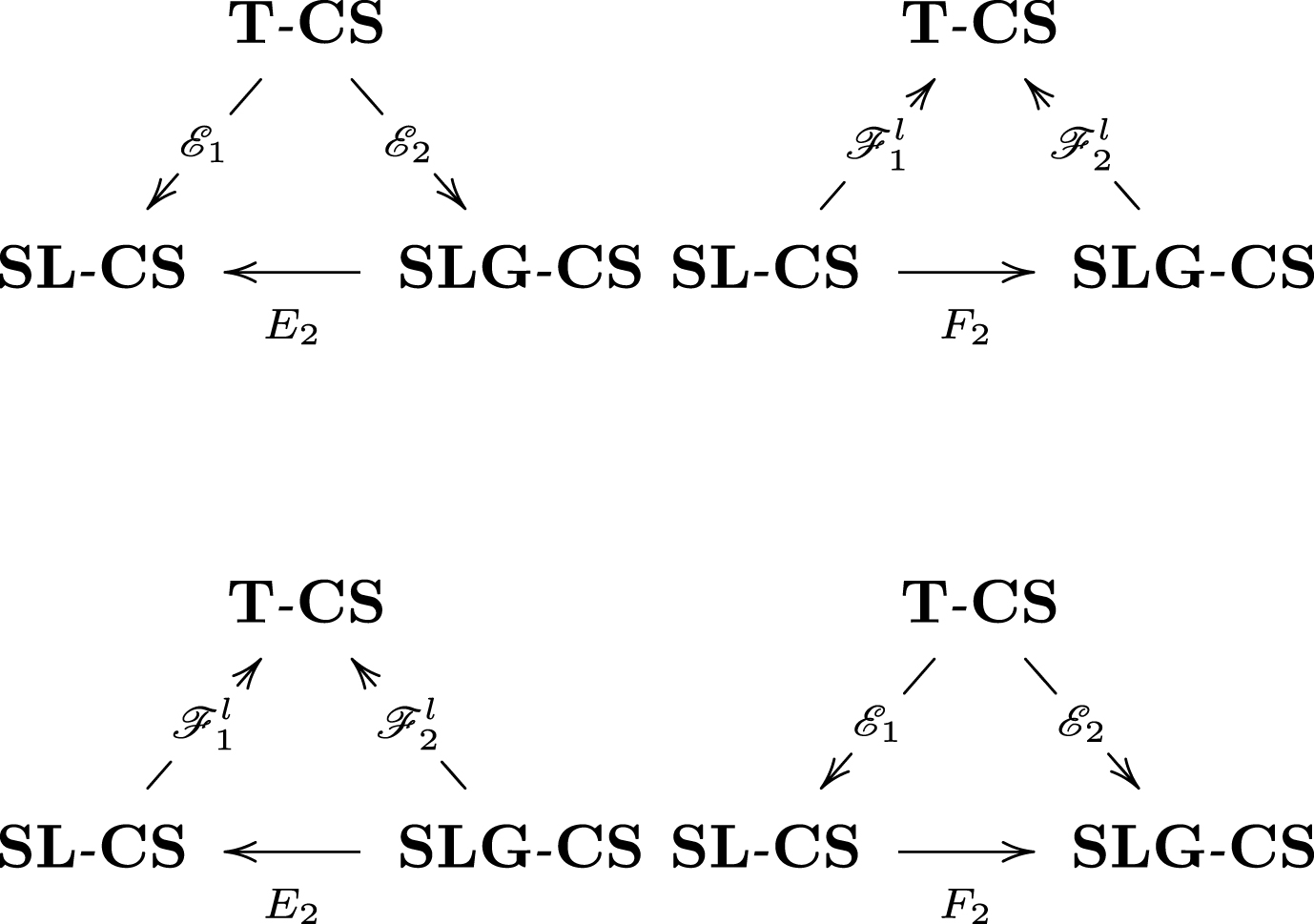
Theorem 3.21. (1) $E_{2} \circ ε_{2} = ε_{1}$ and $ℱ_{2}^{l} \circ F_{2} = ℱ_{1}^{l}; (2) ℱ_{1}^{l} \circ E_{2} = ℱ_{2}^{l}$ and $ε_{2} = F_{2} \circ ε_{1}$ This shows that there exist four commutative diagrams:

Proof. (1) Given (X, q) ∈ T.-CS. Then for any α > ⊥ $\begin{array}{l} F \overset{ℱ_{2}^{l} \circ F_{2} (\bar{q})}{\to} x & \Leftrightarrow ε_{2} (q) ℱ (x) \geq α \\ \Leftrightarrow ε_{2} (q) ℱ (x) = ⊤ \\ \Leftrightarrow \exists F \overset{q}{\to} x s . t . ℱ \geq Λ (F) \\ \Leftrightarrow F \overset{ε_{1} (q) α}{\to} α . \end{array}$

It follows that $E_{2} \circ E_{2} (q) = E_{1} (q)$ .

Given (X, $\bar{q}$ ) ∈ SL-CS. Then $\begin{array}{l} F \overset{ℱ_{2}^{l} \circ F_{2} (\bar{q})}{\to} x \\ \Leftrightarrow & \exists ℱ \in ℱ_{L}^{s} (X) s . t . F_{2} (\bar{q}) ℱ (x) \\ = \lor {α | ℱ \overset{q_{α}}{\to} x} > ⊥, F \supseteq Γ (ℱ) \\ \Leftrightarrow & \exists ℱ \in ℱ_{L}^{s} (X), α > ⊥ s . t . ℱ \overset{q_{α}}{\to} x, \\ F \supseteq Γ (ℱ) \\ \Leftrightarrow & F \overset{ℱ_{1}^{l} (\bar{q})}{\to} x . \end{array}$

It follows that $ℱ_{2}^{l} \circ F_{2} (\bar{q}) = ℱ_{1}^{l} (\bar{q})$ .

(2) Given (X, lim^q) ∈ SLG-CS. Then $\begin{array}{l} F & \overset{ℱ_{1}^{l} \circ E_{2} (\lim^{q})}{\to} x \\ \Leftrightarrow & \exists ℱ \in ℱ_{L}^{s} (X), α > ⊥ s . t . ℱ \overset{E_{2} (\lim^{q}) g_{α}}{\to} x, \\ F \supseteq Γ (ℱ) \\ \Leftrightarrow & \exists ℱ \in ℱ_{L}^{s} (X), α > ⊥ s . t . \lim^{q} ℱ (x) \geq α, \\ F \supseteq Γ (ℱ) \\ \Leftrightarrow & \exists ℱ \in ℱ_{L}^{s} (X), s . t . \lim^{q} ℱ (x) > ⊥, \\ F \supseteq Γ (ℱ) \\ \Leftrightarrow & F \overset{ℱ_{2}^{l} (\lim^{q})}{\to} x . \end{array}$

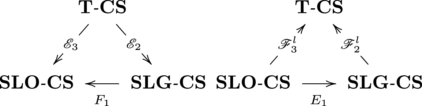
Given (X, q)∈ T-CS. Then $\begin{array}{l} F_{2} \circ ℰ_{1} (q) ℱ (x) = \lor {α | ℱ \overset{ℰ_{1} {(q)}_{α}}{\to} x} \\ = & \lor {α | α > ⊥, ℱ \geq Λ (F), F \overset{q}{\to} x} \\ = & {\begin{array}{l} ⊤, ℱ \geq Λ (F) for some F \overset{q}{\to} x; \\ ⊥, otherwise . \end{array} \\ = & ℰ_{2} (q) ℱ (x) . \end{array}$ □

Theorem 3.22. $F_{1} \circ E_{2} = E_{3}$ and $F_{2}^{l} \circ E_{1} = F_{3}^{l}$ . This shows that there exist two commutative diagrams:

Proof. (1) Given (X, q)∈ T-CS. Then $\begin{array}{l} F_{1} \circ ℰ_{2} (q) ℱ (x) \\ = & \lor {S_{ℱ_{L}^{s} (X)} (G, ℱ) * ℰ_{2} (q) G (x) | G \in ℱ_{L}^{s} (X)} \\ = & \lor {S_{ℱ_{L}^{s} (X)} (G, ℱ) | G \geq Λ (F), F \overset{q}{\to} x} \\ = & \lor {S_{ℱ_{L}^{s} (X)} (Λ (F), ℱ) | F \overset{q}{\to} x} \\ = & ℰ_{3} (q) ℱ (x) . \end{array}$

The equality $F_{2}^{l} \circ E_{1} = F_{3}^{l}$ follows immediately from that $F_{3}^{l}$ is the restriction of $F_{2}^{l}$ on SLO-CS.□

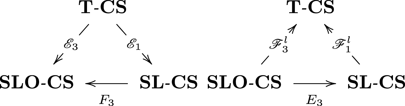
Theorem 3.23. $F_{3} \circ E_{1} = E_{3}$ and $F_{1}^{l} \circ E_{3} = F_{3}^{l}$ . This shows that there exist two commutativediagrams:

Proof. (1) Given (X, q)∈ T-CS. Then $\begin{array}{l} F_{3} \circ ℰ_{1} (q) ℱ (x) \\ = & \lor {α * S_{ℱ_{L}^{s} (X)} (G, ℱ) | G \overset{ℰ_{1} {(q)}_{α}}{\to} x, α \in L} \\ = & \lor {α * S_{ℱ_{L}^{s} (X)} (G, ℱ) | G \geq Λ (F), F \overset{q}{\to} x, α > ⊥} \\ = & \lor {S_{ℱ_{L}^{s} (X)} (Λ (F), ℱ) | F \overset{q}{\to} x} \\ = & ℰ_{3} (q) ℱ (x) . \end{array}$

The equality $F_{1}^{l} \circ E_{3} = F_{3}^{l}$ follows immediately from that $F_{3}^{l}$ is the restriction of $F_{2}^{l}$ on SLO-CS.□

4 Conclusions

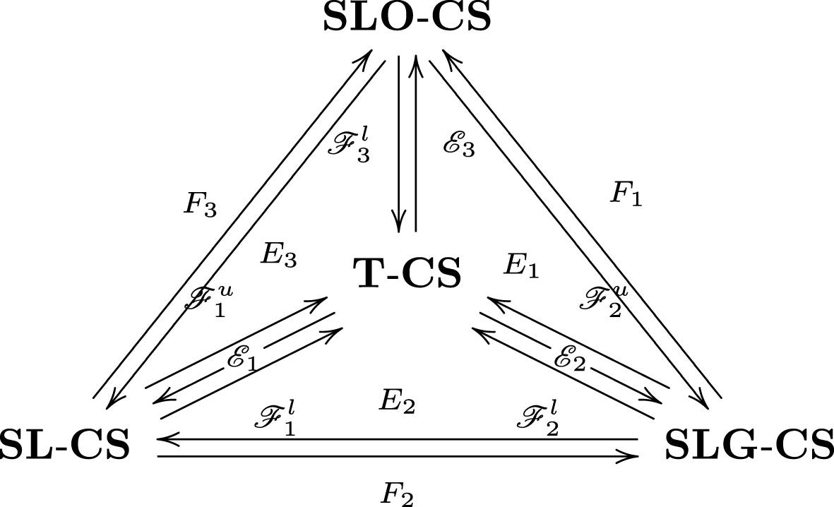
In this paper, a category of modified ⊤-convergence spaces is given and the relationships between this category and three categories of lattice-valued convergence spaces are established. The results can be summarized through the following diagram:

•Five pairs of Galois correspondences: $(E_{i}, F_{i}^{u})$ , $(F_{i}^{l}, E_{i})$ (i = 1, 2), $(E_{3}, F_{3}^{u})$ .

•Three embeddings:

T-CS embedding in SL-CS as both a reflective and coreflective subcategory.

T-CS embedding in SLG-CS as both a reflective and coreflective subcategory.

T-CS embedding in SLO-CS as a coreflective subcategory.

•Eight commutative diagrams.

These commutative diagrams show that as the lattice-valued extensions of category of crisp convergence spaces [33], the considered categories have good compatibility.

Footnotes

Acknowledgments

The author thank the reviewers and the associated editor Prof. Esteban Indurain for their valuable comments and suggestions. This work is supported by National Natural Science Foundation of China (No. 11501278, 11471152).

References

Adámek

, Herrlich

, Strecker

G.E.

Abstract and Concrete Categories, Wiley, New York, 1990.

Bělohlávek

, Fuzzy Relational Systems: Foundations and Principles, Kluwer Academic Publishers, New York, 2002.

Boustique

and Richardson

, A note on regularity, Fuzzy Sets and Systems 162 (2011), 64–66.

Fang

J.M.

, Stratified L-ordered convergence structures, Fuzzy Sets and Systems 161 (2010), 2130–2149.

Fang

J.M.

and Yue

Y.L.

, T-diagonal conditions and Continuous extension theorem, Fuzzy Sets and Systems 321 (2017), 73–89.

Flores

P.V.

, Mohapatra

R.N.

and Richardson

, Lattice-valued spaces: Fuzzy convergence, Fuzzy Sets and Systems 157 (2006), 2706–2714.

Flores

P.V.

and Richardson

, Lattice-valued convergence: Diagonal axioms, Fuzzy Sets and Systems 159 (2008), 2520–2528.

Gao

X.Y.

, Pang

and Yang

X.F.

, Extensional L-fuzzy Q-convergence structures, Journal of Intelligent and Fuzzy Systems 31(3) (2016), 1701–1708.

Gierz

, Hofmann

K.H.

, Keimel

, Lawson

J.D.

, Mislove

M.W.

, Scott

D.S.

Continuous Lattices and Domains, Cambridge University Press, Cambridge, 2003.

10.

Gutiérrez

, García, On stratified L-valued filters induced by T-filters, Fuzzy Sets and Systems 157 (2006), 813–819.

11.

Höhle

, Šostak

Axiomatic foundations of fixed-basis fuzzy topology, Höhel

, Rodabaugh

S.E.

(Eds.), Mathematics of Fuzzy Sets: Logic, Toology and Measure Theory, The Handbooks of Fuzzy Sets Series, Vol. 3, Kluwer Academic Publishers, Boston, Dordrecht, London, 1999, pp. 123–273.

12.

and Li

J.Q.

, The entropy and similarity measure of interval valued intuitionistic fuzzy sets and their relationship, International Journal of Fuzzy Systems 15(3) (2013), 279–288.

13.

Jäger

, A category of L-fuzzy convergence spaces, Quaestiones Mathematicae 24 (2001), 501–517.

14.

Jäger

, Gähler’s neighbourhood condition for lattice-valued convergence spaces, Fuzzy Sets and Systems 204 (2012), 27–39.

15.

Jäger

, Stratified LMN-convergence tower spaces, Fuzzy Sets and Systems, Fuzzy Sets and Systems 282 (2016), 62–73.

16.

Jäger

, Connectedness and local connectedness for latticevalued convergence spaces, Fuzzy Sets and Systems 300 (2016), 134–146.

17.

Jin

and Li

L.Q.

, One-axiom characterizations on lattice-valued closure (interior) operators, Journal of Intelligent and Fuzzy Systems 31 (2016), 1679–1688.

18.

Jin

, Li

L.Q.

, Lv

Y.R.

et al., Connectedness for lattice-valued subsets in lattice-valued convergence spaces, Quaestiones Mathematicae, 10.2989/16073606.2018.1441920

19.

Jin

, Li

L.Q.

and Meng

G.W.

, On the relationships between types of L-convergence spaces, Iranian Journal of Fuzzy Systems 1 (2016), 93–103.

20.

L.Q.

, On the category of enriched (L, M)-convex spaces, Journal of Intelligent and Fuzzy Systems 33 (2017), 3209–3216.

21.

L.Q.

and Jin

, On adjunctions between Lim, S)-Top, and S)-Lim, Fuzzy Sets and Systems 182 (2011), 66–78.

22.

L.Q.

and Jin

, On stratified}-convergence spaces: Pretopological axioms and diagonal axioms, Fuzzy Sets and Systems 204 (2012), 40–52.

23.

L.Q.

and Jin

, p-Topologicalness and p-Regularity for latticevalued convergence spaces, Fuzzy Sets and Systems 238 (2014), 26–45.

24.

L.Q.

, Jin

and Hu

, On stratified L-convergence spaces: ’s diagonal axiom, Fischer’s Fuzzy Sets and Systems 267 (2015), 31–40.

25.

L.Q.

, Jin

and Hu

, Lattice-valued convergence associated with CNS spaces, Fuzzy Sets and Systems (2018), 10.1016/j.fss.2018.05.023

26.

L.Q.

, Jin

, Hu

and Zhao

F.F.

, The axiomatic characterizations on L-fuzzy covering-based approximation operators, International Journal of General Systems 46 (2017), 332–353.

27.

L.Q.

, Jin

, Meng

G.W.

et al. The lower and upper p-topological (p-regular) modifications for lattice-valued convergence spaces, Fuzzy Sets and Systems 282 (2016), 47–61.

28.

L.Q.

and Li

Q.G.

, On enriched L-topologies: Base and subbase, Journal of Intelligent and Fuzzy Systems 28 (2015), 2423–2432.

29.

L.Q.

and Li

Q.G.

, A new regularity (p-regularity) of stratified-generalized convergence spaces, Journal of Computational Analysis and Applications 2 (2016), 307–318.

30.

Orpen

and Jäger

, Lattice-valued convergence spaces: Extending the lattices context, Fuzzy Sets and Systems 190 (2012), 1–20.

31.

Pang

and Zhao

, L-fuzzy N-convergence structures, Journal of Intelligent and Fuzzy Systems 30(5) (2016), 3033–3043.

32.

Pang

and Zhao

, Several types of enriched (L,M)-fuzzy convergence spaces, Fuzzy Sets and Systems 321 (2017), 55–72.

33.

Preuss

, Fundations of Topology, Kluwer Academic Publishers, London, 2002.

34.

Qiu

and Fang

J.M.

, The category of all T-convergence spaces and its cartesian-closedness, Iranian Journal of Fuzzy Systems 14(3) (2017), 121–138.

35.

Reid

and Richardson

, Connecting T and Lattice-Valued Convergences, Iranian Journal of Fuzzy Systems (in press).

36.

Rosenthal

K.I.

, Quantales and Their Applications, Longman Scientific & Technical, 1990.

37.

Sun

S.B.

, Xiu

Z.Y.

and Li

Q.L.

, On fuzzifying matroids: Dual matroids and spanning, Journal of Intelligent and Fuzzy Systems 3 (2015), 1435–1440.

38.

Yao

, On many-valued stratified L-fuzzy convergence spaces, Fuzzy Sets and Systems 159 (2008), 2503–2519.

39.

Zhang

D.X.

, An enriched category approach to many valued topology, Fuzzy Sets and Systems 158 (2007), 349–366.

40.

Zhang

X.F.

, Li

L.Q.

and Meng

G.W.

, A modified uncertain entailment model, Journal of Intelligent and Fuzzy Systems 27(1) (2014), 549–553.

41.

Zhao

F.F.

, Jin

and Li

L.Q.

, The axiomatic characterizations on L-generalized fuzzy neighborhood system-based approximation operators, International Journal of General Systems 47(2) (2018), 155–173.