Geometric picture fuzzy numbers and three-dimensional copulas with the non-linear programming approach

Abstract

This study presents a possible relationship between two main objects, which are three-dimensional copulas (3D-Cs) and geometric picture fuzzy numbers (GPFNs). This opens up a potential field for future studies for these two objects that three-dimensional copulas can become useful tools for handling uncertainty information in the form of a picture fuzzy set (PFS). Specifically, we define a GPFN as a base element of the PFS and a defined domain of three-dimensional copulas that contains a set of GPFNs, then we show some examples of three-dimensional copulas identified on this domain. In this framework, we present the theorems related to these two objects. At the same time, we provide some examples for three-dimensional semi-copulas, three-dimensional quasi-copulas, and three-dimensional empirical copulas defined on D, which is a defined domain of a three-dimensional copula and contains a set of GPFNs $D_{g}^{*} .$ In addition, we also introduce a new approach to non-linear programming problems.

Keywords

Three-dimensional distribution functions,three-dimensional copulas (3D-Cs)geometric picture fuzzy numbers (GPFNs)additional set of geometric picture fuzzy numbers (Ad-GPFNs)non-linear programming approach

1 Introduction

Since 1951, Frechet studied distribution functions of random variables defined on the probability space. He studied the following problem: Given d random variables, defined the marginals F₁, F₂, . . . , F_d and an joint distribution function H (F₁, F₂, . . . , F_d) . The problem is hence related to the determination of random sets X₁, X₂, . . . , X_d (see Frechet [15], 1951). Many studies about this problem were conducted by Feron for three-dimensional distribution functions (see [14]1956), by Frechet for multidimensional distribution functions (see [16],1956), by Marshall and Olkin for generalized bivariate exponential distribution (see [24], 1996). The marginals and joint distribution functions can be applied to statistical modelling (see [6], 2003).

The history of copulas began in 1959 with Sklar’s Theorem [30]. The proof of this theorem was not given in 1959. It’s was provided by Sklar in 1973 [31]. The copulas are the mathematical tool for combining for the joint distribution functions. The most results concerning copulas were obtained in:

the statistical community by Scheizer and Wolff (see [29],1981);

the finance by Genest et all (see [17], 2009) and Jaworski et all (see [20], 2013);

the enviromental scince by Genest and Favre (see [18], 2007) and Salvadori (see [28], 2007);

the biostatistics by Hougaard (see [19], 2000) and Song (see [35], 2007);

the decision scince by Clemen and Reilly (see [5], 1999);

the machine learning by Elidan (see [13], 2013);

Nowadays, the interest in copulas is investigated in both tend the basis on copulas and the applications to the many fields in finance and risk management.

The concept of fuzzy sets (FSs) was introduced in 1965 by L.A. Zadeh [42], a lot of research was investigated to make the foundations of this new notion, in algebraic logic. The t-norms started with Menger (see [25], 1985), whose idea was to construct metric spaces when probability distribution functions (pDFs) were used to describe the distance between elements. The t-norms are played an important role in the Fuzzy set theory. Almost all of the studies of t-norms based operations on fuzzy numbers. The t-norms and t-conorms are the mathematical operators for combining information by Dubois, Prade (see [11], 1981), and Klement (see [21], 1982). The properties of t-norms for possible use in the development of intelligent systems were studied by Bonissone (see [3], 1985). The t-norms have also been used in the design of fuzzy controllers, in modeling, and in the decision marking problems, such that satisfy some properties of the copulas (can see in [30]).

In 2014, Cuong [7] introduced the concept of picture fuzzy sets (PFS), which is a generalization of the traditional fuzzy sets (FS) and the intuitionistic fuzzy sets (IFS). Then, some operations on PFS with some properties are considered and the basic preliminaries of PFS Theory are presented [8]. In literature, the results on PFS connectives almost have algebraic, logical operations [36], and fuzzy clustering [33]. Recently, L.H. Son [34] proposed a generalized picture distance measure and integrate it into a novel hierarchical picture fuzzy clustering method. Based on the idea of "picture fuzzy sets", we define the concept of the geometric picture fuzzy numbers as an ordered set which consists of a membership degree, a neutral membership degree, and a non-membership degree. Similar to the intuitionistic fuzzy numbers, the geometric picture fuzzy numbers have a great potential for application in multi-criteria decision making (MCDM) methods. MCDM methods are a tool to reduce the subjectivity of decision making by creating a series of filter options and helping to make a selection out of complex alternatives. Many interesting studies have been done, for example, Badi and his colleagues [4] used a new method (called combinative distance-based assessment - CODAS) to handle MCDM problems for a steelmaking company in Libya, Mukhametzyanov and Pamucar [23] provided a model for result consistency evaluation of MCDM methods and presented the results of an analysis of the sensitivity of decision-making based on the rank methods, Liu et al. [22] presented a new multicriteria model of the selection that significantly influences its further flow is decision-making about the choice of the most favorable transport provider. Wang et al. [37] formulated a hybrid fuzzy multi-criteria decision-making framework, which not only considers the interrelationship among criteria but also considers the decision-maker’s bounded rationality and behavioural psychology, with picture fuzzy information to rank the risk factors of energy performance contracting projects. Zhang et al. [41] presented the picture fuzzy evaluation based on distance from the average solution (EDAS) model for multiple-criteria group decision-making based on the traditional EDAS model and some fundamental theories of picture 2-tuple linguistic numbers. R. Wang et al. [38] studied on multiple attribute decision-making (MADM) problems with picture fuzzy numbers information and adopted the PFWMM and picture fuzzy weighted dual Muirhead mean operators to build a decision-making model to handle picture fuzzy MADM problems. Wei et al. [39] used the q-rung orthopair fuzzy weighted dual Maclaurin symmetric mean operator to develop an approach to solve the q-rung orthopair fuzzy multiple-attribute decision-making problems. G. Wei and Z. Zhang [40] utilized power aggregation operators and Bonferroni mean to develop some single-valued neutrosophic Bonferroni power aggregation operators and single-valued neutrosophic geometric Bonferroni power aggregation operators and used the SVNWBPM and SVNWGBPM operators to solve the single-valued neutrosophic multiple-attribute decision-making problems. Peng [27] utilized induced ordered weighted geometric operator to develop picture fuzzy induced ordered weighted geometric operators and used the picture fuzzy induced ordered weighted geometric to solve the picture fuzzy multiple attribute decision-making problems.

If t-norms (see [25]) are the mathematical tool for combining membership degrees of fuzzy sets, the copulas (see [30]) are the mathematical tool for illustration of probability marginals and joint distribution functions. Both the distribution functions and the copulas have similarities: there are copulas are distribution functions and vice versa. Many problems in the financial and economic fields, such as risk management, derivative valuation, stock market options, stock portfolio optimization, market spread, and financial, are based on the investigation of several important function classes: the marginals, the joint distribution functions (jDFs) with copula-like structure (Copulas), logical operations or t-norms (t-N) and more recently intuitionistic fuzzy numbers (IFNs).

In recent results, Dolati and his colleagues [9] introduced a new family of fuzzy implication operators which are based on the conditional version of a copula function. In [2], the authors introduced a method of defining commutative semicopulas from fuzzy negations. Most recently, Sun and his colleagues [32] proposed a fuzzy copula model to recognize the possibilistic uncertainty of wind speed correlation. As we know, the copula theory, the fuzzy theory or the Picture fuzzy theory have developed independently of each other. Some cited above shows that many researchers began to consider the relationship between the copula theory and the fuzzy theory, but the relationship between the copula theory and the Picture fuzzy theory is very new. In 2004, Deschrijver and his colleagues ([10]) built the t-norms and t-conorms on L^* (it is the place in which the intuitionistic fuzzy sets take the value and this value is the intuitionistic fuzzy numbers). From the visual relationships of t-norms and copula. Along with some of the results built the t-norms and t-conorms on L^* (can see in [10]). We notice that the problem of developing the copula on $D_{g}^{*}$ (it is the place in which the picture fuzzy sets take the value and this value is the geometric picture fuzzy number) is possible. To do this, we provide a few theorems and examples about the existence of some three-dimensional copulas that we can use them to perform calculations with picture fuzzy data based on the idea of geometric picture fuzzy numbers. Our contributions are as follows: Firstly, we give definitions of the geometric picture fuzzy numbers (GPFN), the set of GPFNs, which is denoted by $D_{g}^{*}$ , and the additional set of GPFNs, which is denoted by ${\bar{D}}_{g}^{*} .$ Secondly, we define a joint distribution function for three terms of a GPFN as a copula with a defined domain, which is $D = D_{g}^{*} \cup {\bar{D}}_{g}^{*} .$ A theorem on the existence of this copula is also presented. Thirdly, we provide practical examples of three-dimensional semi-copulas, three-dimensional quasi-copulas, and three-dimensional copulas on $D_{g}^{*},$ ${\bar{D}}_{g}^{*},$ and D, respectively. Finally, we introduce a new approach to non-linear programming. The main idea of this approach is to replace the objective function of non-linear programming by a copula with a defined domain D or with a semi-copula with a defined domain $D_{g}^{*},$ which is the place in which the picture fuzzy sets take the value and this value is the GPFNs. This makes it possible to study non-linear programming based on picture fuzzy information through the idea of GPFNs.

This paper includes: In section 2, we recall some notations and concepts presented in detail in series of researches about marginals, three-dimensional joint distribution functions (3D-jDFs), semi-copulas (S-Copulas), quasi-copulas (Q-Copulas), three-dimensional copulas (3D-Cs). At the same time, we also present the concept of a geometric picture fuzzy numbers (GPFNs), the set of the GPFNs and the additional set of GPFNs. In section 3, we present a few theorems and examples about the existence of some three-dimensional (3D) semi-copulas, 3D-quasi-copulas, and 3D-copulas. In section 4, we introduce a non-linear programming approach.

2 Preliminaries and notation

We recall some notations and concepts presented in detail in a series of researches about three-dimensional joint distribution functions (3-jDFs), three-dimensional copulas (3D-Cs), and the picture fuzzy sets (PFSs).

2.1 The three-dimensional distribution functions

Let $(Ω, F, P)$ be a probability space. The sets A, B, C ∈ Ω with probabilities P (A) , P (B) , P (C) we have

$\begin{matrix} max {P (A) + P (B) + P (C) - 2, 0} ⩽ P (A \cap B \cap C) \\ ⩽ min {P (A), P (B), P (C)} . \end{matrix}$ (1)

Definition 1. (see [12] for d random events) Let be three random variables X₁, X₂, X₃, then three random events A = {X₁ < x₁} , B = {X₂ < x₂} and C = {X₃ < x₃} define their marginals:

$\begin{matrix} F_{X_{1}} (x_{1}) = P (X_{1} < x_{1}), F_{X_{2}} (x_{2}) = P (X_{2} < x_{2}), \\ F_{X_{3}} (x_{3}) = P (X_{3} < x_{3}) \end{matrix}$ (2) and the joint distribution function of X₁, X₂, X₃ :

$\begin{matrix} H (x_{1}, x_{2}, x_{3}) = F_{X_{1} X_{2} X_{3}} (x_{1}, x_{2}, x_{3}) \\ = P ({X_{1} < x_{1}} \cap {X_{2} < x_{2}} \cap {X_{3} < x_{3}}) . \end{matrix}$ (3)

2.2 The three-dimensional copulas

Definition 2. A function Con : [0, 1] × [0, 1] × [0, 1] → [0, 1] is called a three dimensional conjunctor if for all x₁, x₂, x₃ ∈ [0, 1] the following axioms are satisfied:

Con (0, x₂, x₃) = Con (x₁, 0, x₃) = Con (x₁, x₂, 0) =0 ;

Con (1, 1, 1) =1 .

Definition 3. [26] A three-dimensional semi-copula (3D-SCs) is a conjunctor C₁ : [0, 1] × [0, 1] × [0, 1] → [0, 1] with 1 as neutral element, that for all x₁, x₂, x₃ ∈ [0, 1] satisfies:

Con (0, x₂, x₃) = Con (x₁, 0, x₃) = Con (x₁, x₂, 0) =0 ;

C₁ (1, 1, 1) =1 ;

C₁ (x₁, 1, 1) = C₁ (1, x₁, 1) = C₁ (1, 1, x₁) = x₁ .

Definition 4. A three-dimensional quasi-copula (3D-QCs) is a 3D-SCs C₂ : [0, 1] × [0, 1] × [0, 1] → [0, 1] with 1-Lipschitz in both variables, that for all x₁, x₂, x₃ ∈ [0, 1] satisfies:

C₂ (x₁, 0, 0) = C₂ (0, x₂, 0) = C₂ (0, 0, x₃) =0 ;

C₂ (1, 1, 1) =1 ;

C₂ (x_k, 1, 1) = C₂ (1, x_k, 1) = C₂ (1, 1, x_k) = x_k at lear index k ∈ {1, 2, 3} .

Definition 5. A three-dimensional function f : [0, 1] × [0, 1] × [0, 1] → [0, 1] , which denotes by f (x₁, x₂, x₃) , is called 3D-increasing on [0, 1] if for x_k, y_k ∈ [0, 1] with x_k ⩽ y_k, k ∈ {1, 2, 3} , satisfies the following condition: $\begin{matrix} f (x_{1}, x_{2}, x_{3}) - f (x_{1}, x_{2}, y_{3}) - f (x_{1}, y_{2}, x_{3}) \\ - f (y_{1}, x_{2}, x_{3}) + f (y_{1}, y_{2}, y_{3}) \geq 0 . \end{matrix}$

We can see a description of f (x₁, x₂, x₃) is 3D-increasing on [0, 1] (in Figure 1). Assume that the volume of the boxes in Figure 1 corresponds to the value of the functions as follows:

Fig. 1

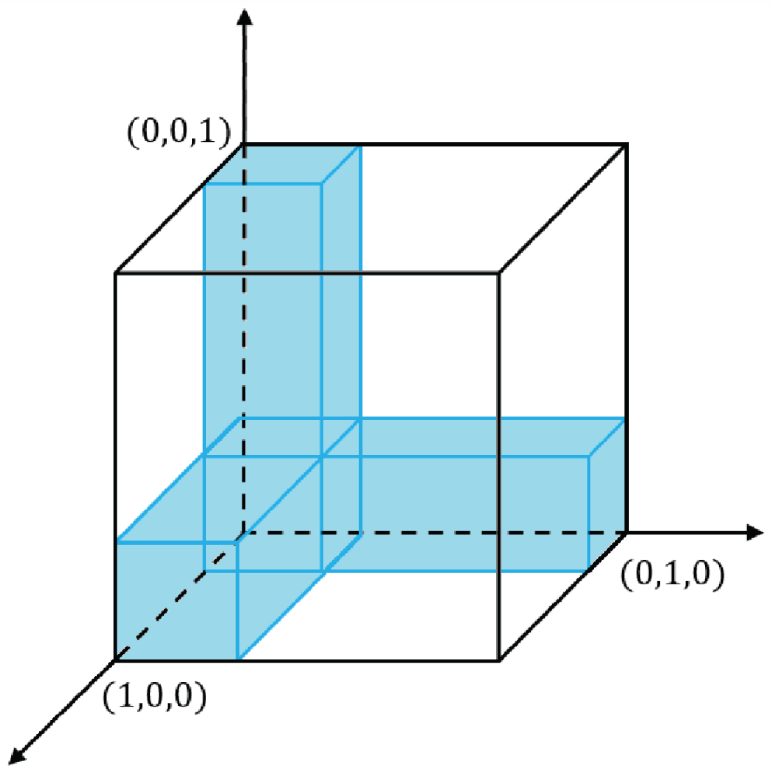
A description of f (x₁, x₂, x₃) is 3D-increasing on [0, 1] .

B_x (x₁, x₂, x₃) = x₁x₂x₃ = f (x₁, x₂, x₃) ;

B_y (y₁, y₂, y₃) = y₁y₂y₃ = f (y₁, y₂, y₃) ;

B_{y
₁} (y₁ - x₁, x₂, x₃) = (y₁ - x₁) x₂x₃ = f (y₁ - x₁, x₂, x₃) ;

B_{y
₂} (x₁, y₂ - x₂, x₃) = x₁ (y₂ - x₂) x₃ = f (x₁, y₂ - x₂, x₃) ;

B_{y
₃} (x₁, x₂, y₃ - x₃) = x₁x₂ (y₃ - x₃) = f (x₁, x₂, y₃ - x₃) ,

such that, we have

$\begin{matrix} B_{x} (x_{1}, x_{2}, x_{3}) - B_{y_{3}} (x_{1}, x_{2}, y_{3} - x_{3}) - B_{y_{2}} (x_{1}, y_{2} \\ - x_{2}, x_{3}) - B_{y_{1}} (y_{1} - x_{1}, x_{2}, x_{3}) + B_{y} (y_{1}, y_{2}, y_{3}) \geq 0 . \end{matrix}$

Definition 6. A three-dimensional copula (3D-Cs) is a function C : [0, 1] × [0, 1] × [0, 1] → [0, 1] denoted by C (x₁, x₂, x₃) , which satisfies the following conditions:

[a/] C (x₁, x₂, x₃) =0 if x_k = 0 at index k∈ {1, 2, 3} ; em [b/] C (1, 1, 1) =1 ; em [c/] C (x_k, 1, 1) = C (1, x_k, 1) = C (1, 1, x_k) = x_k at index k∈ {1, 2, 3} ; em [d/] C (x₁, x₂, x₃) is 3D-increasing on [0, 1] .

2.3 The geometric picture fuzzy numbers

We recall some notations and concepts presented in detail in a series of researches about fuzzy sets and its extended (see [1 , 42]).

Definition 7. [42] Let U be a universe set, then a fuzzy set $C = {(u, μ_{C} (u)) | u \in U}$ that is characterized by a membership function: $μ_{C} : U \to [0, 1]$ (4) and define the membership degree of a element u ∈ U such that 0 ≤ μ_C (u) ≤1.

In [1], Atanassov introduced the concept of intuitionistic fuzzy set (IFS), characterized by a membership function and a non-membership function, which is a generalization of fuzzy set.

Definition 8. [1] Let U be a universe set, then an intuitionistic fuzzy set $B = {(u, μ_{B} (u), ν_{B} (u)) | u \in U}$ that is characterized by a membership function: $μ_{B} : U \to [0, 1],$ (5) and by a non-membership function: $ν_{B} : U \to [0, 1],$ (6) and define the membership degree μ_B (u) and the non-membership degree ν_B (u) of element u ∈ U, respectively, such that 0 ≤ μ_B (u) + ν_B (u) ≤1 .

In 2014, Cuong [7] introduced the concept of picture fuzzy set (PFSs), characterized by a membership function, a neutral membership function and a non-membership function, which is a direct extension of the fuzzy sets (FS) and the intuitionistic fuzzy sets (IFS).

Definition 9. [7] Let U be a universe set, then a picture fuzzy set $A = {(u, μ_{A} (u), η_{A} (u), ν_{A} (u)) | u \in U}$ that is characterized by membership function: $μ_{A} : U \to [0, 1],$ (7) by neutral membership function: $η_{A} : U \to [0, 1],$ (8) and by non-membership function: $ν_{A} : U \to [0, 1],$ (9) and define a membership degree μ_A (u), a neutral membership degree η_A (u) and a non-membership degree ν_A (u) of element u ∈ U, respectively, such that 0 ⩽ μ_A (u) + η_A (u) + ν_A (u) ⩽1 .

From Definition 9, let A ={ (u, μ_A (u) , η_A (u) , ν_A (u)) |u ∈ U } be a picture fuzzy set with 0 ⩽ μ_A (u) + η_A (u) + ν_A (u) ⩽1, putting x = (x₁, x₂, x₃) = (μ_A (u) , η_A (u) , ν_A (u)) then we have a box $B_{x} = {(v, w, u) | 0 ⩽ v ⩽ x_{1}, 0 ⩽ w ⩽ x_{2}, 0 ⩽ u ⩽ x_{3}} .$ and each element x = (x₁, x₂, x₃) ∈ [0, 1] ³ with 0 ⩽ x₁ + x₂ + x₃ ⩽ 1 is called a geometric picture fuzzy number (GPFN).

Definition 10. Let $D_{g}^{*}$ be denoted a set of geometric picture fuzzy numbers (GPFNs) as follows:

$D_{g}^{*} = {x = (x_{1}, x_{2}, x_{3}) \in [0, 1]^{3} | 0 ⩽ x_{1} + x_{2} + x_{3} ⩽ 1},$ (10)

where x₁ corresponding to membership degree, x₂ corresponding to neutral membership degree and x₃ corresponding to non-membership degree and each element $x \in D_{g}^{*}$ is called a geometric picture fuzzy number (GPFN).

Definition 11. We denote that

$θ = (0, 0, 0) \in D_{g}^{*}$ is called a zero element of $D_{g}^{*} .$

If $x = (x_{1}, x_{2}, x_{3}) \in D_{g}^{*}$ then $\bar{x} = (x_{3}, x_{2}, x_{1}) \in D_{g}^{*}$ is called a reverse element of $x \in D_{g}^{*} .$

D_{g}^{*}

is called a set of geometric picture fuzzy numbers (GPFNs), whose graph shown in Figure 2, 3.

Fig. 2

Geometric interpretation of $D_{g}^{*}$ .

Fig. 3

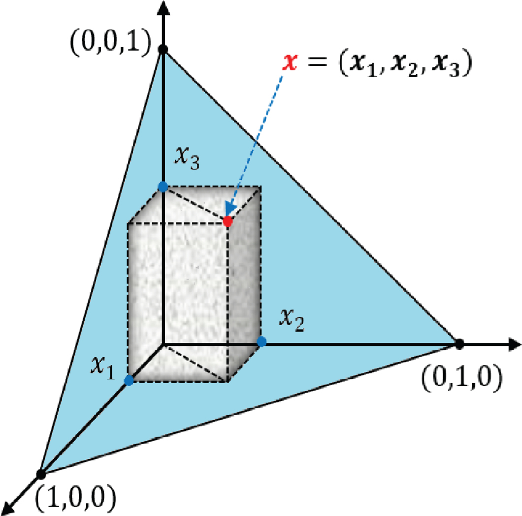
The box B_x and a geometric interpretation of geometric picture fuzzy number (GPFN) x = (x₁, x₂, x₃) in $D_{g}^{*}$ .

Definition 12. We denote ${\bar{D}}_{g}^{*} = {x = (x_{1}, x_{2}, x_{3}) \in [0, 1]^{3} | x_{1} + x_{2} + x_{3} > 1},$ (11) that is called an additional set of geometric picture fuzzy numbers (Ad-GPFNs), whose graph shown in the ${\bar{D}}_{g}^{*}$ by Figure 4.

Fig. 4

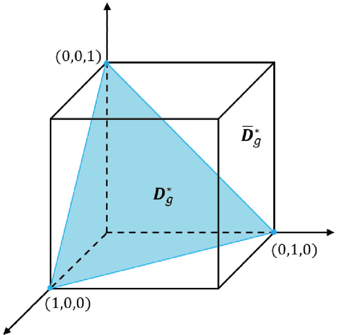
Picture description of the additional set of geometric picture fuzzy numbers (Ad-GPFNs) ${\bar{D}}_{g}^{*}$ .

3 Main result

Theorem 1. Let x = (x₁, x₂, x₃) be a GPFN of a picture fuzzy set A and a function C : [0, 1] × [0, 1] × [0, 1] → [0, 1] be a three-dimensional copula. Putting the marginals F₁ (x₁) = x₁, F₂ (x₂) = x₂, and F₃ (x₃) = x₃ with a joint membership function F (x₁, x₂, x₃) = C (x₁, x₂, x₃) , then we have $\begin{matrix} max {x_{1} + x_{2} + x_{3} - 2, 0} \\ ⩽ F (x_{1}, x_{2}, x_{3}) ⩽ min {x_{1}, x_{2}, x_{3}} . \end{matrix}$

Proof. The result of this theorem is deduced from the property of the copula. Indeed, in copula theory, we have $W (x_{1}, x_{2}, x_{3}) \leq C (x_{1}, x_{2}, x_{3}) \leq M (x_{1}, x_{2}, x_{3})$ where W (x₁, x₂, x₃) = max{ x₁ + x₂ + x₃ - 2, 0 } and M (x₁, x₂, x₃) = min { x₁, x₂, x₃ } . Therefore, we get $\begin{matrix} max {x_{1} + x_{2} + x_{3} - 2, 0} \\ ⩽ F (x_{1}, x_{2}, x_{3}) ⩽ min {x_{1}, x_{2}, x_{3}} . \end{matrix}$

Remark 1. By the Definitions 6, 11 and 12 we have the defined domain of 3D-copulas: $D = D_{g}^{*} \cup {\bar{D}}_{g}^{*},$ where C : D → [0, 1] such that at special point (0, 0, 0) the 3D-Cs C (0, 0, 0) =0, and at (1, 1, 1) the 3D-Cs C (1, 1, 1) =1 .

Theorem 2. Let $x = (x_{1}, x_{2}, x_{3}) \in D_{g}^{*}$ with 0 ⩽ x₁ + x₂ + x₃ ⩽ 1, then there exist some following 3D-semi-copulas:

C₁ (x₁, x₂, x₃) = x₁ . x₂ . x₃ ;

$C_{1} (x_{1}, x_{2}, x_{3}) = x_{1}^{2} . x_{2} . x_{3};$

$C_{1} (x_{1}, x_{2}, x_{3}) = x_{1} . x_{2}^{2} . x_{3};$

$C_{1} (x_{1}, x_{2}, x_{3}) = x_{1} . x_{2} . x_{3}^{2};$

$C_{1} (x_{1}, x_{2}, x_{3}) = x_{1}^{2} . x_{2}^{2} . x_{3};$

$C_{1} (x_{1}, x_{2}, x_{3}) = x_{1}^{2} . x_{2} . x_{3}^{2};$

$C_{1} (x_{1}, x_{2}, x_{3}) = x_{1} . x_{2}^{2} . x_{3}^{2};$

$C_{1} (x_{1}, x_{2}, x_{3}) = x_{1}^{2} . x_{2}^{2} x_{3}^{2} .$

Proof. We will review the terms of the 3D-semi-copula in Definition 3:

C₁ (x₁, x₂, x₃) is 3D-Conjunctor, which means that it is a function Con : [0, 1] × [0, 1] × [0, 1] → [0, 1] with all x₁, x₂, x₃ ∈ [0, 1] the following axioms are satisfied

$C_{1} (0, x_{2}, x_{3}) = C_{1} (x_{1}, 0, x_{3}) = C_{1} (x_{1}, x_{2}, 0) = 0;$ and $C_{1} (1, 1, 1) = 1;$

C₁ (1, x₂, 1) = x₂ and C₁ (x₁, 1, 1) = x₁, C₁ (1, 1, x₃,) = x₃, with 1 as a neutral element.

By direct inspection, we see that all kinds of C₁ (x₁, x₂, x₃) in the Theorem 2 are the 3D-semi-copulas.

Theorem 3. Let x = (x₁, x₂, x₃) ∈ D . If there exist the 3D-semi-copulas C₁ (x₁, x₂, x₃) with $x = (x_{1}, x_{2}, x_{3}) \in D_{g}^{*}$ in Theorem 2, then there exist some following 3D-quasi-copulas on the additional set of geometric picture fuzzy numbers ${\bar{D}}_{g}^{*}$ with x₁ + x₂ + x₃ > 1 : With 1 < x₁ + x₂ + x₃ ⩽ 2 :

C₂ (x₁, x₂, x₃) = x₁+ x₂ + x₃ - 1 + C₁ (1 - x₁, 1 - x₂, 1 - x₃) ;

C₂ (x₁, x₂, x₃) = x₁+ x₂ + x₃ - 1 + C₁ (1 - x₁, 1 - x₃, 1 - x₂) ;

C₂ (x₁, x₂, x₃) = x₁+ x₂ + x₃ - 1 + C₁ (1 - x₂, 1 - x₁, 1 - x₃) ;

C₂ (x₁, x₂, x₃) = x₁+ x₂ + x₃ - 1 + C₁ (1 - x₂, 1 - x₃, 1 - x₁) ;

C₂ (x₁, x₂, x₃) = x₁+ x₂ + x₃ - 1 + C₁ (1 - x₃, 1 - x₁, 1 - x₂) ;

C₂ (x₁, x₂, x₃) = x₁ + x₂ + x₃ - 1 + C₁ (1 - x₃, 1 - x₂, 1 - x₁) .

With x₁ + x₂ + x₃ > 2 :

C₂ (x₁, x₂, x₃) = x₁+ x₂ + x₃ - 2 + C₁ (1 - x₁, 1 - x₂, 1 - x₃) ;

C₂ (x₁, x₂, x₃) = x₁+ x₂ + x₃ - 2 + C₁ (1 - x₁, 1 - x₃, 1 - x₂) ;

C₂ (x₁, x₂, x₃) = x₁+ x₂ + x₃ - 2 + C₁ (1 - x₂, 1 - x₁, 1 - x₃) ;

C₂ (x₁, x₂, x₃) = x₁+ x₂ + x₃ - 2 + C₁ (1 - x₂, 1 - x₃, 1 - x₁) ;

C₂ (x₁, x₂, x₃) = x₁+ x₂ + x₃ - 2 + C₁ (1 - x₃, 1 - x₁, 1 - x₂) ;

C₂ (x₁, x₂, x₃) = x₁ + x₂ + x₃ - 2 + C₁ (1 - x₃, 1 - x₂, 1 - x₁) .

Proof. Similar to proof of Theorem 2, we will review the terms of the 3D-quasi-copula in Definition 4:

C₁ (x₁, x₂, x₃) is 3D-semi-copula in $D_{g}^{*}$ , that is satisfied the conditions of Theorem 2.

C₂ (x₁, x₂, x₃) that is 1-Lipschitz in both variables.

By direct inspection, we see that all kinds of C₂ (x₁, x₂, x₃) in the Theorem 3 are the 3D-quasi-copulas.

Theorem 4. (on a 3D-empirical-copula) Let x = (x₁, x₂, x₃) ∈ D . If there exist the 3D-semi-copulas C₁ (x₁, x₂, x₃) with $x = (x_{1}, x_{2}, x_{3}) \in D_{g}^{*}$ as in Theorem 2 and the 3D-quasi-copulas C₂ (x₁, x₂, x₃) with $x = (x_{1}, x_{2}, x_{3}) \in {\bar{D}}_{g}^{*}$ as in Theorem 3, then we have an 3D-empirical-copula, which denotes by: $C (x_{1}, x_{2}, x_{3}) = {\begin{matrix} C_{1} (x_{1}, x_{2}, x_{3}), if x \in D_{g}^{*} \\ C_{2} (x_{1}, x_{2}, x_{3}), if x \in {\bar{D}}_{g}^{*} . \end{matrix}$ (12)

Proof.

Let $x = (x_{1}, x_{2}, x_{3}) \in D_{g}^{*}$ be a GPFN, C₁ (x₁, x₂, x₃) be one of the 3D-semi-copulas in Theorem 2 and C₂ (x₁, x₂, x₃) be one of the 3D-quasi-copulas in Theorem 3. Specifically, let $x = (x_{1}, x_{2}, x_{3}) \in {\bar{D}}_{g}^{*},$ then with each 3D-semi-copula C₁ (x₁, x₂, x₃) , we have a corresponding 3D-quasi-copula by Theorem 3. If 1 < x₁ + x₂ + x₂ ⩽ 2 then:

C₂ (x₁, x₂, x₃) = x₁+ x₂ + x₃ - 1 + C₁ (1 - x₁, 1 - x₂, 1 - x₃) ;

C₂ (x₁, x₂, x₃) = x₁ + x₂ + x₃ - 1 + C₁ (1 - x₁, 1 - x₃, 1 - x₂) .

C₂ (x₁, x₂, x₃) = x₁+ x₂ + x₃ - 1 + C₁ (1 - x₂, 1 - x₁, 1 - x₃) ;

C₂ (x₁, x₂, x₃) = x₁+ x₂ + x₃ - 1 + C₁ (1 - x₂, 1 - x₃, 1 - x₁) ;

C₂ (x₁, x₂, x₃) = x₁+ x₂ + x₃ - 1 + C₁ (1 - x₃, 1 - x₁, 1 - x₂) ;

C₂ (x₁, x₂, x₃) = x₁ + x₂ + x₃ - 1 + C₁ (1 - x₃, 1 - x₂, 1 - x₁) .

If x₁ + x₂ + x₂ > 2 then:

C₂ (x₁, x₂, x₃) = x₁+ x₂ + x₃ - 2 + C₁ (1 - x₁, 1 - x₂, 1 - x₃) ;

C₂ (x₁, x₂, x₃) = x₁ + x₂ + x₃ - 2 + C₁ (1 - x₁, 1 - x₃, 1 - x₂) .

C₂ (x₁, x₂, x₃) = x₁+ x₂ + x₃ - 2 + C₁ (1 - x₂, 1 - x₁, 1 - x₃) ;

C₂ (x₁, x₂, x₃) = x₁+ x₂ + x₃ - 2 + C₁ (1 - x₂, 1 - x₃, 1 - x₁) ;

C₂ (x₁, x₂, x₃) = x₁+ x₂ + x₃ - 2 + C₁ (1 - x₃, 1 - x₁, 1 - x₂) ;

C₂ (x₁, x₂, x₃) = x₁+ x₂ + x₃ - 2 + C₁ (1 - x₃, 1 - x₂, 1 - x₁) ;

By direct inspection, we see that the 3D-empirical-copulas denotes by (12), which satisfies Definition 6.

Theorem 5. (Sklar’s Theorem for 3D-copulas): Let X₁, X₂, X₃ be three random variables with a joint distribution function $H (x_{1}, x_{2}, x_{3}) = P (X_{1} ⩽ x_{1}, X_{2} ⩽ x_{2}, X_{3} ⩽ x_{3})$ and F₁ (x₁) = x₁, F₂ (x₂) = x₂, F₃ (x₃) = x₃ be their marginals with (x₁, x₂, x₃) ∈ D. Then there exists a three-dimensional copula (3D-C) for every point (x₁, x₂, x₃) ∈ D, such that $H (x_{1}, x_{2}, x_{3}) = C (F_{1} (x_{1}), F_{2} (x_{2}), F_{3} (x_{3})),$ where C is a 3D-C.

Proof. Let X₁, X₂, X₃ be three random variables with a joint distribution function $H (x_{1}, x_{2}, x_{3}) = P (X_{1} ⩽ x_{1}, X_{2} ⩽ x_{2}, X_{3} ⩽ x_{3})$ and F₁ (x₁) = x₁, F₂ (x₂) = x₂, F₃ (x₃) = x₃ be their marginals, by Definition 1, we have H (x₁, x₂, x₃) = F_{X
₁
X
₂
X
₃} (x₁, x₂, x₃) . At the same time, since D = [0, 1] × [0, 1] × [0, 1] , the result of this theorem is deduced from the Sklar’s theorem for 3D-copulas [31], a detailed proofs for this Sklar’s theorem for 3D-copulas are provided by Nelsen in [26].

Theorem 6. Let X₁, X₂, X₃ be three random variables with joint distribution functions H (x₁, x₂, x₃) = P (X₁ ⩽ x₁, X₂ ⩽ x₂, X₃ ⩽ x₃) and F₁ (x₁) = x₁, F₂ (x₂) = x₂, F₃ (x₃) = x₃ be their marginals with (x₁, x₂, x₃) ∈ D. Then there exists a three-dimensional copula C (x₁, x₂, x₃) = H (x₁, x₂, x₃) for every point (x₁, x₂, x₃) ∈ D, if it satisfies the followings:

[a/] C (t, 0, 0) = C (0, t, 0) = C (0, 0, t) =0, ∀ t ∈ [0, 1] ; em [b/] C (1, 1, 1) =1 ; em [c/] C (t, 1, 1) = C (1, t, 1) = C (1, 1, t) = t, ∀ t ∈ [0, 1] ; em [d/] C (x₁, x₂, x₃) is 3D-increasing on [0, 1] .

Proof. Let X₁, X₂, X₃ be three random variables with a joint distribution function $H (x_{1}, x_{2}, x_{3}) = P (X_{1} ⩽ x_{1}, X_{2} ⩽ x_{2}, X_{3} ⩽ x_{3})$ and F₁ (x₁) = x₁, F₂ (x₂) = x₂, F₃ (x₃) = x₃ be their marginals, by Definition 1, we have H (x₁, x₂, x₃) = F_{X
₁
X
₂
X
₃} (x₁, x₂, x₃) , from Theorem 5, we have a three-dimensional copula C (x₁, x₂, x₃) = H (x₁, x₂, x₃) . This three-dimensional copula C (x₁, x₂, x₃) satisfies all terms (a/- d/) of Theorem 3 by Definition 6 and Remark 1.

Corollary 1. Let the three-dimensional copula C (x₁, x₂, x₃) for every point (x₁, x₂, x₃) ∈ D defined by (12) with C₁ = x₁x₂x₃ in $D_{g}^{*}$ and in ${\bar{D}}_{g}^{*}$ if 1 < x₁ + x₂ + x₃ ⩽ 2, then:

$C (x_{1}, x_{2}, 1) = {\begin{matrix} x_{1} x_{2}, if (x_{1}, x_{2}, x_{3}) \in D_{g}^{*} \\ x_{1} + x_{2}, if (x_{1}, x_{2}, x_{3}) \in {\bar{D}}_{g}^{*} . \end{matrix}$ (13)

$C (x_{1}, 1, x_{3}) = {\begin{matrix} x_{1} x_{3}, if (x_{1}, x_{2}, x_{3}) \in D_{g}^{*} \\ x_{1} + x_{3}, if (x_{1}, x_{2}, x_{3}) \in {\bar{D}}_{g}^{*} . \end{matrix}$ (14)

$C (1, x_{2}, x_{3}) = {\begin{matrix} x_{2} x_{3}, if (x_{1}, x_{2}, x_{3}) \in D_{g}^{*} \\ x_{2} + x_{3}, if (x_{1}, x_{2}, x_{3}) \in {\bar{D}}_{g}^{*} . \end{matrix}$ (15)

In ${\bar{D}}_{g}^{*}$ if 2 < x₁ + x₂ + x₃ ⩽ 3, then:

$C (x_{1}, x_{2}, 1) = {\begin{matrix} x_{1} x_{2}, if (x_{1}, x_{2}, x_{3}) \in D_{g}^{*} \\ x_{1} + x_{2} - 1, if (x_{1}, x_{2}, x_{3}) \in {\bar{D}}_{g}^{*} . \end{matrix}$ (16)

$C (x_{1}, 1, x_{3}) = {\begin{matrix} x_{1} x_{3}, if (x_{1}, x_{2}, x_{3}) \in D_{g}^{*} \\ x_{1} + x_{3} - 1, if (x_{1}, x_{2}, x_{3}) \in {\bar{D}}_{g}^{*} . \end{matrix}$ (17)

$C (1, x_{2}, x_{3}) = {\begin{matrix} x_{2} x_{3}, if (x_{1}, x_{2}, x_{3}) \in D_{g}^{*} \\ x_{2} + x_{3} - 1, if (x_{1}, x_{2}, x_{3}) \in {\bar{D}}_{g}^{*} . \end{matrix}$ (18)

Proof. Let the three-dimensional copula C (x₁, x₂, x₃) defined by (12) and in all the cases the semi-copulas C₁ (x₁, x₂, 1) = x₁ . x₂, C₁ (x₁, 1, x₃) = x₁ . x₃, C₁ (1, x₂, x₃) = x₂ . x₃: In ${\bar{D}}_{g}^{*}$ if 1 < x₁ + x₂ + x₃ ⩽ 2, then: $\begin{matrix} C_{2} (x_{1}, x_{2}, 1) = x_{1} + x_{2} + 1 - 1 + C_{1} (1 - x_{1}, \\ 1 - x_{2}, 1 - 1) = x_{1} + x_{2}; \\ C_{2} (x_{1}, 1, x_{3}) = x_{1} + x_{3} + 1 - 1 + C_{1} (1 - x_{1}, \\ 1 - 1, 1 - x_{32}) = x_{1} + x_{3}; \\ C_{2} (1, x_{2}, x_{3}) = x_{2} + x_{3} + 1 - 1 + C_{1} (1 - 1, \\ 1 - x_{2}, 1 - x_{3}) = x_{1} + x_{3}, \end{matrix}$ means that we have the assertions a / - c /. In ${\bar{D}}_{g}^{*}$ if 2 < x₁ + x₂ + x₃ ⩽ 3, then: $\begin{matrix} C_{2} (x_{1}, x_{2}, 1) = x_{1} + x_{2} + 1 - 2 + C_{1} (1 - x_{1}, \\ 1 - x_{2}, 1 - 1) = x_{1} + x_{2} - 1; \\ C_{2} (x_{1}, 1, x_{3}) = x_{1} + x_{3} + 1 - 2 + C_{1} (1 - x_{1}, \\ 1 - 1, 1 - x_{32}) = x_{1} + x_{3} - 1; \\ C_{2} (1, x_{2}, x_{3}) = x_{2} + x_{3} + 1 - 2 + C_{1} (1 - 1, \\ 1 - x_{2}, 1 - x_{3}) = x_{1} + x_{3} - 1, \end{matrix}$ means that we have the assertions d/ - f/. In this cases the three-dimensional copulas C (x₁, x₂, x₃) that were defined by (16)-(18) satisfy the following conditions:

[i/] C (1, 1, 1) =1 ; em [ii/] C (t, 1, 1) = C (1, t, 1) = C (1, 1, t) = t, ∀ t ∈ [0, 1] ; em [iii/] C (x₁, x₂, x₃) is 3D-increasing on [0, 1] .

4 The application to the non-linear programming approach

Many practical and theoretical problems can be modeled as linear programming. Linear programming assumptions or approximations may also lead to appropriate problem representations over the range of decision variables being considered. However, in general, nonlinearities in the form of either nonlinear objective functions or nonlinear constraints are crucial for representing an application properly as a mathematical program. Non-linear programming studies the general case when the objective function or constraints or both contain non-linear components. This subsection provides an initial approach for non-linear objective functions as joint distribution functions of three random variables taking values in D. To cope with such nonlinearities, first by defining a three-dimensional empirical copula of the sample sets and then by based on the above results that can be defined these objective functions as an empirical 3D-copula. As a consequence, the technique to be presented is primarily algebra-based.

Let’s consider three random variables X₁, X₂, X₃, we have 3-dimensional objects: the marginals, joint distribution functions, three-dimensional copulas. Then a three-dimensional empirical copula of the sample sets is denoted by $C (x_{1}, x_{2}, x_{3}) = \frac{1}{3} \sum_{i = 1}^{3} I (X_{i} ⩽ x_{i}), (x_{1}, x_{2}, x_{3}) \in D,$ (19) where I (X_i) is indicator function of random variables X_i, i = 1, 2, 3 .

On the other hand, we can also step by step determine the marginals of the sample sets F₁ (x₁) = x₁, F₂ (x₂) = x₂, F₃ (x₃) = x₃ with (x₁, x₂, x₃) ∈ D and joint distribution functions $\begin{matrix} H (x_{1}, x_{2}, x_{3}) = F_{X_{1} X_{2} X_{3}} (x_{1}, x_{2}, x_{3}) \\ = P ({X_{1} < x_{1}} \cap {X_{2} < x_{2}} \cap {X_{3} < x_{3}}), \end{matrix}$ then rely on Theorem 4 to establish the empirical 3D-copula of the sample in the type:

$\begin{matrix} C (x_{1}, x_{2}, x_{3}) = C (F_{1} (x_{1}), F_{2} (x_{2}), F_{3} (x_{3})) \\ = H (x_{1}, x_{2}, x_{3}) . \end{matrix}$ (20) A non-linear programming problem for this joint distribution function H (x₁, x₂, x₃) is denoted by: - Searching for a maximum, that means

$H (x_{1}, x_{2}, x_{3}) \Rightarrow max$ (21) - Or searching for a minimum, that means

$H (x_{1}, x_{2}, x_{3}) \Rightarrow min$ (22) subject to the following constraints for the elements x₁, x₂, x₃ ∈ [0, 1] and (x₁, x₂, x₃) ∈ D,

$X_{k} ⩽ x_{k}, k = 1, 2, 3$ (23) By Theorem 5 and Equation (20) we have $\begin{matrix} H (x_{1}, x_{2}, x_{3}) = C (F_{1} (x_{1}), F_{2} (x_{2}), \\ F_{3} (x_{3})) = C (x_{1}, x_{2}, x_{3}), \end{matrix}$ where C (x₁, x₂, x₃) denoted by Equation (20). The non-linear fuzzy programming problem for the joint distribution function H (x₁, x₂, x₃) will be for the copulas C (x₁, x₂, x₃) from D to [0, 1] .

For example, we consider the non-linear fuzzy programming problem for the joint distribution function H (x₁, x₂, x₃) for the random variables X₁, X₂, X₃ with X_k ⩽ x_k, k = 1, 2, 3, whose marginals F₁ (x₁) = x₁, F₂ (x₂) = x₂, F₃ (x₃) = x₃ with $x_{1} = \frac{1}{5}, x_{2} = \frac{2}{5}, x_{3} = \frac{1}{5}$ in $D_{g}^{*}$ and $x_{1} = \frac{3}{5}, x_{2} = \frac{2}{5}, x_{3} = \frac{1}{5}$ in ${\bar{D}}_{g}^{*} .$

Assume that one of the 3D- semi-copulas is $C_{1} (x_{1}, x_{2}, x_{3}) = x_{1}^{2} . x_{2} . x_{3}$ then we have some kinds above of 3D- quasi-copulas (i/- vi/): C₂ (x₁, x₂, x₃) and by Equation (20), we have:

In $D_{g}^{*},$ where $x_{1} = \frac{1}{5}, x_{2} = \frac{2}{5}, x_{3} = \frac{1}{5}$ and $x_{1} + x_{2} + x_{3} = \frac{4}{5} < 1$ we have

$H (x_{1}, x_{2}, x_{3}) = C_{1} (x_{1}, x_{2}, x_{3}) = x_{1}^{2} . x_{2} . x_{3} = \frac{2}{625};$

In ${\bar{D}}_{g}^{*},$ where $x_{1} = \frac{3}{5}, x_{2} = \frac{2}{5}, x_{3} = \frac{1}{5}$ and $1 < x_{1} + x_{2} + x_{3} = \frac{6}{5} < 2$ we may have $\begin{matrix} H (x_{1}, x_{2}, x_{3}) = C_{2} (x_{1}, x_{2}, x_{3}) = x_{1} + x_{2} + \\ x_{3} - 1 + C_{1} (1 - x_{1}, 1 - x_{2}, 1 - x_{3}) = \frac{173}{625}; \end{matrix}$

In ${\bar{D}}_{g}^{*},$ where $x_{1} = \frac{3}{5}, x_{2} = \frac{2}{5}, x_{3} = \frac{1}{5}$ and $1 < x_{1} + x_{2} + x_{3} = \frac{6}{5} < 2$ we may have $\begin{matrix} H (x_{1}, x_{2}, x_{3}) = C_{2} (x_{1}, x_{2}, x_{3}) = x_{1} + x_{2} + \\ x_{3} - 1 + C_{1} (1 - x_{2}, 1 - x_{1}, 1 - x_{3}) = \frac{197}{625}; \end{matrix}$

In ${\bar{D}}_{g}^{*},$ where $x_{1} = \frac{3}{5}, x_{2} = \frac{2}{5}, x_{3} = \frac{1}{5}$ and $1 < x_{1} + x_{2} + x_{3} = \frac{6}{5} < 2$ we may have $\begin{matrix} H (x_{1}, x_{2}, x_{3}) = C_{2} (x_{1}, x_{2}, x_{3}) = x_{1} + x_{2} + \\ x_{3} - 1 + C_{1} (1 - x_{2}, 1 - x_{3}, 1 - x_{1}) = \frac{197}{625}; \end{matrix}$

In ${\bar{D}}_{g}^{*},$ where $x_{1} = \frac{3}{5}, x_{2} = \frac{2}{5}, x_{3} = \frac{1}{5}$ and $1 < x_{1} + x_{2} + x_{3} = \frac{6}{5} < 2$ we may have $\begin{matrix} H (x_{1}, x_{2}, x_{3}) = C_{2} (x_{1}, x_{2}, x_{3}) = x_{1} + x_{2} + \\ x_{3} - 1 + C_{1} (1 - x_{3}, 1 - x_{1}, 1 - x_{2}) = \frac{221}{625}; \end{matrix}$

In ${\bar{D}}_{g}^{*},$ where $x_{1} = \frac{3}{5}, x_{2} = \frac{2}{5}, x_{3} = \frac{1}{5}$ and $1 < x_{1} + x_{2} + x_{3} = \frac{6}{5} < 2$ we may have $\begin{matrix} H (x_{1}, x_{2}, x_{3}) = C_{2} (x_{1}, x_{2}, x_{3}) = x_{1} + x_{2} + \\ x_{3} - 1 + C_{1} (1 - x_{3}, 1 - x_{2}, 1 - x_{1}) = \frac{221}{625} . \end{matrix}$

In this case, we have

\begin{matrix} min H (x_{1}, x_{2}, x_{3}) = min {\frac{2}{625}, \frac{173}{625}, \frac{173}{625}, \frac{197}{625}, \\ \frac{197}{625}, \frac{221}{625}, \frac{221}{625}} = \frac{2}{625} \end{matrix}

and

\begin{matrix} max H (x_{1}, x_{2}, x_{3}) = max {\frac{2}{625}, \frac{173}{625}, \frac{173}{625}, \frac{197}{625}, \\ \frac{197}{625}, \frac{221}{625}, \frac{221}{625}} = \frac{221}{625} . \end{matrix}

5 Discussion

The concept of copula has been put into statistical probability by Abe Sklar since 1959, but only in the last two decades has the copula theory flourished, due to the need to apply it in financial risk management. In probability, it is used in the sense that a function connects the probability distributions of a set of random variables together or describes the dependence between random variables. The copula is special functions with many interesting properties, and when we know copula, it is also possible to calculate the dependence of random variables. As we know, the copula theory, the fuzzy theory or the Picture fuzzy theory have developed independently of each other. In recent results, Copula functions and fuzzy theory have been also studied from the theoretical point of view and many authors have devoted their research to this topic. Dolati and his colleagues [9] introduced a new family of fuzzy implication operators which are based on the conditional version of a copula function. They want to introduce a new tool to perform fuzzy implications due to the fact that the choice of implication cannot be made independently of the inference rule that is going to be applied. In [2], the authors introduced a method of defining commutative semicopulas from fuzzy negations. they want to construct new binary aggregation functions from fuzzy negations in general. simultaneously, they proved that aggregation functions constructed by this method are always commutative semicopulas and it will be characterized when the constructed functions are in fact, copulas or quasi-copulas. Moreover, the general properties of the constructed semi-copulas are quite similar to those of nilpotent t-norms and so they can be interpreted as a non-associative generalization of t-norms having a non-trivial zero-region. In fact, several examples (can see in [2]) are given that lead to a t-norm and so it is also investigated when the constructed semicopula is a t-norm. Sun and his colleagues [32] proposed a fuzzy copula model to recognize the possibilistic uncertainty of wind speed correlation. In this model, the distribution of multivariate wind speeds is described by a copula function and the copula parameters can be interval numbers, triangular or trapezoidal fuzzy numbers. A complete decision rule and interval estimation method are proposed to determine the format of copula parameters based on cumulative probability and probability distributions of correlated wind speeds. Some cited above shows that many researchers began to consider the relationship between the copula theory and the fuzzy theory, but the relationship between the copula theory and the Picture fuzzy theory is very new. In 2004, Deschrijver and his colleagues ([10]) built the t-norms and t-conorms on L^* (it is the place in which the intuitionistic fuzzy sets take the value and this value is the intuitionistic fuzzy numbers). They extended the notion of triangular norm and conorm to intuitionistic fuzzy set theory and generalized said representation theorems to these intuitionistic fuzzy connectives. From the visual relationships of t-norms and copula that the copulas and t-norms are operations on the unit interval, and many important copulas are also t-norms, as many t-norms turn out to be copulas. Along with some of the results built the t-norms and t-conorms on L^* (can see in [10]). We notice that the problem of developing the copula on $D_{g}^{*}$ (it is the place in which the picture fuzzy sets take the value and this value is the geometric picture fuzzy number) is possible. In the main result of this paper, we give the semi-copulas on $D_{g}^{*}$ in the same way as the t-norms on L^* that the main difference is their number of dimensions, which $D_{g}^{*}$ is three-dimensional and L^* is two-dimensional. Besides, we give the theorem about the existence of a copula with domain $D = D_{g}^{*} \cup {\bar{D}}_{g}^{*} .$ In fact, this is a narrow version on three dimensional of Sklar’s theorem about the existence of an n-dimensional copula (can see in [31]).

6 Conclusions

In this paper, we outlined the idea of connecting between the two objects which are the three-dimensional copulas and the geometric picture fuzzy numbers. We define a GPFN as a base element of the PFS and give some concepts prepared for defining a defined domain of three-dimensional copulas that contains a set of GPFNs. From the definitions of the set of GPFNs, which is denoted by $D_{g}^{*}$ , and the additional set of GPFNs, which is denoted by ${\bar{D}}_{g}^{*},$ we define a joint distribution function for three terms of a GPFN as a copula with a defined domain, which is $D = D_{g}^{*} \cup {\bar{D}}_{g}^{*} .$ Next, we give the theorem about the existence of these copulas and the practical example of three-dimensional semi-copulas on $D_{g}^{*},$ three-dimensional quasi-copulas on ${\bar{D}}_{g}^{*},$ and three-dimensional copulas on D . For the application, we introduce an initial approach to the non-linear programming by replacing the objective function of non-linear programming with an experimental copula with domain D. The copulas are special functions with many interesting properties. Therefore, this approach helps us to study non-linear programming based on picture fuzzy information through the idea of GPFNs and the copula functions with a defined domain D or with a semi-copula with a defined domain $D_{g}^{*} .$ In future work, we will study and discuss more generally about this approach and identify possible copula families on D or on $D_{g}^{*} .$

Footnotes

Acknowledgments

The authors are very grateful to the anonymous reviewers, associate editor, and editor for their insightful and constructive suggestions that have led to an improved version of this manuscript.

References

Atanassov

K.T.

, Intuitionistic fuzzy sets, Fuzzy Sets and Systems 20 (1986), 87–96.

Aguilo

, Suner

and Torrens

, A construction method of semicopulas from fuzzy negations, Fuzzy Sets and Systems 226 (2013), 99–114.

Bonissone

P.P.

, Selecting uncerainty calculi and granularity: An experiment in trading off precision and complexity, Proceedings of the firstWorkshop on Uncertainty in Artificial Intelligence. Los Angeles (1985), 57–66.

Badi

I.A.

, Abdulshahed

A.M.

and Shetwan

A.G.

, A case study of supplier selection for a steelmaking company in Libya by using the Combinative Distance-based ASsessment (CODAS) model, Decision Making: Applications in Management and Engineering 1(1) (2018), 1–12.

Clemen

R.T.

and Reilly

, Correlation and copulas for decision and risk analysis, J. Management Science 45(2) (1999), 208–224.

Cuadras

C.M.

, Fortiana

and Rodriguez-Lallena

, Distributions with marginals and statistical modelling. Kluwer, Dordrecht, (2003).

Cuong

B.C.

, Picture fuzzy sets, Journal of Computer Science and Cybernetics V.30, N.4 (2014), 409–420.

Cuong

B.C.

and Kreinovich

, Picture fuzzy sets – a new concept for computational intelligence problems, In Proceeding of 2013 third world congress on information and

Dolati

, Sanchez

J.F.

and Ubeda-Flores

, A copula-based family of fuzzy implication operatos, Fuzzy Sets and Systems 211 (2013), 55–61.

10.

Deschrijver

, Cornelis

and Kerre

E.E.

, On the representation of intuitionistic fuzzy t-norms and tconorms, IEEE Transactions on Fuzzy Systems 12 (2004), 45–61.

11.

Dubois

and Prade

, Trangular norms for fuzzy sets. In International Symposiumof Fuzzy Sets, Linz (1981), 39–68.

12.

Durante

and Sempi

, Principles of Copula Theory, Taylor and Francis Group, LLC Press, Boca Ranton - London-New York (2016), 314 p.

13.

Elidan

, Copulas in machine learning. Vol 213 of Lecture Notes in Statistics Proceedibgs, Springer, Berlin/ Heidelberg, (2013), 39–60.

14.

Feron

, Sur les tableaux de correlation dont les marges sont donnees, cas de lespace a trois dimensions, Publ Inst statist Univ Paris 5 (1956), 3–12.

15.

Frechet

, Sur les tableaux de correlation dont les marges sont donnees, Ann Univ Lyon Sect A 14 (1951), 53–77.

16.

Frechet

, Remarques au sujet de la note précédente, C.R. Acad Sci Paris Ser I Math 246 (1958), 2719–2720.

17.

Genest

, Gendron

and Bourdeau-Brien

, The advent of copulas in finance, Europ J Finance 53 (2009), 609–618.

18.

Genest

, Favre

A.C.

, Beliveau

and Jacques

, Metaelliptical copulas and their use in frequency analysis of multivariate hydrological data, Water Resour Res 43 (2007), 1–12.

19.

Hougaard

, Analysis of multivariate surival data, Statisics for Biology and Health, Springer - Verlage, New York, (2000).

20.

Jarorski

, Durante

and Hardle

, Copulae in mathematical and quantitative finance, Vol 213 of Lecture Notes in Statistics Proceedibgs, Springer, Berlin/ Heidelberg, (2013).

21.

Goguen

E.P.

, Mesiar

and Pap

, Trangular norms, Dordrecht, Kluwer, (2000).

22.

Liu

, Aiwu

, Lukovac

and Vukic

, A multicriteria model for the selection of the transport service provider: A single valued neutrosophic DEMATEL multicriteria model, Decision Making: Applications in Management and Engineering 1(2) (2018), 121–130.

23.

Mukhametzyanov

and Pamucar

24.

Marshall

A.W.

, Copulas, marginals and joint distributions, Vol 28 of Lecture Notes in Distributions with fixed marginals and related topics, Institute of Mathematical Statistics Hayward, CA, (1996), 213–222.

25.

Menger

, Statistical metrics,USA, Proc Nat Acad Sci 28 (1942), 535–537.

26.

Nelsen

R.B.

, An Introduction to Copulas, Second Edition, Springer, New York, (2006).

27.

Peng

, Study on enterprise risk management assessment based on picture fuzzy multiple attribute decision-making method, Journal of Intelligent & Fuzzy Systems 33 (2017), 3451–3458.

28.

Salvadori

, De Michele

, Kottegoda

N.T.

and Rosso

, Extremes in nature, An Approach using Copulas., Kluwer, Dordrecht, (2007).

29.

Scheizer

and Wolff

E.F.

, On nonparametric measure of dependence for random variables, Ann Statistics 9, 879–885.

30.

Sklar

, Fonctions de repartition a n dimensions et leurs marges, Publ Inst star Univ Paris 8 (1959), 449–460.

31.

Sklar

, Random variables, Kybernetika, Jopint Distribution Functions and Copulas 9 (1973), 229–231.

32.

Sun

, Bie

, Xie

and Jiang

, Fuzzy copula model for wind speed correlation and its application in wind curtailment evaluation, Renewable Energy 93 (2016), 68–76.

33.

Son

L.H.

, DPFCM: A novel distributed picture fuzzy clustering method on picture fuzzy sets, Expert Systems with Applications 42 (2015), 51–66.

34.

Son

L.H.

, Generalized picture distance measure and applications to picture fuzzy clustering, Applied Soft Computing 46 (2016), 284–295.

35.

Song

P.X.K.

, Correlated data analysis: modeling, analytics and applications, Springer Series in Statistics, Springer, New York, (2007).

36.

Thong

P.H.

and Son

L.H.

, A Novel Automatic Picture Fuzzy Clustering Method Based On Particle Swarm Optimization and Picture Composite Cardinality, Knowledge-Based Systems, (2016), doi:10.1016/j.knosys.2016.06.023

37.

Wang

, Peng

and Wang

, A multi-criteria decision-making framework for risk ranking of energy performance contracting project under picture fuzzy environment, Journal of Cleaner Production 191 (2018), 105–118.

38.

Wang

, Wang

, Gao

and Wei

, Methods for MADM with Picture Fuzzy Muirhead Mean Operators and Their Application for Evaluating the Financial Investment Risk, Symmetry 11(1) (2019), 6.

39.

Wei

, Wei

, Wang

, Gao

and Wei

, Some q-rung orthopair fuzzy maclaurin symmetric mean operators and their applications to potential evaluation of emerging technology commercialization, International Journal of Intelligent Systems 34(1) (2019), 50–81.

40.

Wei

and Zhang

, Some Single-Valued Neutrosophic Bonferroni Power Aggregation Operators in Multiple Attribute Decision Making, Journal of Ambient Intelligence and Humanized Computing 10(3) (2019), 863–882.

41.

Zhang

, Gao

, Wei

and Wei

, Evaluation Based on Distance from Average Solution Method for Multiple Criteria Group Decision Making under Picture 2-Tuple Linguistic Environment, Mathematics 7(3) (2019), 243.

42.

Zadeh

L.A.

, Fuzzy sets, Infor and Contr 8 (1965), 338–353.