Neural network pruning based on input importance

Abstract

In this paper we present a new algorithm called Neural Network Pruning Based on Input Importance (NNPII) that prunes the neural network based on the input importance. The algorithm depends on the frequency of using a certain value of an attribute in all the given instances in the dataset. Pruning will include only links between input layer and hidden layer. The algorithm has three phases, the first phase is the preprocessing phase, where the data inputs are replaced with their importance. The second phase is a forward pass, which is similar to forward pass in the backpropgation algorithm, but instead of using the real inputs as inputs, we use the input importance obtained in the preprocessing stage. The third pass is the backward phase which is again as backpropgation algorithm, but in this stage we use the input importance instead of real inputs, and β factor that measures the value changing for every input attribute, β will be incorporated in the formula in updating the weights between the input layer and the hidden layer. The elimination process is performed based on criterion that depends on Ω factor that represents a threshold value for a certain input attribute for all instances. It is worth mentioning that the pruning is performed within the usual training phases. The proposed algorithm has been tested through three types of experiments, a comparison between backpropgation and NNPII, Applying NNPII with various parameter values and finally comparing NNPII with other various pruning algorithms. Results show that NNPII performs well and compete with other pruning algorithms. NNPII outperforms all other algorithms when the classes are fairly distributed in the datasets.

Keywords

Neural networks pruning backpropgation

1 Introduction

Backpropgation (BP) algorithm is a very well known algorithm for supervised neural networks, one of the problems of backpropgation algorithm is that in most of the cases there are full connections between the nodes in input layer with all nodes in the hidden layer and between all the nodes in the hidden layer with all the nodes of the output layer. In many cases many of these links could be useless and if removed at a certain stage, results of the neural networks remain the same. This made many researchers develop many pruning algorithms [3–15 , 23]. In this paper we present an algorithm to prune neural network while training. The proposed algorithm is called Neural Network Pruning based on Input Importance algorithm (NNPII). The proposed algorithm performs the pruning based on the input importance. Section 3 is devoted to the explanation of NNPII.

2 Literature review

Han et al. [10] presented a neural network pruning approach, the approach depends on three steps, the first step is used to train the neural network to discover which links are correct. In the second stage the less important links are removed. In the last stage, retrain the network to further tune the unnecessary weights. This approach has been tested on ImageNet dataset, Authors claim that their method reduced the number of parameters of AlexNet from 61 million to 6.7 million and with VCG-16 reduced the number of parameters from 138 million to 10.3 million, in both experiments without losing the accuracy. Actually this approach is designed to deal with mainly images and not tested with any other type of datasets. Le Cun et al. [13] proposed an algorithm called Optimal Brain Damage (OBD) approach, it depends on a measure called ‘saliency’ of a weight, OBD approximates this measure by roughly finding the second derivation of the error obtained from the neural network output considering this weight measure. The pruning process is performed on a well trained neural network, then discovers the silences, removes them and continue the same process until satisfaction. Following the same approach of OBD, Hassibi et al. [11] proposed an algorithm called Optimal Brain Surgeon(OBS). The main difference is that “OBS removes the diagonal assumption idea used in OBD, because if the diagonal assumption is inaccurate, it can lead to the removal of wrong weights. However it is impractical for large networks” [4]. OBD and OBS are becoming very well known algorithms as neural network pruning algorithms. Suzuki et al. [20] introduced a new algorithm for pruning neural networks. This algorithm reduces the structure for the inputs and the hidden layer. Each unit as a trial is removed from the structure and the error is measured. Then the units that do not affect the error will be removed. The obtained results outperformed the OBD method. This approach is applied only on images. Castellano et al. [7] proposed an algorithm called Castellano Fanelli Pelillo (CFP), This algorithm like OBS in a way that it reduces the connections after training and modifies the rest so that the error becomes lower. One major difference is that OBS updates the weights of all the remaining weights whereas in CFP only the weights that are coming to the unit involved in eliminating the weight are adjusted. Schiavo [18] performed a comparative study between OBS and CFP on a non-linear time series prediction, and has shown that CFP performs better in prediction and both of them are good in pruning.

Engelbrecht [8] proposed an algorithm called Variance Nullity Pruning (VNP) algorithm, which depends on a previous algorithm developed by Ponnapelli et al. [16]. In the paper of Pnnapelli et al. [16], only node removal is considered based on what so called sensitivity of weights, whereas in Bondarenko et al.’s paper [6], the algorithm considers both the node removal and weight.

Xin and Hu [22] proposed an approach for pruning inputs and hidden units. At the beginning identifying the more and less important inputs is performed based on the result ranking and their contribution. Then unnecessary inputs are removed. In the second phase the unnecessary hidden units are eliminated gradually from the network used for training based on the relevance measure. Hagiwara [9] proposed three ways to detect unnecessary hidden units and weights, these ways are goodness factor, consuming energy and weights power. These techniques are simple and their computational time is small. This approach comes under what is being called Magnitude Based Pruning (MBP). Augasta and Kathirvalavakumar [3] proposed a pruning algorithm called N2PS that is able to find the optimal architecture of the neural network by eliminating unnecessary inputs and hidden units. This is performed based on a measure that can be obtained using the sigmodial activation value of the unit and the weights of the outgoing links. Bondarenko et al. [6] presented an algorithm for neural network pruning depends on nodes/weights. In every iteration of pruning, an investigation is performed to identify the weight or the node needs to be eliminated. A classification error is computed without the weights and nodes in the input and hidden layers. The node/weight that is if removed does not affect the neural network (with the lowest effect on the classification error rate). It has been concluded that node pruning is better than the weight pruning in terms of more complex neural networks and computational time. Both will result in a pruned neural network.

Lazarevic and Obradovic [12] proposed two approaches to prune neural network ensembles. One approach is based on clustering which appliesk-means clustering to all classifiers to find out the similar classifiers, thereafter removing unnecessary classifiers within every cluster. Another approach has sequence of depth first trees construction for the classifiers followed by pruning process. The results show, by choosing an optimal subset of neural network, smaller ensemble of classifiers might be obtained maintaining the same accuracy or better using the complete ensemble. Stepniewski and Keane [19] investigated pruning in neural network based on the two stochastic methods, genetic algorithms and simulated annealing. It has been shown that given a small number of instances for data and verification, the neural network can fairly generalize. The main purpose of this research was to speed the training phase, to perform pruning and measure the network complexity. However, in this paper, it has been stated very clearly that “the number of tests performed here does not allow any conclusive” [19]. Sabo and Yu [17]proposed an algorithm for neural network pruning based on cross validation and sensitivity analysis, the proposed algorithm is called hybrid sensitivity analysis with re-pruning in which both node as well as weight pruning are considered. The proposed algorithm was compared with three approaches, local sensitivity method, the local variance sensitivity analysis and the cross validation pruning algorithm. This algorithm utilizes the advantages of all the three algorithms. The results show that neural network still maintains the level of accuracy with a minimized structure. Yilmaz [23] proposed a pruning approach for neural networks for velocity field. He started his neural network with 30 neurons in the hidden layer and trained the neural network based on that, and then a subsequent reduction by 2 in the hidden neurons is performed until only two neurons left in the hidden layer. In every reduction the neural network is retrained to get the best number of hidden neurons in the hidden layer. The one with the best prediction will be chosen as the pruned neural network.

Babaeizadeh et al. [5] proposed a new approach for pruning the neural network called NoiseOut, which works based on the correlation between the activation values in the hidden layer. Every two neurons have highly correlation are merged; this process is to keep the signal inside the neural network as close as possible to the original signal. In this case if a removal of a neuron occurs, the output result will not change much. Training will be continued after the removal to substitute any failure that might be caused by the merging. One of the problems is that there is no guarantee that the backprobgation algorithm yields to correlation between the nodes, which means in this case the approach can’t be applied. To solve this problem, the authors propose an adjustment for the cost function to increase the correlation between the neurons. The approach has been tested on various datasets and gave good results.

Molchanov et al. [14] presented a pruning algorithm for convolutional kernel in neural networks. The proposed method consists of three steps, tune the neural network until reaching to convergence to the target, keep pruning and tuning iteratively and finally stop pruning when the target convergence and pruning level are achieved with some balance. Experiments have been conducted on transfer learning problems and the obtained results are encouraging. Pan et al. [15] introduced an algorithm for removing neurons during training. According to the authors, the work is in its early stages and some experiments have been conducted on autoencoder, conventional and sparse linear regression neural networks, the authors feel that their approach is promising. Abbasi-Asl and Yu [1] proposed an approach for convolutional neural networks to compress them based on compressing and pruning the neural network weights and the filters. The filters are pruned during the training of convolutional neural networks. To perform their approach, they have introduced an index called filter importance index that should be equal to the accuracy of classification reduction after pruning a filter. Experiments have been conducted on Alex-Net and ResNet-50. The author claim that they have achieved very encouraging results. The same authors in [2] performed more experimentation to show the capability of their approach. Convolutional networks are basically used for computer vision and proved high performance. The proposed approach by the authors still need to show its effectiveness on several other domains specially those which are not related to images.

It is to be noted that in most of the existing pruning neural networks algorithms, the pruning starts after performing training or within the training but then iteratively pruning and training are applied. This will extend the training as well as the pruning time. Also many of those algorithms are related to certain domains. In this paper we propose an algorithm that performs pruning while the initial stage of training is taking place. This reduces the time used to initially train the neural networks. In most of other pruning algorithms, pruning start after the initial training and during advanced stages of training which means various levels of training are needed, whereas in our proposed approach only one stage of training is required. The other main difference between the proposed approach and other approaches is that it depends on the nature of the data, which means before starting any training, a sample of the dataset is selected to guide the pruning. In addition, the proposed algorithm is domain independent.

3 The proposed algorithm

The main purpose of NNPII algorithm is to prune the neural network during training. The pruning will occur only in the links between the input layer and the hidden layer. NNPII is performed in three stages. The first stage is called preprocessing stage, the importance of every input/attribute is obtained based on the possible changes of the values of the attribute over the dataset. The concept is that, the less is the change in the value of the attribute, the less is the importance of the attribute in affecting the produced output. Similarly, the more is the change in the values of the attribute in the dataset, the more is the importance of the attribute in the effect of obtaining a certain output. In this phase, every input instance which contains inputs for every attribute is going to be converted into input importance for every attribute. Also, in this stage a factor called beta (β) that measures the changing factor of every input attribute based on the attribute’s variation of inputs is computed. β is going to be used in the backward bus during the weight update.

The second stage, which is forward pass, is similar to BP algorithm, but the input importance computed in the preprocessing stage for every attributed is going to be considered instead of the real input in the formulas. At the end of this stage, the error is computed. The last stage is the backward pass which back propagates the error as in the backpropgation algorithm. The only difference is that β which is computed in the preprocessing stage is incorporated in the weighing update formulas. Also, in the backward pass, the pruning is performed based on a factor called Ω as explained in the next sections.

4 Preprocessing phase

In this phase we exploit and utilize the inputs and the nature of the dataset to identify the importance of every attribute input in producing certain output. The importance of every attribute input for every instance is going to be computed based on the changing factor β for every input attribute. The input in each instance is going to be replaced by its importance in the forward phase. The main steps for the preprocessing phase are below:

A random sample scan of the given dataset is selected. Let us assume m is the of the number of randomly selected instances.

For categorical and integer data, every attribute input d_i, there is n_i (we will use it as n only in the set P_i) possible values.

Compute the proportion of every attribute input d_i for every possible value as given in Equation (1) $p_{iv} = r_{iv} / m$ (1)

r_iv is number of values equal to v in the random sample for d_i

Equation (1) yields to a set given below: $P_{i} = {p_{iv 1}, p_{iv 2}, p_{iv 3}, \dots p_{ivn}},$

P_i is a set of all the proportion values of the data item d_i. p_ivj in P_i is the proportion of attribute d_i with possible jth value. P_i is required to compute the changing factor as stated in step 4.

At this stage, a heuristic function is used to compute the changing factor β_i for every d_i as shown in Equation (2) $β_{i} = ({Maxp}_{i} - {Minp}_{i}) / 2$ (2) where Maxp_i is the maximum value in P_i and Minp_i is the minimum value in Pi related to data item di. It is to be noted that 0.0≤β_i≤0.5.

Equation (2) leads to:

Whenever the value of β_i approaches 0, it means the value of d_i keeps changing, which means it might have more effect on changing the output. β_i approaches 0 when there is an equal opportunity between the possible values of d_i.

Whenever the value of β_i approaches 0.5, it means the value of d_i does not change much, which means it might have less effect on changing the output value. β_i reaches to 0.5 when all the values of the attribute/data item d_i are fixed. In our algorithm, we assume each d_i has at least two possible values. The steps of random selection of instances can be repeated many times say z times to find the average of β_i′s to reduce the possibility of unfairness of random selection.

For every input value in the instances, compute its importance using simple multiplication as given in Equation (3) $I_{i, j} = X_{i, j} * (1 - β_{i})$ (3) where X_i,j is the input value for the ith attribute of the jth instance and I_i,j is the importance of the input X_i,j. In the forward pass as going to be explained X_i,j will be no more used and the I_i,j will be used instead of it.

It is to be noticed that if we have real data, steps 2 and 3 will be replaced with the following:

2. For every attribute d_i, find the maximum value (Max_i) and minimum value (Min_i) and compute the size of interval range for the values of d_i attribute. This is computed based on Equation (4). ${int}_{i} = ({Max}_{i} - {Min}_{i}) / {pa}_{i}$ (4)

where pa_i is the number of data partitions inputted by the user. pa_i is an integer number, the less is its value, the more is the size of the interval, and the more is its value, the less is the size of the interval.

Based on the calculated int_i, find the starting number and the last number of every interval and classify every number in the input related to attribute d_i to which interval does it belong.

3. The proportion of every d_i can now be computed as in Equation(1), but it will be rewritten as below $p_{iv} = y_{iv} / m$ (5) where y_iv is the number of values in a certain interval in the random sample for d_i and P_i will have the same set as defined before.

P_i = {p_iv1, p_iv2, p_iv3,..... p_ivn},

P_i is a set of all the proportions values of the data item i (d_i).

4.1 Forward phase

This phase is similar to the forward pass in backprogation algorithm, the only difference is that in this algorithm the importance of the input is going to be used instead of the input value itself. To make the next equation simple, we assume for every input Xi there is importance Ii (instead of also including the instance in the index) as shown in the preprocessing phase.

The output of every neuron will be computed based on Equation (6). $a_{n} = act (W_{1} I_{1} + W_{2} I_{2} + \dots W_{n} I_{n})$ (6)

where act is the activation function.

Compute the output error as in backpropgation algorithm for every jth output neuron. ${Err}_{j} = Y_{j} - O_{j}$ (7)

where Yj is the target output and Oj is the actual output.

4.2 Backward phase

In this phase as backpropgation algorithm, the error will be back propgated and the weights will be updated. In this stage a significance change will happen in the formulas used for weight updates and a prunning process will be performed. The steps to perform the backward phase are as below:

Adjust the weights between the intermediate neuron i and the output neuron j according to the calculated error. This formula is typical similar the one used with backpropgation algorithm. $\begin{matrix} Δ w_{ij} (t + 1) \\ = lrate {. O}_{j} . (1 - O_{j}) {Err}_{j} O_{i} + α Δ w_{ij} (t) \end{matrix}$ (8)

where lrate is a momentum constant 0≤lrate≤1, and α is a small value 0≤ α ≤1.

Calculate the error Err_i for neurons i as in the intermediate layers in backpropgation algorithm ${Err}_{i} = \sum_{j = 0}^{z} Errj . Wij$ (9)

where z is the number of outputs.

Propgate the error back to the neuron K of lower level $\begin{matrix} Δ w_{ki} (t + 1) \\ = lrate {. O}_{i} . (1 - O_{i}) {Err}_{i} O_{k} + α Δ w_{kj} (t) \end{matrix}$ (10)

Keep applying similar mechanism between the hidden layers until reaching the last hidden layer, then the weight change between the input layer (x) and hidden layer (k) will be $\begin{matrix} Δ w_{xk} (t + 1) \\ = lrate {. O}_{k} . (1 - O_{k}) {Err}_{k} O_{x} + α β_{x} Δ w_{xj} (t) \end{matrix}$ (11)

We notice in Equation (10), β_x has been added. This addition is to change the weight of the input in accordance to the changing factor of the attribute computed in the preprocessing phase.

Update each network weight W_a,b using Equation (12) $W_{a, b} (t + 1) = W_{a, b} (t) + Δ W_{a, b} (t + 1)$ (12)

Any weight W_a,b < Ω_a, then the corresponding link will be eliminated, where Ω_a is a threshold value for the a^th input in the neural network and computed using the following equation $Ω_{a} = δ . A_{a}$ (13)

where 0≤δ≤1 and A_a is the weight average of all weights related to the same input (here a) with all the neurons in the hidden layer.

5 Experimental results

To evaluate our proposed algorithm, we conducted various experiments based on UCI benchmarks datasets [21]. We used ionosphere, iris, vote, breast cancer and diabetes datasets. Three types of experiments have been conducted, the first one is to compare the results of the proposed approach with backpropgation algorithm without any type of pruning, the second experiment is to show the results of the proposed approach with various types of parameters. The third experiment is to compare the obtained results using the proposed approach with other pruning algorithms.

5.1 Experimentation parameter setting

In this section we present in Table 1 the parameters values that we used to obtain the best results in all the experiments. The parameters values that gave the best results have been selected after many running attempts.

Table 1
Experimentation parameter setting

Dataset # of epochs lrate Mom. δ # of hidden layers # of neurons m # of partitions

breast cancer 3500 0.2 0.2 0.2 1 2 40% 6

ionosphere 2000 0.2 0.2 0.2 1 7 40% 6

vote 800 0.2 0.2 0.2 1 2 30% 5

iris 1000 0.2 0.2 0.2 1 2 40% 6

diabetes 5000 0.2 0.2 0.2 1 5 50% 7

Dataset	# of epochs	lrate	Mom.	δ	# of hidden layers	# of neurons	m	# of partitions
breast cancer	3500	0.2	0.2	0.2	1	2	40%	6
ionosphere	2000	0.2	0.2	0.2	1	7	40%	6
vote	800	0.2	0.2	0.2	1	2	30%	5
iris	1000	0.2	0.2	0.2	1	2	40%	6
diabetes	5000	0.2	0.2	0.2	1	5	50%	7

It is to be noticed that m in the Table 1 has been listed in percentage instead of giving the number of randomly selected instances. For example, 40% related to breast cancer dataset means 280 instances out of the total number of instances which is 699 instances have been selected.

5.2 Comparison between NNPII and BP

In this experiment we apply BB and NNPII algorithms on the same datasets and compare the results. The used datasets are of various sizes, data types and domains. The used datasets are breast cancer, ionosphere and vote as shown in Table 2. The datasets selected to have high accuracy value using BP to record its accuracy using NNPII.

Table 2
Datasets used in experiment one

Dataset # of instance # of attributes including the class attribute Data type

breast cancer 699 10 real

ionosphere 351 35 real

vote 435 17 (Y/N)

Dataset	# of instance	# of attributes including the class attribute	Data type
breast cancer	699	10	real
ionosphere	351	35	real
vote	435	17	(Y/N)

The best obtained results are shown in Table 3 and Fig. 1.

Fig.1

Classification accuracy using BP and NNPII.

Table 3

Classification accuracy using BP and NNPII

Dataset	BP	NNPII
breast cancer	97.5%	99.3%
ionosphere	85.9%	100%
vote	99.77%	100%

From the results, we clearly notice that NNPII outperforms BB in all the datasets. This means in addition to pruning, the NNPII is still performing well and the classification does not degrade. As an example, the best result for breast cancer was obtained using the following parameters, lrate = 0.2, momentum = 0.2, δ= 0.2, number of hidden layers is 1, number of neurons in the hidden layer is 2 neurons, number of epochs is 3500, number of randomly selected instances m (40% of the number of instances), number of partitions for real dataset is 6. The obtained weights between the input layer and the hidden layer using NNPII are shown in Table 4. The zero weight means the corresponding link iseliminated.

Table 4

The obtained weights after applying NNPII

weightIH[0][0] = 0.0

weightIH[0][1] = –9.299984932073473

weightIH[1][0] = 8.20992027735633

weightIH[1][1] = 0.0

weightIH[2][0] = 4.557304471504514

weightIH[2][1] = 3.100607328157039

weightIH[3][0] = –4.042076581865867

weightIH[3][1] = –5.709954198637067

weightIH[4][0] = 4.048951644866189

weightIH[4][1] = 0.0

weightIH[5][0] = 14.619101476844463

weightIH[5][1] = 0.0

weightIH[6][0] = 0.0

weightIH[6][1] = –9.605490253941094

weightIH[7][0] = 5.9541523140869

weightIH[7][1] = 0.0

weightIH[8][0] = 6.074433158746934

weightIH[8][1] = 0.0

From Table 4 it is to be noticed that out of 18 links (9 inputs×2 hidden neurons), 7 links are eliminated in the breast cancer dataset. On the other hand, for the vote dataset, 12 links out of 32 (16×2) links are eliminated and for ionosphere dataset 87 links out of 238 (34×7) links are eliminated. The remaining input links after applying NNPII is shown in Table 5. The percentage of input link elimination from all input connections in the neural network is shown in Fig. 2.

Fig.2

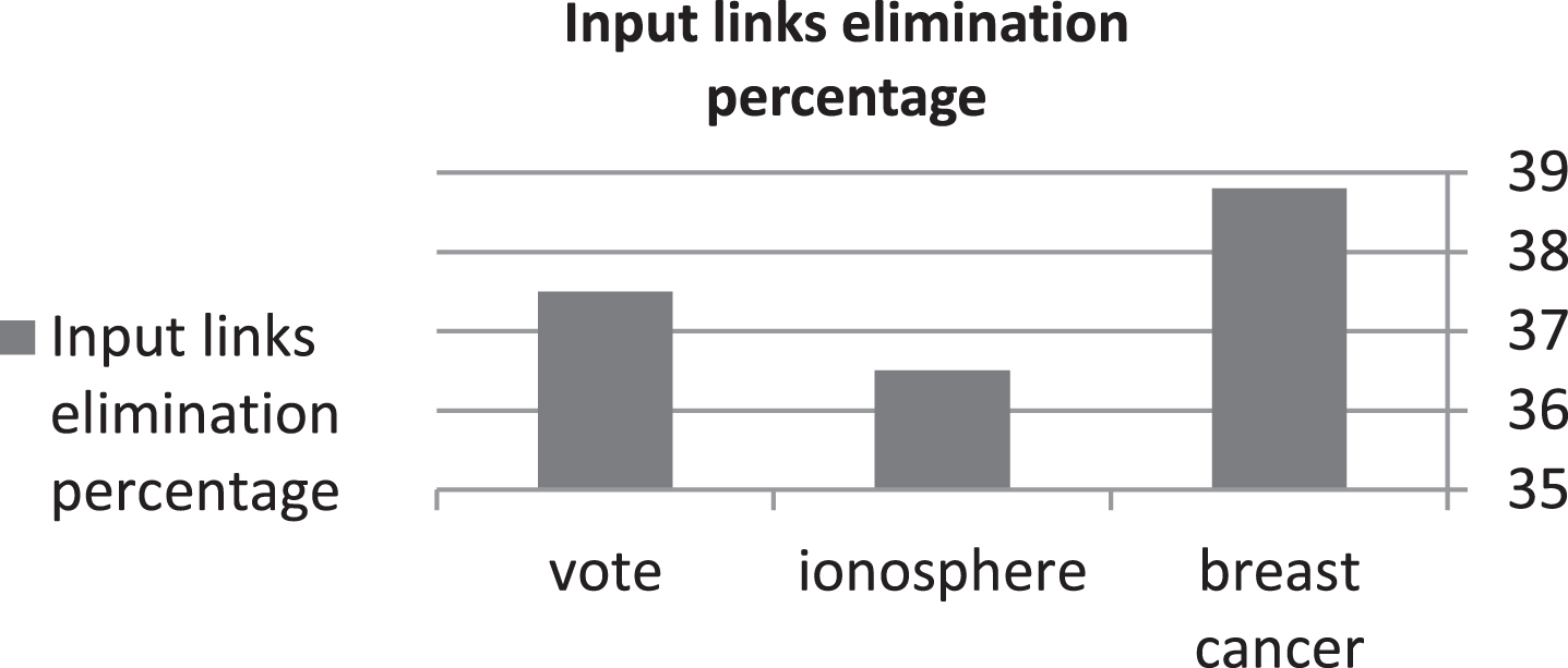
The elimination percentage in the input links from all the input connections in the ANN.

Table 5

The remaining input links after applying NNPII

dataset	Original input links	Input Links after applying NNPII
breast cancer	18	11
ionosphere	238	151
vote	32	20

It is noticed from the obtained figures and tables that the elimination percentage is depending on the number of instances, the more is the number of instances, the more is the percentage of input links elimination, but this might not be always true.

5.3 NNPII with various parameters values

In this experiment we apply NNPII on iris dataset with various parameter values concerned directly with the proposed algorithm. iris dataset has 150 instances with 5 attributes including the class. All the attribute values are real values except the class attribute which has three possible valuesIris-setosa,Iris-versicolor,Iris-virginica. We fix δ as 0.2 and keep changing the values of number of partitions p_i for real datasets and number of randomly selected instances m. Table 6 shows the obtained results when m is fixed as 40% of the total number of instances and varied number of partitions. Table 7 shows the results accuracy of iris datasets with various m and p_i values.

Table 6
Iris classification accuracy using fixed m and various p_i

Percentage of randomly instance selection # of partitions Results accuracy

40% 6 100%

7 93.1%

5 94.5%

9 94.5%

Percentage of randomly instance selection	# of partitions	Results accuracy
40%	6	100%
	7	93.1%
	5	94.5%
	9	94.5%

Table 7

Various results accuracy of iris datasets

Percentage of randomly instance selection	# of partitions	Results accuracy
30%	6	94.5%
50%	6	98.6%
60%	6	98.6%
70%	6	98.6%

From Table 6 and Table 7, we notice that the best obtained result is with 40% as percentage of randomly instance selection and 6 partitions. The results obtained using 50% as percentage of randomly selected instances and above with 6 partitions gave the same results (98.6%). This result could mean that the nature of the attribute values does not tolerate more partitions than 6 regardless of various values of p_i. Also 40% indicates that this much of randomly instance selection is enough to give better classification. However, even values above 40% are still giving good results. In our experiments we consider a fixed partition for all the attributes. It is to be noted that the number of partitions might differ from one attribute to another based on the nature of the data and that will definitely increase the results accuracy.

5.4 Comparison between NNPII and other pruning algorithms

In this section we perform a comparative study between NNPII results and the other results obtained by other pruning algorithms. Table 8 shows the datasets used for comparison.

Table 8
The datasets used for comparison between NNPII and other pruning algorithms

Dataset # of instance #of attributes including the class attribute Data type # of class values

breast cancer 699 10 real 2

iris 150 5 categorical 3

diabetes 768 20 integers 2

Dataset	# of instance	#of attributes including the class attribute	Data type	# of class values
breast cancer	699	10	real	2
iris	150	5	categorical	3
diabetes	768	20	integers	2

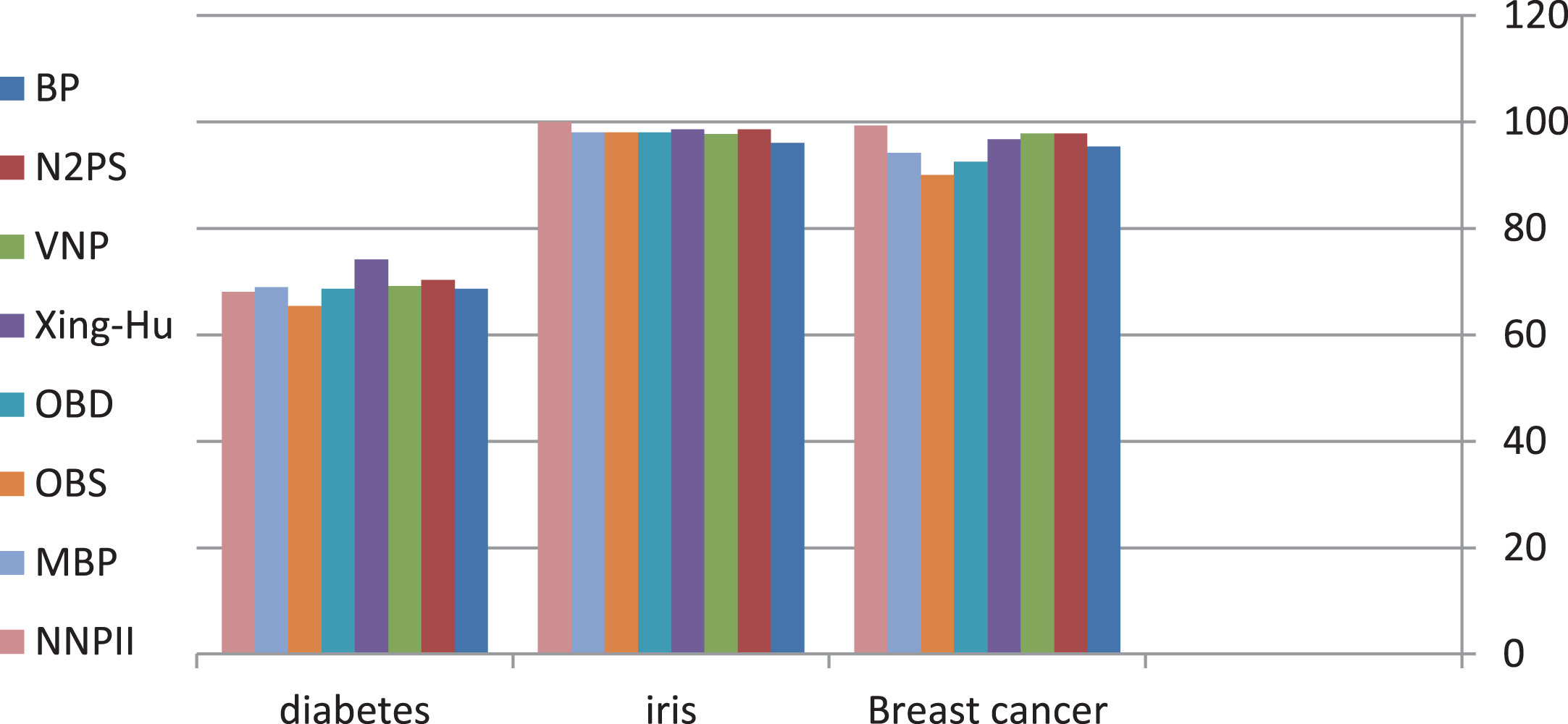
Table 9 and Fig. 3 show the results of the comparative study between NNPII algorithm and other pruning algorithms. The results presented here are related to BP,N2PS, VNP, Xing-Hu, OBD,OBS and MBP algorithms and have been taken from [4].

Fig.3

Comparative results between various pruning algorithms.

Table 9

Comparison of NNPII algorithm and other pruning algorithms

Dataset	BP	N2PS	VNP	Xing-Hu	OBD	OBS	MBP	NNPII
Breast cancer	95.4%	97.8%	97.8%	96.7%	92.5%	90%	94.2%	99.3%
iris	96%	98.6%	97.7%	98.6%	98%	98%	98%	100%
diabetes	68.6%	70.3%	69.1%	74.2%	68.6%	65.4%	68.9%	68.1%

Based on the obtained results, it is noticed that NNPII outperforms other pruning algorithms when breast cancer or iris datasets are used. In case of diabetes, NNPII does not perform well, but it still gives better performance than OBS. Xing-Hu approach outperforms all other approaches with diabetes dataset. The performance of NNPII using diabetes dataset is not bad comparing it with the other algorithms, the regression in the performance could be because the data instances are not distributed fairy among the class attribute values. The same reason could have the same effect on all the other algorithms. Because the NNPII algorithm depends on the nature of inputs, this leads to low accuracy. It is noticed that whenever there is a fair distribution in the dataset related to class attributes, NNPII performs better than other pruning algorithms. For example, in case of iris dataset, the class attributes are equally distributed where each class attribute has 50 instances, and in the case of diabetes 500 (65.1%) instances have value 0 and 268 (34.89%) have value 1, which indicates clearly that the class value distribution is unfair. In case of breast cancer, 458 (65.5%) have values benign and 241 (34.5%) malignant, which also indicates unfair distribution of class value attributes, but NNPII still gives the best results. One important issue to be considered is that the number of attributes in diabetes is 20, whereas the number of attributes in breast cancer is 10 with almost the same number of instances, this is one among other reasons that makes algorithms perform better with breast cancer comparing with diabetes as shown in Fig. 3. This is also valid for NNPII specially because the number of instances of diabetes dataset is small comparing to number of attributes with various possible values for each attribute (integers), this made it an obstacle for NNPII to decide correctly the importance of the data item. In the case of breast cancer, NNPII as other algorithms could perform well (even the best). This occurred despite that the data is not balanced, but NNPII could well recognize the importance of attributes because the data values for each attribute that can affect the results are clear within certain ranges in the dataset. To summarize, the reason why all the algorithms including the NNPII perform well using breast cancer is that there is a clear distinction in the value of attributes to classify benign or malignant whereas all the algorithms perform bad using the diabetes because the values of the given attributes are very close in a way classification becomes difficult and the number of instances is not enough to make the algorithms easily generalize. In brief, fair distribution of instances based on class attribute gives more opportunity to NNPII to perform better than other algorithms.

6 Conclusion

A pruning algorithm based on input importance called NNPII has been presented in this paper. NNPII is designed to remove only connections between the input layer and the hidden layer. NNPII has three stages, preprocessing stage, forward stage and backward stage. In NNPII, input importance is used to replace the real input. Pruning is performed throughout the training phase. Most of the previous works related to pruning, training and pruning are performed iteratively, which makes the training take a lot of time. Various experiments have been conducted. Results show the capability of NNPII to remove around 35% of the input connections. Comparing NNPII with various pruning algorithms, results show that whenever the class values are distributed fairly in the dataset, NNPII performs better than other algorithm, whereas when the distribution of the class values is not fair, NNPII still compete with other algorithms. The obtained results match with the logic of the NNPII algorithm, which depends on the nature of the inputs. Some future directions are considering pruning of nodes as well as the connections between the hidden layer and the output layer.

References

Abbasi-Asl and

Yu , Structural Compression of Convolutional Neural Networks Based on Greedy Filter Pruning, Cornell University arXiv:1705.07356v3 [cs.CV], 21 Jul 2017.

Abbasi-Asl and

Yu , Interpreting Convolutional Neural Networks Through Compression, Cornell University, arXiv:1711.02329v1 [stat.ML], presented at NIPS 2017 Symposium on Interpretable Machine Learning, 7 Nov 2017.

Augasta and

Kathirvalavakumar , A novel pruning algorithm for optimizing feedforward neural network of classification problems, Neural Processing Letters 34(3) (2011), 241–258.

Augasta and

Kathirvalavakumar , Pruning algorithms of neural networks - a comparative study, Central European Journal of Computer Science 3(3) (2013), 105–115.

Babaeizadeh ,

Smaragdis and

Campbell , NoiseOut: A SimpleWay to Prune Neural Networks, in the proceedings of the 29th Conference on Neural Information Processing Systems (NIPS), Barcelona, Spain, 2016.

Bondarenko ,

Borisov and

Aleksejeva , Neurons vs Weights Pruning in Artificial Neural Networks, Environment Technology, Resources III (2015), 22–28.

Castellano ,

Fanelli and

Pelillo , An iterative pruning algorithm for feedforwrd neural networks, IEEE Transactions on Neural Networks 8 (1997), 519–531.

Engelbrecht , A new pruning heuristic based on variance analysis of sensitivity information, IEEE Transactions on Neural Networks 12(6) (2001), 1386–1399.

Hagiwara , A simple and effective method for removal of hidden units and weights, Neurocomputing 6 (1994), 207–218.

10.

Han ,

Pool ,

Tran and

Dally , Learning both Weights and Connections for Efficient Neural Networks, Proceedings of Neural Information Processing System Conference, NIPS 2015, poster, 2015.

11.

Hassibi ,

D.G.

Stork and

G.J.

Wolf , Optimal brain surgeon and general network pruning, Proceedings of IEEE ICNN’93,1, WDS’08 Proceedings of Contributed Papers, Part I, (2008), 293–299.

12.

Lazarevic and

Obradovic , Effective Pruning of Neural Network Classifier Ensembles, Proceedings of International Joint Conference on Neural Networks, Washington, DC, USA 15–19 July 2001.

13.

Le Cun ,

J.S.

Denker and

S.A.

Solla , In.

D. S.

Touretzky (Ed.), Optimal brain damage, Advances in neural information processing systems (Morgan Kaufmann, San Mateo, 1990) 2 (1990), 598–605.

14.

Molchanov ,

Tyree ,

Karras ,

Aila and

Kautz , Pruning convolutional neural networks for resource efficient inference, 5th International Conference on Learning Representations (ICLR 2017), Toulon, France, April 24 - 26, 2017.

15.

Pan ,

Dong and

Guo , DropNeuron: Simplifying the Structure of Deep Neural Networks, Cornell University, arXiv, :1606.07326v3 [cs.CV] 3 Jul 2016.

16.

Ponnapallii ,

Ho and

Thomson , A formal selection and pruning algorithm for feedforward artificial neural network optimization, IEEE Transactions on Neural Networks 10(4) (1999), 964–968.

17.

Sabo and

Yu , A new pruning algorithm for neural network dimension analysis, International Joint Conference on Neural Networks (2008), 3313–3318.

18.

Schiavo , Two methods for pruning neural networks: A performance evaluation, Statistica Applicata 13(1) (2001), 75–88.

19.

Stepniewski and

Keane , Pruning backpropagation neural networks using modern stochastic optimization techniques, Neural Computing and Applications 5(2) (1997), 76–98.

20.

Suzuki ,

Horiba and

Sugie , A Simple Neural Network Pruning Algorithm with Application to Filter Synthesis, Neural Processing Letters 13 (2001), 43–53.

21.

UCI Machine Learning repository, https://archive.ics.uci.edu/ml/datasets.html

22.

H.-J.

Xing and

B.-G.

Hu , Two phase construction of multilayer perceptrons using Information Theory, IEEE Transactions on Neural Network 20(4) (2009), 715–721.

23.

Yilmaz , Artificial neural networks pruning approach for geodetic velocity field determination, BCG - Boletim de Ciências Geodésicas 19(4) (2013), 558–573.