
Abstract
Horizontal cooperation in logistics refers to several logistics service providers cooperating to accomplish common goals, which usually involves a collaborative vehicle routing problem. In this paper, we present a new collaborative vehicle routing problem with rough location (CVRPRL), which considers both the security of sharing detailed customer information and the configuration of shared resource. We utilize the rough location of the customer to replace the detailed customer location and introduce the concept of collaborative logistics sharing degree in the CVRPRL model. Subsequently, the cost allocation mechanism is designed based on an extended Shapley value, which allocates fixed costs and risks in different ways. Further, an extended ant colony optimization (EACO) algorithm is proposed to solve the CVRPRL. The EACO algorithm combines both large neighborhood search and local search strategies. Finally, we perform a series of simulation experiments to verify the effectiveness of EACO compared with other meta-heuristic algorithms.
Keywords
Introduction
In recent years, fierce competition in global markets, increasing transportation cost, the introduction of products with shorter life cycles, and the heightened expectations of customers have created enormous pressure on logistics service providers (LSPs) [8]. To address this challenge, LSPs are increasingly cooperating with each other. If cooperation occurs at the same level of the supply chain, it can be called horizontal cooperation [26] and these LSPs form horizontal logistics coalitions. Since horizontal cooperation was introduced, many researchers have devoted time and effort to collaborative vehicle routing problem (CVRP) [5, 11, 14, 16, 18], whose objective is to have several LSPs cooperating with each other to accomplish transportation tasks with minimum cost routing.
Most existing studies on the CVRP consider resource sharing separate from partners’ strategies and cost allocation, though the former usually affects the latter to a certain extent. First, sharing customer information with partners, who are often previous competitors, may be unacceptable to decision makers. However, in previous studies on the CVRP, the detailed customer location was usually made public in a routing plan. Second, resource sharing may affect the strategies of LSPs. However, previous studies on the CVRP assumed that the horizontal logistics coalition could control all the resources of each LSP to optimize the overall logistics distribution network. In this situation, the long-term strategy of LSPs will be affected because most of their resources are utilized by the horizontal logistics coalition. Third, cost allocation involves the risk cost of each LSP, which is related to the amount of resource sharing.
The aim of this study is to propose a novel CVRP with rough location (CVRPRL) that integrates both resource sharing and partners’ strategies, and then present a novel cost allocation mechanism that involves risk factors. In the proposed CVRPRL model, LSPs can only offer a rough location (RL) of the customer to hide sensitive business information in the negotiation stage. For example, LSPs only offer the location of an industrial district, instead of a detailed factory location. To reduce the impact of the uncertainty caused by RL on the actual situation, a fuzzy delivery time based on the credibility theory is applied to this problem. Moreover, each LSP can adjust its own shared resource configuration to maintain balance between itself and the coalition. In this study, the concept of collaborative logistics sharing degree (CLSD), which represents the configuration of the shared resources of LSPs is introduced in the CVRPRL. Finally, the cost allocation mechanism is designed based on the extended Shapley value, which allocates fixed costs and risks in different ways.
As an extension of the vehicle routing problem (VRP), the CVRPRL addressed herein is more complex because it considers more factors. In previous studies, the ant colony optimization (ACO) [12] algorithm has been employed to effectively address various VRPs [15, 19, 23]. The standard ACO algorithm is modeled on the ants’ group behavior, which has positive characteristics like positive feedback and self-organization. However, the standard ACO algorithm tends to trap in local optimum and its convergence rate is slow. Thus, in order to address CVRPRL better, we propose an extended ant colony optimization (EACO) algorithm. In this study, we mainly extend the standard ACO algorithm to address intrinsic shortcomings from three aspects. First, a modified solution construction mechanism is applied to accelerate the convergence speed. Then the EACO algorithm is integrated with a large neighborhood search (LNS) [30] algorithm to improve the optimization performance. Finally, some local search strategies are integrated to improve the global search ability of the algorithm. To verify the effectiveness and feasibility of the EACO algorithm, a series of simulation experiments were conducted as described in Section 5 to compare the proposed algorithm with other meta-heuristic algorithms.
The rest of this paper is organized as follows. In Section 2, the relevant works are discussed. In Section 3, a description of CVRPRL model and the extended Shapley value are provided. In Section 4, the basic ACO algorithm is introduced and the EACO algorithm is proposed. In Section 5, experiments are conducted to verify the effectiveness and feasibility of the EACO algorithm. Finally, Section 6 summarizes the study and provides suggestions for future research.
Related work
Collaborative vehicle routing problem
The VRP was proposed by Dantzig and Ramser [10]. The conventional VRP is to find a set of routes incurring minimum operational cost to serve a set of customers [2]. During the past decade, VRP and its extended class have been a research hotspot, e.g., dynamic VRP [28], pickups and deliveries problem with fuzzy time windows [6] and capacitated VRP with two-dimensional loading constraints [33].
To increase competitive advantage, logistics companies begin to establish collaborative relationships. Thus, CVRP has been recently paid more attention from researchers. Dai and Chen [9] studied collaborative logistics and proposed three profit allocation mechanisms based on the Shapley value model. Kimms and Kozeletskyi [17] studied cost allocation based on the Shapley value in cooperative traveling salesman problem under rolling horizon planning. In a study of Wang et al. [31], collaborative multiple-center vehicle routing is optimized by adjusting vehicle routes among multiple distribution centers. An improved Shapley value model with optimal sequential selection is proposed to distribute the gained profits among LSPs. To further improve the benefit, Defryn et al. [11] studied a selective vehicle routing problem in a collaborative environment where strategic behavior of each partner is defined by the compensation for non-delivery. To optimize logistics network, Wang et al. [32] developed a bi-objective model for optimizing collaborative two-echelon network. Fernàndez et al. [14] presented a shared customer collaboration VRP for horizontal collaboration in the framework of last-mile deliveries. By sharing customer orders, LSPs can obtain a collaborative scheme which makes them more competitive.
In summary, the above studies showed that collaborative vehicle routes can improve the efficiency of LSPs, and proposed various cost allocation schemes. However, previous studies on CVRP assume that all shared resources of each LSP can be controlled by coalition in which the partners’ strategies or decisions are ignored. In addition, the literature that discusses the risk factors in CVRP is lacking. Thus, this study aims to propose a more practical model to address these problems. On the one hand, the CVRPRL model can ensure LSP managing its own shared resources and guarantee their information security. On the other hand, the risks are considered in cost allocation.
Ant colony optimization algorithm
The ACO algorithm was first proposed by Dorigo [12]. It was inspired by the behavior of an ant seeking the shortest path to a food source. However, the ACO also has some shortcomings including the slow convergence rate and stagnation. Thus, many researchers developed various extensions of ACO algorithm to address above shortcomings. Yu and Yang [35] proposed an improved ACO algorithm to address a period VRP with a time window. The improved ACO algorithm contains a multi-dimension pheromone matrix to accumulate heuristic information on different days and uses two-crossover operations to improve its performance. In addition, some researchers applied local search strategies to further improve the performance of ACO algorithm. Li et al. [19] addressed an open VRP through a hybrid ACO algorithm that integrated a tabu search and applied local search techniques. Yousefikhoshbakht et al. [34] combined several effective local search techniques with the ACO algorithm to solve an open VRP.
Recently, several researchers begin to study how to integrate ACO algorithm with other meta-heuristic algorithms to address VRP efficiently. Elhassania et al. [13] hybridized the LNS algorithm with the ACO algorithm for solving dynamic VRP. The experimental results show that the new hybrid ACO algorithm can obtain satisfactory solutions for dynamic VRP. Brito et al. [4] applied a hybrid meta-heuristic algorithm to address a close-open VRP with time windows. In the hybrid meta-heuristic algorithm, greedy randomized adaptive search algorithm generates new solutions based on heuristic information from ACO algorithm and the VNS algorithm is applied to improve the solution. To solve the capacitated VRP, Akpinar [1] hybridized the LNS algorithm with the ACO algorithm, in which, the solution construction mechanism of ACO algorithm is embedded into the LNS to improve the solution.
As mentioned before, various extensions of ACO have been proposed to address VRP. However, few studies have explored the use of an ACO algorithm in solving the CVRP. In fact, because above studies only consider single depot or single LSP, most of them cannot deal with CVRP directly. Thus, we propose an EACO algorithm for solving the CVRPRL in this work. Inspired from previous studies, EACO algorithm is integrated with LNS algorithm to avoid the shortcoming of basic ACO algorithm. Therefore, we propose a heuristic removal operation and the application of a local search strategy to further improve the performance of the EACO algorithm.
Collaborative vehicle routing problem with rough location
Model formulation
In this section, we describe the CVRPRL model. We consider a set of customers C, a set of depots D, and a fixed fleet of homogeneous vehicles K. Traditional CVRP aims to find an optimal routing plan with minimum transportation cost in disregard of the partner’s strategy. Instead, the proposed CVRPRL model integrates both resource sharing and partner’s strategy. The notations to be defined in this model are given as follows:
Notations
(1) Sets:
set of depots
set of customers
set of customers who belong to LSP l
set of nodes, N = C ∪ D
set of vehicles
set of LSPs
(2) Input variables:
the delivery cost between RL i and RL j
the delivery cost from customer i to customer j, servedby its own LSP
the delivery cost in RL i
the RL area of node i (Note that the RL area of depot equals 0 because it is not necessary to hide the detailed depot location)
the RL girth of node i (Note that the RL girth of depot equals 0 because it is not necessary to hide the detailed depot location)
the fuzzy delivery time between node i and node j
the due time of customer i
the capacity of products needed by customer i
the vehicle capacity ∂ the confidence level
the maximum of shared freight capacity of LSP l
the maximum of shared warehouse inventory of LSP l
the maximum number of shared customer orders of LSP l
the maximum sharing degree of LSP l
(3) Decision variables:
x ijkl = 1 if the vehicle k of LSP l transports from node i to node j (i, j ∈ N, k ∈ K, l ∈ L); otherwise set x ijkl = 0
the fuzzy arrival time at node i
Rough location
In traditional studies of the CVRP, the customer’s detailed location is visible to all LSPs, which will compromise the security of customer information. In the proposed CVRPRL, LSPs will offer RLs to their partners to protect sensitive information. Figure 1 shows illustrative examples of a non-cooperative routing plan, traditional cooperative routing plan, and cooperative routing plan with an RL. From Fig. 1(a) and 1(b), we can see that both LSP A and LSP B can optimize their respective routes through cooperation, but they have to reveal their respective customer’s detailed location to each other. As shown in Fig. 1(c), both LSP A and LSP B can only obtain the RL of the other’s customer but can still optimize the collaborative routing plan. If a customer order is outsourced to another LSP, the travel cost depends on the distance between the RLs and their areas. It is noted that the area of an RL will affect the entire logistics activity. The larger the area of the RL, the more uncertain the collaborative route is. Thus, if the area of the RL is too large, it will increase the overall operational cost. If the area of the RL is too small, the security of customer information cannot be guaranteed. In this study, if a LSP’s customer is served by other LSPs, the LSP will incur an extra penalty cost that is determined by the area and girth of the RL. The configuration of an RL depends on the LSP’s strategy.
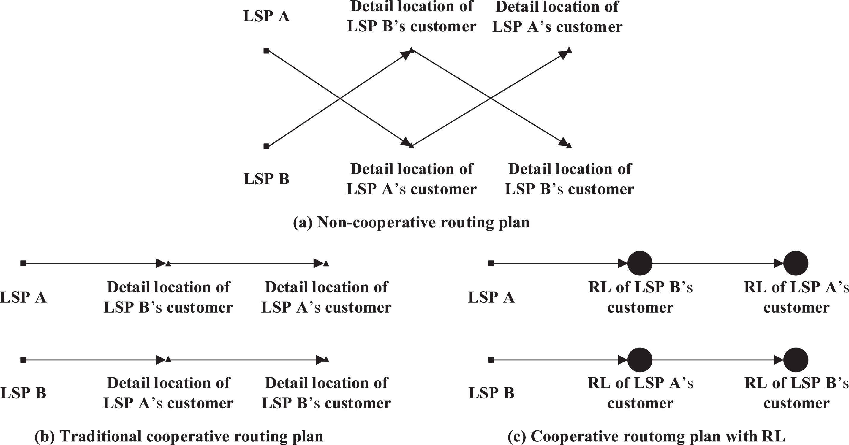
Illustrative examples of different routing plans.
In traditional studies on CVRPs, all the shared resources of LSPs are controlled by a horizontal logistics coalition. In the proposed CVRPRL, LSPs can adjust their respective shared resources according to the CLSD from three aspects: freight capacity sharing degree (FCSD), warehouse inventory sharing degree (WISD), and customer order sharing degree (COSD). First, an LSP usually does not share all freight capacity in the horizontal logistics coalition so that it can use its remaining freight capacity in its own future expected plans. In this study, the shared freight capacity can be expressed as the transportation cost from the other LSPs’ customers and Equation (1) shows the FCSD of LSP l. Second, an LSP usually does not share all warehouse inventory in the horizontal logistics coalition so that it can use the remaining inventory for its own future customer orders. In this study, the shared warehouse inventory can be expressed as the total capacity of products that is used to meet the other LSPs’customers and Equation (2) shows the WISD of LSP l. Third, an LSP usually does not share all customer orders in the horizontal logistics coalition so that it can fulfil the remaining customer orders itself. In this study, the shared customer order can be expressed as the number of outsourced customer orders and Equation (3) shows the COSD of LSP l. Equation (4) shows that the CLSD of LSP l consists of FCSD, WISD, and COSD.
In addition, the larger the RL area of the outsourced customer, the more unreliable the overall routing is. In Equation (1), besides the consideration of explicit transportation costs
The objective function is to minimize the overall operational cost, consisting of two parts. The first part is composed of the transportation costs to arrive at RL and the delivery cost in RL, which involves a penalty mechanism to limit the area size of RL. The second part is the delivery cost of customerservedby its own LSP. Thus, the objective function of the CVRPRL model is defined as follows:
Subject to the following constraints:
Equation (6) shows that each customer is visited exactly once. Equation (7) represents that the amount of outgoing vehicles is equal to the amount of incoming vehicles at each node. Equation (8) shows that the CLSD of LSP l is no more than its MCLSD, which avoids the LSP l from sharing excessive resource. Equation (9) represents the fuzzy arrival time at customer j from depot i. Equation (10) represents the fuzzy arrival time at node j from customer i. Equation (11) shows that each vehicle is not overloaded.
In this model, the arrival time is presented by trapezoidal fuzzy number ℓ = (ℓ 1, ℓ 2, ℓ 3, ℓ 4). In order to rank them, we employ credibility measure [20] in CVRPRL model. According to the nature of this problem, coalition should provide a confidence level ∂ where the decision must meet the constraints at the defined confidence level. According to the credibility theory, we can derive the credibility with which the vehicle arrives at the customer before due time.
Equation (13) shows that the credibility with which the vehicle arrives at the node within the due time equals or exceeds the confident level.
It can be found that the cost of optimal solution from CVRPRL will be possibly higher than that from the traditional CVRP model. There are two main reasons. On the one hand, there exist more uncertain factors in the proposed model due to RL. On the other hand, the resource distribution and management encounters more constraints from LSP. These issues need be addressed in the future work so that the logistics network based on CVRPRL becomes more stable and brings more potential benefits.
The time complexity of calculating the CVRPRL model can be divided into three parts. First, the CLSD of all LSPs are obtained by enumerating each customer, which requires O (|C|) time. Second, the fuzzy arrival time of all customers is obtained by enumerating each route, which requires O (|C| + |D| * |K|) time. Third, the overall travelling cost is obtained by adding up the costs of all routes, which requires O (|C| + |D| * |K|) time. |D| * |K| is equal to the total number of vehicles, which is much lower than the number of customers in a real-world situation. Thus, the time complexity of calculating the CVRPRL model is O (3 * |C| + 2 * |D| * |K|), which is approximately equal to O (3 * |C|). Therefore, similar to the time complexity of calculating the traditional CVRP model, the time complexity of calculating the CVRPRL model will increase linearly with the number of customers.
Shapley value
Allocation strategy is critical in cooperative logistics [21]. The Shapley value is proposed by Shapley [29] for profit or cost allocation. Let us define the set N of LSPs, the power set of P (N), and the payoff function v. Each subset of N is called a coalition, excluding null set. The following two conditions should be satisfied:
Equation (14) shows that void coalition has no cost value. Equation (15) shows that the cost value of two mutually cooperative coalitions is less than or equal to that of two independent coalitions; two mutually cooperative coalitions can incur less cost. In the coalition S, the marginal cost φ of LSP i is calculated by Equation (16).
ζ (S, v) represents the Shapley value of coalition S, and is calculated by Equation (17).
The allocation cost of a LSP is the weighted sum of marginal costs in the coalition. However, in the process of cooperation, emergency issues such as vehicle damage or cargo loss may impact the actual cost. The risk of logistics coalition should also be considered in the allocating strategy. Next, we will extend Shapley value by including the risk of logistics to solve this problem.
In this study, the overall cost consists of fixed cost and risk cost. Based on the extra cost of risk and the amount of resource sharing of each LSP, we propose an extended Shapley value. By comparing with the fixed cost, the allocation scheme for risk cost will be adjusted. The payoff function v is composed of fixed payoff p
f
and risk payoff p
r
. p
f
(S) represents the minimum fixed fuel cost of coalition S, which is given by the CVRPRL model. p
r
(S) represents the additional cost of coalition S based on risk assessment. The payoff function v and modified marginal cost φ
e
are calculated as follows:
Basic ACO algorithm
Based on the way an ant seeks food sources, the ACO algorithm was first proposed by Dorigo [12] to determine the best path in a graph. ACO algorithm has been widely applied to the vehicle routing problem. Initially, the ant will randomly select the next customer until each customer has been visited. Ants will leave their pheromone in the trail. Subsequently, in each iteration, the ant will select the next customer using a heuristic search. The probability of selecting node j when ant k is at node i is described as follows:
After each ant finds the solution in an iteration, the pheromone of the trail will be updated. Equations (23 and 24) show the updated mechanism.
ρ is a parameter representing the evaporation rate and L k is the total distance that the ant k travels.
The ACO algorithm has advantages such as positive feedback, self-organization, and heuristic search ability, which render it applicable to various VRPs. However, as the number of customers increases, the standard ACO algorithm is ineffective to solve this class of problem. The main reason is that the ACO algorithm lacks powerful local search ability and tends to stagnate in the local optimal solution. To overcome these issues, the EACO algorithm is proposed. In each iteration, we apply a modified construction mechanism to initialize a colony. Subsequently, a heuristic removal operation is employed to adjust the current best solution and the global best solution. Further, the nodes with minimum cost are re-inserted and local search strategies are applied to further improve the solution. The main procedure is shown in Fig. 2.

Main procedure of EACO.
In the ACO phase, the ants will construct solutions according to heuristic information. It can be considered as an optimized heuristic clustering process and a better solution can be found. In traditional studies of ACO, the solution construction process largely depends on the pheromone, which tends to lead to stagnation. Therefore, we improve the construction mechanism in the current study by employing three rules randomly to avoid stagnation. A new route between node i and node j can be built based on Equation (25).
After the construction phase, we use the local search to optimize the current best solution and the global best solution. The LNS algorithm applies removal operation and re-insertion operation to the initial feasible solutions to improve the solution. Ropke and Pisinger [27] proposed the worst removal heuristic to replace Shaw removal heuristic [30]. In the worst removal heuristic, the higher the transportation cost a customer incurs, the likelier it is that the customer is removed. However, some customers may be removed by mistake if they are too far away from other customers. Figure 3 shows an illustrative example by using conventional worst removal heuristic to remove customer, in which, two customers A and B, who are far away from other customers, will be removed by mistake with high probability.
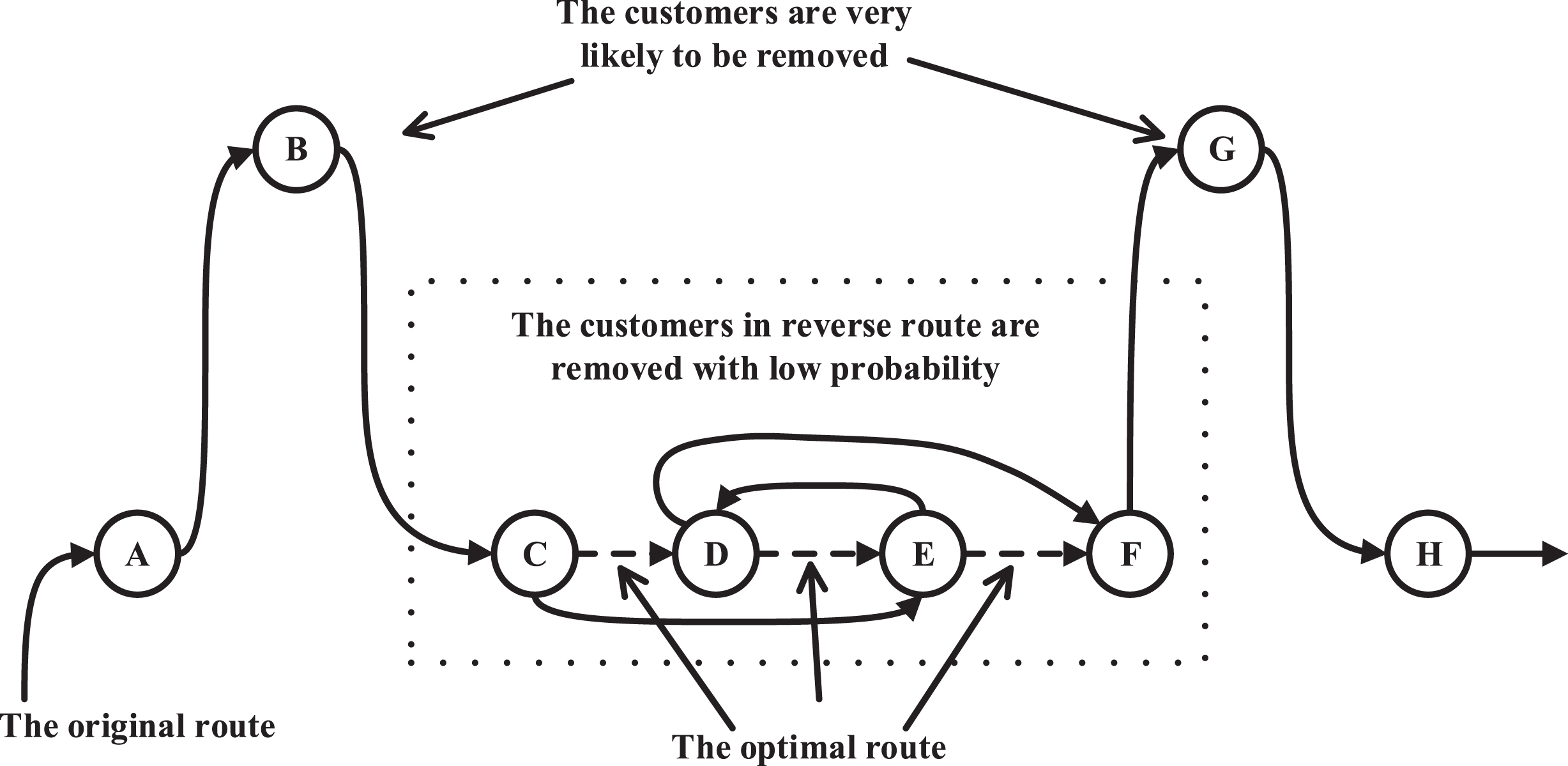
Using conventional worst removal heuristic to remove customers.
In this work, a modified worst removal heuristic is proposed, according to which, a customer that incurs abnormally high transportation cost should have higher probability of removal. In Fig. 3, two customers A and B, who are very likely to be removed by conventional worst removal heuristic, are served with normal transportation cost and are less likely to be removed by our modified worst removal heuristic. Four customers C, D, E and F, who are less likely to be removed by conventional worst removal heuristic, are served with abnormally high transportation cost due to reverse route and can be very likely to be removed by our modified worst removal heuristic. The abnormal cost (AC) and the corresponding probability are calculated by Equations (26) and (27) respectively.
Although a basic ACO can be used to find a solution for a VRP, the basic ACO tends to be the stagnation after a certain time of iteration. The drawback can be avoided by combining other approaches. In some studies [19, 34], the local search strategy is often applied to further improve the performance of ACO. In the current study, we also apply the local search strategy to further improve the optimization performance of EACO, which consists of a 2-opt algorithm [7] and an Or-opt algorithm [25]. The 2-opt algorithm is an effective local search technique that reverses a segment of a route to obtain a better solution, unless the solution cannot be improved further. As an illustrative example, Fig. 4(a) shows that the segment of the route from node B to node D is reversed. Similarly, the Or-opt algorithm is used to reverse a segment of a route, and then change the position of the segment in the route to obtain a better solution, unless the solution cannot be improved further. As another illustrative example, Fig. 4(b) shows that the segment of the route from node A to node B is reversed first, and is then inserted between node D and node E.

The operations of 2-opt and Or-opt.
The local search strategy offsets the mistakes made by the greedy re-insertion operation, which sometimes inserts a costly route. The pseudo code of the 2-opt and Or-opt algorithms are shown in Algorithm 2 and Algorithm 3, respectively.
To analyze the proposed model, we use an illustrative example to compare the performances of the cooperative and non-cooperative modes. To test the performance of the EACO algorithm, a series of simulation experiments were conducted. First, we test the performance of the EACO algorithm by some already solved instances. Second, we test the performance of the EACO algorithm by comparing it with the ACO [3], LNS, and ACOLNS [13] algorithms. The ACOLNS algorithm is a hybrid of ACO and LNS. The LNS algorithm uses the Shaw removal heuristic [30] and greedy reinsertion. Third, we test the performance of the EACO algorithm by comparing it with two other non-ACO inspired meta-heuristics algorithms, i.e., the variable neighborhood search (VNS) algorithm [24] and iterated local search (ILS) algorithm [22] that have been employed to successfully address the travelling salesman problem. The ILS and VNS algorithms both have an operation called perturbation or the shaking operation that randomly changes the current solution so that it does not get stuck at the local optimum. However, the shaking operation of an ILS algorithm [22] cannot be directly used in our model because it only considers a single depot and a single vehicle. In this experiment, the shaking operation, which is proposed by Meng et al. [24], is integrated in the ILS algorithm to address this issue. All the algorithms are coded in Java and run on a computer with Intel Core(TM) i5-7300HQ 2.50 GHz and 8 GB RAM operating on Microsoft Windows 10 operation system.
Experimental design
Owing to the lack of benchmarks involving RL and CLSD in the vehicle routing topic, we generate the data consistent with the real-world case via computer simulation. The ranges of MCLSD and confidence level are set to [0.50, 0.95] and [0.80, 0.95], respectively. Based on the size and location of RL, the fuzzy delivery time and transportation cost are generated randomly within a certain range. All experimental data have been public in the Figshare database (https://doi.org/10.6084/m9.figshare.6194165). In this experiment, LSPs use a circular region as RL and different RLs can have different sizes.
The parameter setting is presented in Table 1. α, β, and ρ represent the importance of pheromone, distance, and evaporation rate, respectively. R represents the fixed number of customers removed in ACOLNS. n ts and T control the number of removal and re-insertion operations in each iteration of ACOLNS, respectively. Δ controls the number of customers removed in the removal operations of LNS, ACOLNS, and EACO. r1, r2, q0, and p are user parameters. The η controls the node removal probability in the removal operations of VNS. The parameter settings of ACO, LNS, ACOLNS and VNS algorithms are obtained from Bell and McMullen [3], Shaw [30], Elhassania et al. [13] and Meng et al. [24], respectively. The population and number of iterations of all algorithms are set as 10 and 200, respectively.
Parameter setting
Parameter setting
In this section, we focus on the CVRPRL model. Table 2 shows the information of LSPs A, B, and C, which have 28 customers, 19 customers, and 30 customers, respectively. Figure 5 shows the simulated routing in both cooperative mode and non-cooperative mode. The square, star, and circle indicate the detailed location of customer, depot, and RL, respectively.
Small instance of collaborative vehicle routing problem
Small instance of collaborative vehicle routing problem
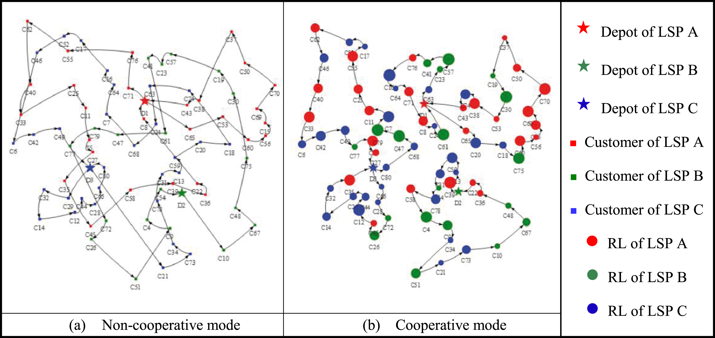
Routing in cooperative mode and non-cooperative mode.
Table 3 and Fig. 5(a) show the feasible routing plans of LSPs A, B and C under the non-cooperative mode. Some customers are far away from depots of their own LSPs, but are close to depots of other LSPs. Overlapping which appears among routes of different LSPs cause huge transportation cost.
Feasible routes under non-cooperative mode
After forming horizontal logistics coalition, Table 4 and Fig. 5(b) show the optimal logistics network. Most of customers are clustered around their neighbor depots. From Table 4, we can observe the cost of each coalition, which can be calculated using EACO algorithm.
Feasible routes based on cooperative mode
Table 5 also shows the result of cost allocation in the coalition. We can observe the expected additional risk cost of each coalition, which is usually calculated using risk assessment. According to Table 5, the cooperative mode can yield benefits for all LSPs. The greater the scale of the coalition, the lesser is the cost incurred. Compared with the conventional Shapley value, the proposed extended Shapley value considers extra cost caused by some risks to ensure the stability of the horizontal logistics coalition. Based on the extended Shapley value, LSPs A, B, and C will experience a cost reduction of 44.7%, 43.6%, and 26.4%, respectively, if they form a horizontal logistics coalition.
Cost distribution based on extended Shapley value
To analyze the impact of CLSD on the entire logistics process, the sensitivity of MCLSD is analyzed. The experiment shows the change in MCLSD with respect to the overall operational cost. The MCLSD of each LSP is the same and the example involves 3 LSPs, 97 customers, and 9 vehicles. Figure 6 shows the experimental result indicating that the overall operational cost gradually decreases with the increase in MCLSD. The amount of resources sharing in the coalition determines the logistics network.
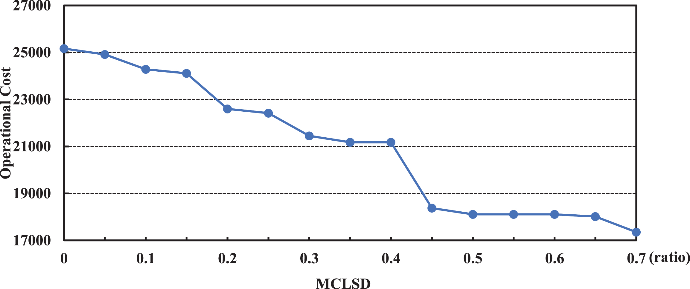
Overall operational cost with different MCLSDs.
In this sub-section, we focus on validating the optimization performance of EACO. Three problem sets with different configurations are illustrated. Table 6 lists the randomly generated values of problem set A. The number of depots ranges from 2 to 3. The number of customers ranges from 8 to 10. The total number of vehicles ranges from 2 to 4. The optimal solutions of problem set A are found by exhaustive computer enumeration. Table 7 lists the randomly generated values of problem set B. The number of depots ranges from 2 to 3. The number of customers ranges from 20 to 50. The total number of vehicles ranges from 2 to 9. Table 8 lists the randomly generated values of problem set C. The number of depots ranges from 2 to 4. The number of customers ranges from 35 to 55. The total number of vehicles ranges from 2 to 8. For each instance, the best cost, worst cost, average cost, and average running time are obtained by running the corresponding algorithms 10 times independently.
Used data in problem set A
Used data in problem set A
Used data in problem set B
Used data in problem set C
First, we analyze the performance of six algorithms by setting different population sizes and iteration numbers. Figure 7 shows the evolutionary trajectories of the six algorithms for instance DATA_N_35_D_2_V_2. From Fig. 7, the six algorithms all converge through 200 iterations. Figure 7 shows that the local search strategies can enhance the EACO algorithm to find a better solution.
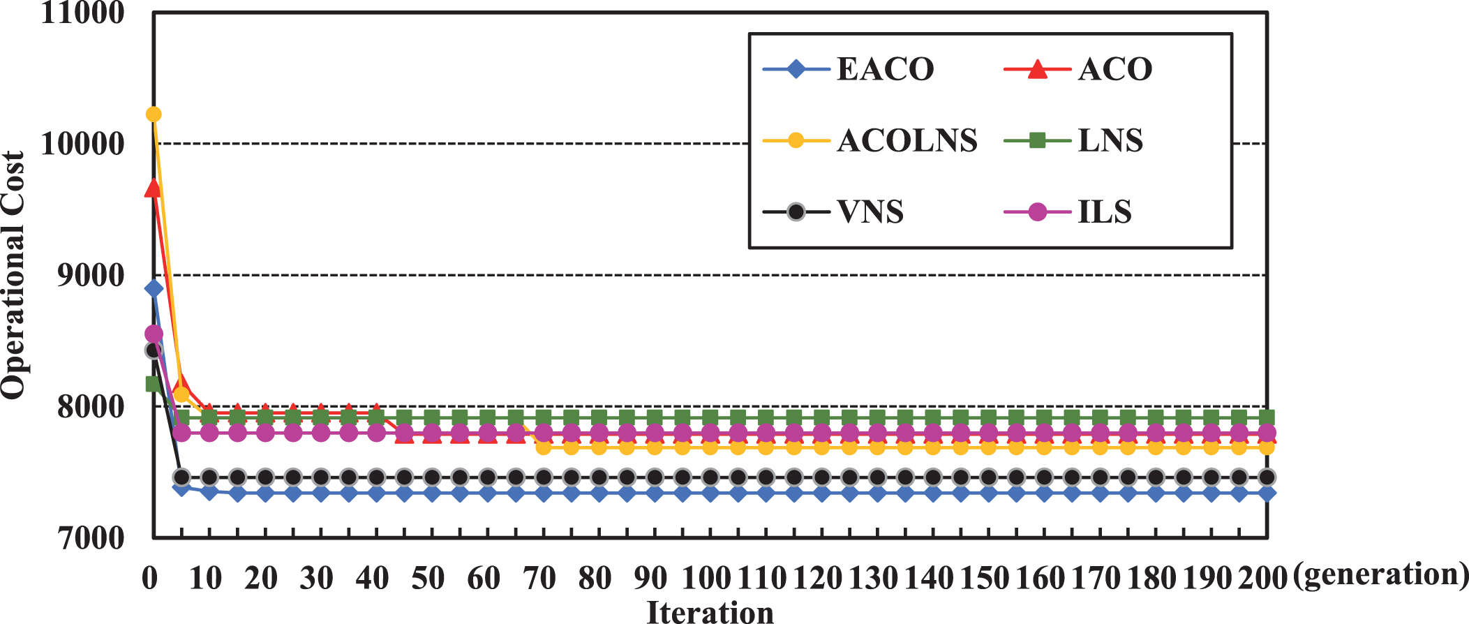
Evolutionary trajectories of the six algorithms.
Figure 8 shows the performance of the six algorithms in different population sizes for the instance DATA_N_35_D_2_V_2. As the population sizes increase, the VNS algorithm becomes slightly unstable, and the other algorithm is stable when population sizes are over 10. It can be found from Fig. 8 that the performance of EACO is stable with different population sizes. There are two main reasons. First, in the EACO algorithm, the LNS algorithm can further improve the algorithmic performance by avoiding the worst solutions. Second, local search strategies can improve the strong local search ability of EACO algorithm. Thus, although the population size changes, the EACO algorithm can still obtain high quality solutions in most situations and it is more stable than other algorithms.
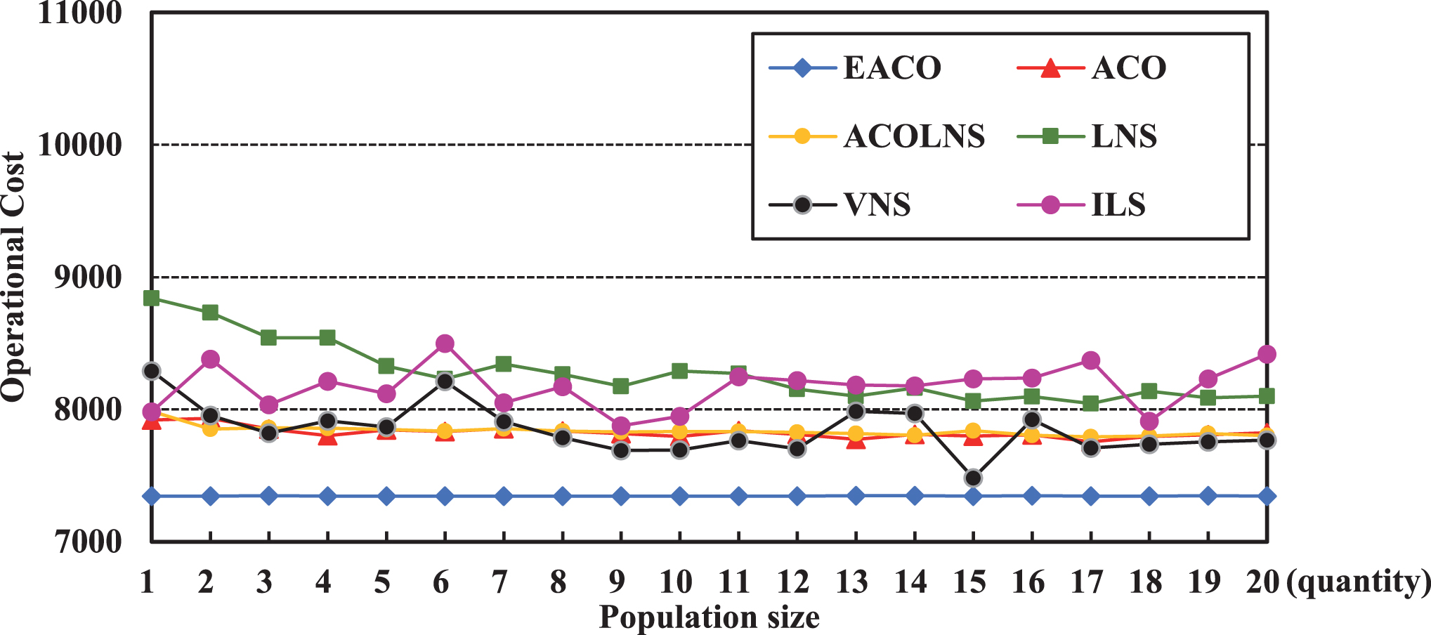
Performance of the six algorithms in different population sizes.
Table 9 shows the results after the EACO algorithm addresses problem set A. We can show that the EACO algorithm can find optimal solution for all instances in a short time.
Statistical results of EACO addressing problem set A
Table 10 presents the result of a comparison between the proposed EACO algorithm and three other baseline algorithms, which are the ACO, ACOLNS, and LNS algorithms. The EACO algorithm always finds the best solution. Notably, the runtime of the EACO algorithm is longer than those of the other algorithms, owing to its use of a local search to eliminate the local optimum. From Table 10, we can also observe that the runtime increases with an increase in the number of vehicles and the number of customers. However, the total runtime in this study is within the acceptable range. Presently, the costs of computer hardware resources have been reduced to some extent, and with the development of cloud computing, the runtime in this study will be reduced exponentially.
Statistical results of four algorithms addressing problem set B
Table 11 presents the result of a comparison between the proposed EACO algorithm and two non-ACO inspired meta-heuristics algorithms, i.e., the VNS and ILS algorithms. Although the VNS and ILS algorithms can address the problem in a short time, the EACO algorithm can find a better solution. In addition, the difference between the best cost and worst cost for the EACO algorithm is the smallest, indicating that its stability outperforms that of the VNS and ILS algorithms.
Statistical results of three algorithms addressing problem set C
In summary, LSPs can experience greater cost reduction by optimizing the logistics network. The CLSD of LSPs will impact the collaborative distribution network. Therefore, the proposed EACO algorithm can find a better solution than the other five heuristic algorithms.
Owing to the increasingly fierce market competition, more LSPs have begun to participate in horizontal logistics coalitions and they are focusing on the CVRP. However, LSPs will refuse cooperation in the case of unreliable partners, risk in the cooperation process, and lack of a fair distribution mechanism. In this paper, we proposed the CVRPRL model and an extended Shapley value to improve the feasibility of horizontal logistics coalition. Subsequently, EACO algorithm was proposed for solving the CVRPRL model, which combines both LNS and local search strategies. According to the experimental results, LSPs could achieve substantial gain under the novel cooperative mode. In addition, the EACO algorithm could find a better solution than the other five heuristic algorithms, namely ACO, LNS, ACOLNS, VNS and ILS algorithms.
However, there still exist some limitations in the present study. First, the proper range of RL is hard to determine in the present study. Second, several constraints such as maximum travel distance and time windows are not considered in the present model. Third, like most of studies on CVRP, the speed of vehicle is assumed as a constant. Thus, these limitations need to be addressed in our future work. Another interesting future work is to consider the cost discount and correlation between LSPs. In the future, we will consider to adapt other extensions of ACO algorithm, and compare them with our proposed algorithm. Moreover, we will study other local search strategies, such as path relink and tabu search, to further improve the performance of EACO.
Supporting information
All experimental data for this paper have been public in the Figshare database (https://doi.org/10.6084/m9.figshare.6194165).
Footnotes
Acknowledgments
The work has been supported by National Natural Science Foundation of China (No. 51875503, No. 51475410, No. 51775496).