Rainfall estimation from MSG images using fuzzy association rules

Abstract

The Meteosat Second Generation (MSG) satellite can be used to estimate rainfall through the multispectral images, which are provided every 15 min across 12 channels. However, most studies have not maximized the terabytes of data provided by the channels in this satellite, which are potentially rich in new resources that need to be exploited. Moreover, these studies classify pixels conventionally, where a pixel is considered either 100% precipitant or 0% (no-precipitant), whereas actually it cannot be classified in a clear and unambiguous way. To address this problem, we propose a method that exploits the images of the channels and constructs an estimation model in the form of fuzzy association rules to estimate the rainfall in Northeastern Algeria. Each rule is in if (condition)-then (conclusion) form, where the condition is a combination of the various fuzzy classes of MSG images, and the conclusion contains a single fuzzy class that represents the intensities of rain: no-rain, low, moderate, and high. The obtained results are compared with the data obtained by the European Organization for the Exploitation of Meteorological Satellites Multisensor Precipitation Estimate program.

Keywords

Data mining MSG images apriori algorithm fuzzy association rules fuzzy c-means algorithm

1 Introduction

Rainfall is an important meteorological parameter. However, evaluating and measuring rainfall are difficult, especially in areas such as deserts, seas, oceans, and mountains. The vast spatial coverage of satellites allows us to provide data anywhere in the world. Several methods have been developed for estimating precipitation using these satellites’ data. Some methods [1 –6] use infrared/visible information (IR/VIS) to find the relationship between the satellite information and the observed amount of rainfall measured on the ground. Microwave methods [7, 8] use satellite measurements that are obtained in microwaves. Other methods [9 –11] that combine infrared data and microwave data exploit the advantages of the two previous methods. The MSG [12] is a satellite that estimates precipitation through its 12 channels. Many MSG satellite methods have been developed to estimate the rainfall. For instance, Lazri et al. in [13] presented a new method based on an artificial neural network (ANN) to identify precipitating clouds during day and night from MSG satellite data. The inputs of the ANN are the data of the MSG satellite, and the outputs of the used ANN method are the two classes (rain, no-rain) of the Sétif radar (Algeria). Ouallouche et al. in [14] also presented a method based on the ANN to delineate rain zones; they used four parameters from the infrared channels of the MSG satellite and three parameters from the Tropical Rainfall Measuring Mission (TRMM) satellite as inputs of the ANN method, and the outputs of the ANN method are the two classes (rain, no-rain) of the Precipitation Radar TRMM data. In [15], Bensafi et al. proposed a k-nearest weighted neighbor (WKNN)-based method to determine pixel rainfall intensity levels. A new rainfall estimation technique was introduced by Ouallouche et al. in [16], which is based on the random forest (RF) algorithm. The RF has two main parts: classification and regression, which are receptively performed on the MSG-retrieved data. The RF classifies the MSG images according to the rain rate type of precipitation (i.e., convective and stratiform) to three classes (no-rain, convective, and stratiform), whereas the RF regression is used to assign the rain rate of the pixels belonging to the convective and stratiform classes. Thies et al. [17] presented a method to identify cloud precipitation during daytime using data from the MSG satellite; their developed technique uses the reflectances in the channels VIS_0.6 and NIR_1.6 to obtain information about the cloud liquid water path and the differences in brightness temperature △T_{IR8.7 - IR10.8} and △T_{IR10.8 - IR12.0}. The same authors developed another method [18] for identifying precipitating clouds in night stratiform systems from multispectral MSG satellite data; they used the brightness temperature differences, namely, △T_{IR3.9 - IR10.8}, △T_{IR3.9 - WV7.3}, △T_{IR8.7 - IR10.8} and △T_{IR10.8 - IR12.0}. Roebeling and Holleman in [19] presented an algorithm based on clouds’ physical properties using multi-spectral data from the MSG satellite to detect precipitation and estimate rain rates. Feidas and Giannakos [20] developed two methods for delineating rain zones using brightness temperature differences of the IR10.8 with WV6.2, IR8.7, and IR12.0 channels. They also proposed two methods [21] that can detect precipitating clouds and identify convective and stratiform clouds using the same aforesaid brightness temperature differences.

The previously cited methods have given satisfactory results. However, most of these methods do not fully exploit the data from some channels. In addition, the classification of the data is done by means of the precipitating and non-precipitating pixels in a conventional way, which is not always consistent with reality. Classifying a pixel as precipitating or not is difficult and to address this, we introduce the fuzzy set theory proposed by Lotfi Zadeh [22] because it allows for the management of measurements of imprecise data and inexact notions. In addition, the National Office of Meteorology (ONM) in Algeria has accumulated a very large volume of MSG images. Therefore, data can be extracted through the application of the association rules to search for possible hidden correlations among the data from these images. The use of Knowledge Discovery in Databases (KDD) techniques, such as association rules, can help us discover and extract interesting relationships among MSG image data. The most appropriate method to clearly and explicitly predict these correlations is the association rules, which provides a convenient and effective way to discover and represent certain dependencies and relationships among attributes in a database [23]. Moreover, association rules are widely used in production systems because of their very rigorous formalism (condition → conclusion), in addition to their very high explanatory or semantic level compared with other techniques, such as neural networks, which are often called black boxes (low explanatory level). The estimation and explanation of meteorological phenomena, such as precipitation, are the main objectives of our research. This estimate is not accurate; thus, fuzzy association rules based on fuzzy set theory are useful. Then, we propose in this work a method that exploits multispectral data from 11 channels of the MSG satellite (excluding the HRV channel). Moreover, instead of using crisp models to estimate the prevision of the rainfall in Northeastern region of Algeria, a new model based on the fuzzy association rules is developed to find and extract correlation information among the images of these channels. Furthermore, the proposed fuzzy method is compared to the Multisensor Precipitation Estimate (MPE) product, where the obtained comparison results demonstrate the effectiveness and the performance of this fuzzy method.

Our paper is organized as follows. Section 2 contains basic notions on association rules and fuzzy association rules. Our proposed method is described in detail in Section 3. In Section 4, we present the experimental results to evaluate the performance of the proposed method. Finally, we conclude and give research prospects in Section 5.

2 Basic notions

2.1 Association rules

The association rules is a method introduced in 1993 by Agrawal et al. [24], wherein; the apriori algorithm [25] gives a number of rules based on support and confidence, selecting frequent rules and ignoring rules that have less than minimum support and minimum confidence. Their definitions are as follows.

Definition 1. Let I = {i ₁, i ₂, …, i _d} be the set of d items. An itemset A = {i ₁ i ₂ … i _m} is a non-empty set of m items, where each i _j, (j = 1, 2, …, m) is an item or attribute. A k-itemset is a family of itemsets, where each element (i.e., itemset) contains k items.

Definition 2. Let T = {t ₁, t ₂, …, t _n} be a database of n transactions, where each transaction t _i, (i = 1, 2, …, n) is represented by a set of the I’s items (i.e., t _i ⊆ I); the support of the itemset A is the ratio of all transactions that contain itemset A on the total of all transactions. ${Supp}_{(A)} = \frac{| t_{i} \in T / A \subseteq t_{i} |}{| T |},$ (1) where || indicates the cardinality operator in the sets theory.

Definition 3. An association rule is in the form of: A ⇒ B, where A and B are two itemsets, A ∩ B = ∅; A and B are called the condition and the conclusion of this rule, respectively.

Definition 4. The confidence of the association rule A ⇒ B is the ratio of the number of transactions that simultaneously contain the two itemsets A and B to the number of transactions that only contain itemset A. ${Conf}_{(A \Rightarrow B)} = \frac{| t_{i} \in T / A \cup B \subseteq t_{i} |}{| t_{i} \in T / A \subseteq t_{i} |}$ (2)

2.2 Fuzzy association rules

The discovery of association rules by the a priori algorithm [25] and its variants were designed only for Boolean databases. We placed the value “0” in the transactional database if an element does not belong to the set; otherwise, we place the value “1”. By contrast, with Zadeh’s theory of fuzzy sets [22], an element can belong to more than one fuzzy set to different degrees. Fuzzy association rules are an extension of association rules based on fuzzy subsets theory, allowing reasoning on quantitative attributes. The fuzzy-based definitions of the aforesaid original crisp association rule, support, and confidence are as follows.

Definition 5. A fuzzy item is the association of an item with one of its predefined fuzzy subsets of the associated quantities. We denote [a, x] a fuzzy item corresponding to the item a and associated with the fuzzy subset x, defined on the universe of quantities of a. For example: [temperature, cold] is a fuzzy item, where “temperature” is an item/attribute and “cold” is its fuzzy subset, which is defined by a membership function μ _cold (temperature) (e.g., triangular, trapezoidal) by mapping the original values of “temperature” into fuzzy values (i.e, membership degrees) that belong to the interval [0, 1], which reflect the truth of the cold sense.

Definition 6. A fuzzy itemset denoted as (A, X) is a set of fuzzy items, where A = {a ₁, a ₂, …, a _l} is a set of l items and X = {x ₁, x ₂, …, x _p} is a set of p associated fuzzy sets. For example ([temperature, cold] [humidity, high]) is fuzzy itemset with two fuzzy items [temperature, cold] and [humidity, high]. We say that a fuzzy itemset (A, X) is not valid, if it has at least two fuzzy items with the same attribute, e.g. ([temperature,cold][temperature,high]) is a not valid itemset because it contains two fuzzy items with the same attribute temperature. A fuzzy k-itemset is a family of fuzzy itemsets that contain k fuzzy items.

Definition 7. A fuzzy association rule is under the form: if A is X then B is Y, where the part ‘A is X’ is the condition of the rule and the part ‘B is Y’ is the conclusion of the rule. This rule is noted (A, X) ⇒ (B, Y); A = {a ₁, a ₂, …, a _l} and B = {b ₁, b ₂, …, b _m} are two disjoint itemsets, such that X = {x ₁, x ₂, …, x _p} and Y = {y ₁, y ₂, …, y _k} are fuzzy subsets associated with itemsets A and B.

To calculate the fuzzy support of a fuzzy itemset and the fuzzy confidence of a fuzzy association rule, two fuzzy operators are used: (1) the t-norm operator (denoted as ⊤): this operator is considered the minimum in [26 –28] and (2) a fuzzy cardinality based on the α-cuts [29], which represents a threshold membership function. For this reason the new definitions for the support of a fuzzy itemset and the confidence of a fuzzy association rule are the following.

Definition 8. The fuzzy support of a fuzzy itemset (A, X) is defined as: ${Supp}_{(A, X)} = \frac{\sum_{t_{i} \in T} ⊤ (α_{X} (t_{i} [A]))}{| T |},$ (3)

where |T| is the number of transactions in the database T and α represents the threshold membership function of the following equation: $α_{X} (t_{i} [A]) = {\begin{matrix} μ_{X} (t_{i} [A]), & if μ_{X} (t_{i} [A]) \geq α - cut \\ 0, & else . \end{matrix},$ (4)

where μ _X (t _i [A]) is a vector of l fuzzy values; l indicates the number of items in the itemset A, and each fuzzy value of this vector represents the membership degree of each item a _i,(i=1…l) ∈ A to its associated fuzzy set x _i,(i=1…p) ∈ X. α-cut is a minimum threshold membership degree defined by the user.

Definition 9. The fuzzy confidence of a fuzzy association rule (A, X) ⇒ (B, Y) is as follows: ${Conf}_{(A, X) \Rightarrow (B, Y)} = \frac{\sum_{t_{i} \in T} ⊤ (α_{X} (t_{i} [A]), α_{Y} (t_{i} [B]))}{\sum_{t_{i} \in T} ⊤ (α_{X} (t_{i} [A]))},$ (5) where α _X (t _i [A]) has the same definition as Definition 8.

3 Description of our method

A flowchart of our proposal is illustrated in Fig. 1. As seen from this figure, our proposed method contains three main components, which are (1) transactional database creation, in which two types of images,i.e., MSG and MPE, are used for creating the initial transactional database; (2) fuzzy transactional database creation, which is responsible for transforming the initial created crisp transactional database into a fuzzy one through the use of trapezoidal membership functions and fuzzy c-means algorithm (FCM) [30], and (3) fuzzy association rules extraction, where the fuzzy association rules are extracted using an extended version of the original apriori algorithm [25] by using the aforesaid definitions of the fuzzy support of a fuzzy itemset and the fuzzy confidence of the fuzzy association rule. In the following, we describe each component in detail.

Fig.1

Flowchart of our proposed method

3.1 Transactional database creation

In our study, 12 attributes (items) are considered for creating the transactional database, where the first attribute represents the MPE images (denoted as rainfall attribute) and the others represent the MSG images, except for the HRV image, which has different dimensions compared with the others. The channels’ names are regarded as names for the considered attributes. Each MSG image is composed of a set of pixels, and every pixel value represents the intensity of the rays reflected by the clouds or the Earth’s surface measured by the Spinning Enhanced Visible and InfraRed Imager (SEVERI) sensor [12] in different spectral bands. The pixel intensity is digitally encoded on 8 bits; hence, its value (i.e., gray level) is a numerical number that lies in the interval [0, 255], where 0 represents the black color and 255 indicates the white color.

To construct the transactional database, we assign to the attribute IR10.8 the image pixel values of the thermal infrared channel IR10.8 whose temperatures values are less than -35°C [4], which is the minimum cloud top temperature, and represents a high possibility rainfall. The temperature of each IR10.8 image pixel value (CN _IR10.8) is calculated according to Equation (6) [31]. Then, for each uploaded CN _IR10.8 at a date-time (dt) with the pixel coordinates (x, y) corresponding to the created database’s transaction (t), we load the pixel values of the other considered MSG images and the rainfall amounts (RA) of the MPE images into their related attributes for the same database’s transaction t by considering their images, which are taken at the same date-time dt. Their related pixels have the same CN _IR10.8’s coordinates. In Equation (7), the RA of each MPE image is calculated as defined by the European Organization for the Exploitation of Meteorological Satellites (EUMETSAT). $T (^{\circ} C) = 55 - {CN}_{IR 10.8} / 2$ (6) $RA (mm / hour) = {CN}_{MPE} * 0.144,$ (7) where CN _MPE indicates the pixel value of MPE image.

3.2 Fuzzy transactional database creation

To create a fuzzy transactional database (FTD) from the initial crisp one, we divide the universe of each quantitative attribute into several fuzzy subsets. Moreover, each attribute of the crisp transactional database (CTD) is associated with its related fuzzy subset to form fuzzy items for the FTD. To calculate the new values of the FTD’s fuzzy items, the crisp values of each CTD’s attribute are transformed into their fuzzy values (membership degrees) according to their related trapezoidal membership functions for the rainfall and visible attributes (VIS0.6, VIS0.8, NIR1.6), as well as the FCM algorithm for the infrared attributes (IR3.9, WV6.2, WV7.3, IR8.7, IR9.7, IR10.8, IR12.0, and IR13.4). In the following, the number of FTD’s fuzzy items (i.e., the number of fuzzy subsets for each CTD’s attribute) is determined, and the fuzzy value definition for each fuzzy item is presented.

3.2.1 Fuzzy item number definition

For each CTD’s attribute, the number of its fuzzy subsets is defined as follows.

Visible channel attributes: The pixel values for the images of the visible channel attributes, which represent the images’ brightness, vary between [0, 255]. To create the fuzzy subsets of the visible channel attributes in our study, we propose to divide this brightness interval into five fuzzy subsets as follows: [darkly, dark, medium-bright, bright, brightly]. For this reason, we use five trapezoidal membership functions to represent these fuzzy subsets, as shown in Fig. 2. Consequently, for each visible channel attribute in CTD, five associated fuzzy items are created in the FTD.

Fig.2

Fuzzy partition of the brightness of the visible attributes with 5 functions of trapezoidal membership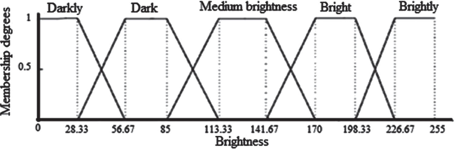

Rainfall attribute:

Considering the rainfall amounts given by the ONM in Algeria as listed in Table 1, four trapezoidal membership functions are considered to represent the fuzzy subsets of the CTD’s rainfall attribute, as given in Table 1 and Fig. 3. Hence, the number of FTD’s fuzzy items for the CTD’s rainfall attribute is four.

Table 1

Rainfall amount in Algeria

Fuzzy subset	Rainfall amounts in millimeter per hour (mm/h)
No rain	0
Low	]0,3]
Moderate	[4,7, 4,7]
High	≥ 8

Fig.3

Fuzzy subsets of the rainfall attribute with four Trapezoidal membership functions

Infrared channels attributes: For the rainfall attribute, the number of fuzzy subsets is defined by the experts (i.e., ONM), whereas its value for the visible channels attributes is determined according to the brightness knowledge of the MSG images (In our study, we propose five subsets). However, in the case of the infrared channel attributes, the number of fuzzy subsets is ambiguous because we do not have any expert information about its linguistic term sets. Hence, we need to use fuzzy algorithms to define the number of fuzzy subsets for each infrared channel attribute. In our study, the well-known FCM [30] algorithm and the validity index [32] are used to define the number of fuzzy subsets (clusters) for each CTD’s infrared attribute. The number of clusters is between a minimum number (C _min ≥ 2) and a maximum number (C _max), which are defined by the user. According to Bezdek [33], C _min = 2 and $C_{\max} = \sqrt{n}$ , where n is the number of elements, whereas in [34], C _min = 2 and C _max = 10. For each CDT’s infrared attribute IR _i, with the set of elements E _i = {x ₁, x ₂, … x _n}, i indicates the i-th infrared attribute, n is the number of E _i’s elements, and x _{t,(t=1,2…n)} is the pixel value of the t-th transaction for the IR _i attribute. We assign to IR _i, the number of clusters C _i, where C _i is an integer number in $[C_{\min}^{{IR}_{i}}, C_{\max}^{{IR}_{i}}]$ , and $C_{\min}^{{IR}_{i}}$ and $C_{\max}^{{IR}_{i}}$ represent the minimum number and the maximum number for IR _i, respectively. To define the optimal number of clusters C _i for each IR _i, the following steps are followed.

Step 1. For C _i= $C_{\min}^{{IR}_{i}}$ to $C_{\max}^{{IR}_{i}}$ do

Step 1.1 Apply the FCM algorithm using the inputs C _i and E _i.

Step 1.2 Calculate the validity index (V _{C
_i}) [32].

Step 2. The optimal number of clusters C _i is related to the V _{C
_i} with the maximum value.

3.2.2 Fuzzy item value definition

The following two notations are considered:

[VR, FS] is a fuzzy item for the visible/rainfall attribute VR with its associated fuzzy subset FS. For example, [VIS0.6, Brightly] is a fuzzy item for the visible attribute VIS0.6 with its associated fuzzy subset ‘Brightly’.

[IR, C (cr)] is a fuzzy item for the infrared attribute IR with its associated fuzzy subset C, where cr is a real value that represents the center value of the cluster C. For example, [IR12.0, C2 (47.28)] is the fuzzy item for the attribute IR12.0 related to the cluster C2, which has the center value of 47.28.

To calculate the membership degrees of each [VR, FS], we use 5 trapezoidal membership functions (see Fig. 2) for each VR ∈ VIS0.6, VIS0.8, NIR1.6 and 4 trapezoidal membership functions (see Fig. 3) for the rainfall attribute. While, for evaluating the membership degrees of each [IR, C (cr)], the FCM algorithm is used.

3.3 Fuzzy association rule extraction

Our aim is to extract fuzzy association rules in condition ⇒ conclusion form, where the right part (conclusion) of each generated rule has only one fuzzy item, which is described as [rainfall, FS], where FS ∈ {no-rain, low, moderate, high } are the fuzzy subsets associated with the rainfall item. To extract these fuzzy association rules, two steps should be followed. First, an extended version of the apriori algorithm [25] is used to find the list of the frequent fuzzy itemsets from the created fuzzy transactional database FTD. Second, the fuzzy association rules are generated using the found frequent fuzzy itemsets. The descriptions of these two steps are presented in the following subsections.

3.3.1 Identification of frequent fuzzy itemsets

To find the list of frequent fuzzy itemsets (LFFI), we adopt the apriori algorithm in our fuzzy rainfall estimation. Originally the canonical apriori algorithm is introduced to deal with crisp itemsets. However, in our method, the items are described as fuzzy items. Hence, the canonical apriori algorithm needs to be extended, where its crisp support formula is replaced by the defined fuzzy-based formula, which is given in Equation (3). The extended version of the original apriori algorithm, which is called fuzzy apriori algorithm, is given in pseudocode format in Algorithm 1.

Algorithm 1 fuzzy apriori algorithm

Input:

- FTD: The fuzzy transactional database.

- Mfs: The minimum fuzzy support.

- α-cut: The minimum threshold of membership in a fuzzy subset.

Output:

- LFFI: list of frequent fuzzy itemsets.

1: L ₁ ={Frequent fuzzy 1-itemsets}

2: for (k = 2; L _k-1≠ ∅; k++) do

3: C _k ← apriori - gen (L _k-1) ⊳Candidates of fuzzy K-itemsets.

4: for all transaction t ∈ FTD do

5: C _t = subset (C _k, t, α - cut)

6: for all candidates c ∈ C _t do

7: c . supp = + ⊤ (α _X (t [A])) ⊳ ⊤ (α _X (t _i [A])): is the minimum fuzzy value for the membership degrees of the fuzzy items (A,X) relating to the fuzzy itemset c in the transaction t.

8: end for

9: end for

10: $L_{k} = {c \in C_{k} | \frac{c . supp}{| T |} > = Mfs}$ ( |T|: is the total number of FTD’s transactions.

11: end for

12: LFFI = ⋃ _k L _k

As shown from this algorithm, the frequent fuzzy 1-itemset is generated in line 1 by calculating the fuzzy support for each fuzzy item of FTD, and only keep those fuzzy items that satisfy the minimum fuzzy support (Mfs). After that, steps 2 to 10 are repeated until the stopping criterion is stratified (i.e. L _k =∅). In each iteration cycle k of this algorithm, the function apriori - gen (L _k-1) generates a set of candidate fuzzy k-itemsets denoted as C _k through the joining of the previous frequent fuzzy (k-1)-itemsets L _k-1 with itself. In the C _k set, we delete each fuzzy itemset c, which has not a frequent fuzzy subset with k - 1 length in the L _k-1 set, and we prune also the not valid fuzzy itemsets. In order to find the L _k set from the C _k set, at first, for each transaction t from the FTD database, a set of fuzzy itemset C _t is created from C _k by considering only the C _k’s fuzzy itemsets, which satisfy the minimum threshold of membership in a fuzzy subset (α-cut) threshold. At second, for each c ∈ C _t we calculate its fuzzy support c . supp and finally the L _k is created by saving just the c fuzzy itemsets that have c . supps greater or equal than Mfs.

To clarify the aforesaid fuzzy apriori algorithm, the example of Figure 4 describes how to find the frequent fuzzy itemsets LFFI = ∪ _k L _k. Given the FTD as shown in Figure 4 where the first column indicates the number of the FTD’s transaction and the other columns of this table represent three items (Item 1, Item 2 and Item 3) which are associated with their fuzzy subsets (FS1.1 to FS3.2). The two parameters Mfs and α-cut are set with the values of 0.25 and 0.5 respectively. The first step is to find the 1-fuzzy itemset (L ₁), which contains all the fuzzy items of the candidate list C ₁ where their fuzzy support are greater than Mfs (i.e. The non frequent fuzzy itemsets of C ₁ with gray colors are not considered to generate L ₁). Next, each C _k, k = 2, 3, . . is generated using its list of frequent fuzzy itemsets l _k-1. For example the candidate list C ₂ is produced by performing the join operation between the fuzzy set L ₁ and itself (i.e. C ₂ = L ₁ ⋈ L ₁ = {(1) , (4) , (6) , (7)} ⋈ {(1) , (4) , (6) , (7))} = {(1 4) , (1 6) , (1 7) , (4 6) , (4 7) , (6 7)}), however the last fuzzy itemset (6 7) is not a valid fuzzy itemsets (i.e. See the cell drawn using a thin dashed border) because the two fuzzy itemsets 6 and 7 have the same attribute Item3. Therefore we prune it from C ₂. To find L ₂, we calculate the fuzzy supports of C ₂ (e.g), after that L ₂ is created by adding to it those fuzzy itemsets from C ₂, where their FSs ≥Mfs. The same aforesaid process (Join and Prun) is applied to generate C ₃ by using L ₂, where the fuzzy itemset (1 6 7) is omitted from C ₃ because it is not a valid fuzzy itemset. Furthermore, the fuzzy itemset (1 4 7) (See the cell drawn using a bold dashed border) is also removed because it contains a fuzzy itemset (4 7), which is not a member of L ₂. As result LFFI = L ₁ ∪ L ₂ ∪ L ₃ = {(1) , (4) , (6) , (7)} ∪ {(1 4) , (1 6) , (1 7) , (4 6)} ∪ {(1 4 6)}.

Fig.4

An example of generating the list of fuzzy frequent itemsets using the fuzzy apriori algorithm

3.3.2 Fuzzy association rule extraction

To extract the list of fuzzy association rules (LFAR), Algorithm 2 is used to generate this list from LFFI, which is created by fuzzy apriori algorithm 1.

Algorithm 2 fuzzy association rules extraction.

Input:

- LFFI: list of frequent fuzzy itemsets.

- Mfc: The minimum fuzzy confidence.

- α-cut: The minimum threshold of membership in a fuzzy subset.

Output:

- LFAR: list of fuzzy association rules.

1: for each frequent fuzzy k-itemsets L _k ∈ LFFI where k ≥ 2 do

2: for each fuzzy itemset (A, X) ∈ L _k do

3: if ∃ [rainfall, FS] ∈ (A, X) then ⊳ FS ∈ {low, moderate, high, no-rain}.

4: Generate the fuzzy association rule FAR from (A, X) as follows: (A, X) - [rainfall, FS] ⇒ [rainfall, FS]

5: Calculate the confidence Conf _FAR of FAR using equation (5)

6: if Conf _FAR ≥ Mfc then

7: LFAR = LFAR ⋃ FAR

8: end if

9: end if

10: end for

11: end for

As shown from the pseudo-code format of the fuzzy association rules extraction given in Algorithm 2, we take only the fuzzy itemsets (A, X) of the lists L _k with k ≥ 2 and contains the fuzzy item [rainfall, FS], where A represents the list of the used attributes, X indicates their associated fuzzy subsets and FS = {low, moderate, high, no-rain} are the fuzzy subsets associated with the rainfall item. For each taken itemset (A, X), generates its fuzzy association rule FAR as follows: (A, X) - [rainfall, FS] ⇒ [rainfall, FS] and calculates its fuzzy confidence Conf _FAR. If Conf _FAR ≥ Mfc, we add FAR to the final list LFAR, where Mfc is the minimum fuzzy confidence, which is defined by the user.

Given the list LFFI = L ₁ ∪ L ₂ ∪ L ₃ = {(1) , (4) , (6) , (7)}∪ {(1 4) , (1 6) , (1 7) , (4 6)} ∪ {(1 4 6)}, which is generated by the fuzzy apriori algorithm for the example shown in figure 4, and considering Item2 as the rainfall attribute, where their associated fuzzy subsets are FS2.1, FS2.2 and FS2.3; hence the fuzzy items including the attribute rainfall are [Item2, FS2.1], [Item2, FS2.2] and [Item2, FS2.3] which are represented by the numbers 3, 4 and 5 respectively. From LFFI, only the frequent fuzzy itemsets (A, X)s= {(1 4) , (4 6) , (1 4 6)} are considered to generate the fuzzy association rules, because L ₁ is a fuzzy 1-itemsets list and (1 6) , (1 7) are fuzzy 2-itemsets that do not contain at least one of the fuzzy items described by the numbers 3, 4 and 5. Herein, the generated fuzzy association rules are FARs={1 ⇒4, 6 ⇒ 4, (1 ∧6) ⇒4}, where ∧ indicates the fuzzy conjunction operator. As seen from this list, each FAR is generated from its related (A, X) by assigning to the right part (conclusion) of the FAR only one fuzzy item, which is [rainfall, FS] and the left part (condition) of FAR are all the fuzzy items of the associated (A, X) except for the fuzzy item, which is given to the conclusion part of this FAR. For instance, (1 ∧6) ⇒4 is a FAR generated from the fuzzy itemset (1 4 6), where its conclusion is the fuzzy item [Item2, FS2.2], which is represented by the number 4. By using equation (5), where Mfc = 0.65 and α-cut=0.5, the confidences of each generated FAR are calculated and only the FARs that have confidences greater or equal than the defined Mfc are considered to construct the final list LFAR. The confidence values of the generated FARs for the aforesaid example are: Conf _1⇒4 = 0.68, Conf _6⇒4 = 0.59 and Conf _(1∧6)⇒4 = 0.84; therefore LFAR = {1 ⇒ 4, (1 ∧6) ⇒4}.

4 Experimental results

In this section, to verify and validate the effectiveness of our proposal, two real databases are used. the first one is adopted to train (learn) the proposed model (fuzzy association rules), and the second one is used to validate the trained model. The description of the used databases is given in the Data sets subsection. Then, the trained model is presented in the subsection model construction. In the final subsection (Model validation), we validate the generated model by performing an effective comparison against MPE, which is a very useful product for estimating rainfall.

4.1 Data sets

In our study, we select the northeastern region of Algeria for rainfall estimation because it is the most precipitous region according to the ONM. It is located between 34.5° Northern and 37° Northern, and between 3.5° Western and 9° Eastern. Two databases are considered to create and validate the proposed model for estimating the rainfall of the selected region. For this reason, the databases are created by collecting the SEVIRI’s images from 11 of the multispectral channels of the MSG satellite (except for the HRV channel) and the images of the MPE product. In our study, we choose the rainy period to collect the aforesaid images, which are collected from October 1,2016 to March 31, 2017, where the images are acquired every 15 min from 8:00 to 16:00. For each hour, the first database (denoted as TrainDB), which is used to train the developed model, is created by assigning to TrainDB the images acquired in the minutes (00, 15, 30). Meanwhile, the second database (denoted as ValidDB), which is used for validating our proposal, is constructed by recording to ValidDB the images acquired at 45 min.

4.2 Model construction

To extract the list of fuzzy association rules (model), the database TrainDB is used to learn the constructed model. The FCM [30] algorithm and the validity index [32] are used together to define the number of the fuzzy subsets for the infrared attributes, and their fuzzy values. The FCM’s parameters are set as follows. The used distance is the Euclidean distance, the fuzziness exponent m = 2, and the stopping criterion epsilon ξ = 0.001. The C _min and the C _max parameters are initialized with values of 4 and 10, respectively. The generated model is constructed using the fuzzy apriori algoithm given in Algorithm 1 and the fuzzy association rule extraction given in Algorithm 2; their parameter settings are as follows: the minimum fuzzy support Mfs = 0.1, the minimum fuzzy confidence Mfc = 0.7, and the minimum threshold of membership in a fuzzy subset α-cut = 0.67.

Table 2
Fuzzy supports for each fuzzy item of the rainfall attribute

Fuzzy item Fuzzy support

[rainfall, high] 0.02

[rainfall, moderate] 0.04

[rainfall, low] 0.36

[rainfall, no-rain] 0.56

Fuzzy item	Fuzzy support
[rainfall, high]	0.02
[rainfall, moderate]	0.04
[rainfall, low]	0.36
[rainfall, no-rain]	0.56

In the fuzzy apriori algorithm, we start by generating the 1-itemsets list (L ₁), which contains the first list of the fuzzy frequent items. This list is determined by taking only the fuzzy items with fuzzy supports higher than the defined Mfs. In our study, to have fuzzy association rules in the form of condition⇒ [rainfall,FS], where FS ∈ {no-rain, low, moderate, high}, the list L ₁ should have all the fuzzy items of the rainfall attribute. However, and especially for our region study, the frequency value of the rain precipitation with a high or moderate levels is very small compared with the frequency value of the low or no-rain precipitation levels. Therefore, the fuzzy supports of the two fuzzy items [rainfall, moderate] and [rainfall, high] have very low values compared with the fuzzy supports of the [rainfall, low] and [rainfall, no-rain] fuzzy items. For instance, as shown in Table 2, which represents the fuzzy supports for the fuzzy items of the rainfall attribute given by performing our proposed method on TrainDB, the fuzzy support values of the two fuzzy items [rainfall, moderate] = 0.04 and [rainfall, high] = 0.02, which are less than the Mfs = 0.1 (not frequent fuzzy items); thus, fuzzy association rules in the form of condition ⇒ [rainfall,moderate] or condition ⇒ [rainfall,high] cannot be obtained.

To solve this problem and to construct a model with a list of fuzzy association rules that can decide from each pixel (database’s transaction) its related rainfall fuzzy subset (i.e., no-rain, low, moderate and high), we need to generate four sublists of fuzzy association rules for each rainfall fuzzy item. The final list of the fuzzy association rules (LFAR) for the constructed model is the regrouping of these generated fuzzy sublists. The initial fuzzy database is denoted as FtrainDB, which is provided from the TrainDB by running our proposed method. The following steps are performed to generate (LFAR).

Step 1. For i =1 to 4 do //where i represents the index value of each generated fuzzy sublist.

Step 2. Calculate the fuzzy supports for the fuzzy items of the rainfall attribute.

Step 3. Sort in ascending order the fuzzy items of the rainfall attribute according to their fuzzy support values.

Step 4. Generate the fuzzy sublist of the fuzzy association rules SL _i of the fuzzy item rainfall, which has the greatest fuzzy support by performing Algorithms 1 and 2 on the FtrainDB, where the Mfs and Mfc parameters are set with new values.

Step 5. Update the FtrainDB by eliminating the transactions of this fuzzy item that have degrees of membership greater than α-cut.

Step 6. LFAR = LFAR ⋃ SL _i

Tables 3–6 represent the four fuzzy sublists of the constructed model (i.e., LFAR). In our study, to select the rainfall fuzzy subset for any transaction of the validated database, the rules are checked from the first fuzzy sublist (SL ₁) to the last one (SL ₄), and the first verified fuzzy association rule is applied to define the fuzzy subset of this transaction.

Table 3

List of the fuzzy association rules for the fuzzy item [rainfall, no-rain] with Mfs = 0.14 and Mfc = 0.74.

Fuzzy association rule	Fuzzy support	Fuzzy confidence
21∧36 ⇒ 60	0.156	0.747
21∧40 ⇒ 60	0.155	0.769
21∧48 ⇒ 60	0.168	0.766
21∧52 ⇒ 60	0.173	0.759
21∧56 ⇒ 60	0.153	0.745
36∧40 ⇒ 60	0.143	0.757
36∧48 ⇒ 60	0.164	0.756
36∧52 ⇒ 60	0.175	0.754
36∧56 ⇒ 60	0.167	0.748
40∧48 ⇒ 60	0.198	0.775
40∧52 ⇒ 60	0.176	0.769
48∧52 ⇒ 60	0.203	0.766
48∧56 ⇒ 60	0.161	0.752
52∧56 ⇒ 60	0.174	0.751
21∧40∧48 ⇒ 60	0.145	0.768
21∧48∧52 ⇒ 60	0.155	0.760
36∧40∧48 ⇒ 60	0.141	0.757
36∧48∧52 ⇒ 60	0.160	0.755
36∧48∧56 ⇒ 60	0.147	0.751
36∧52∧56 ⇒ 60	0.158	0.750
40∧48∧52 ⇒ 60	0.175	0.769
48∧52∧56 ⇒ 60	0.159	0.752
36∧48∧52∧56 ⇒ 60	0.146	0.750

Fuzzy items labeling: 21:[NIR1.6,dark], 36:[WV7.3,C4(63.830)], 40:[IR8.7,C4(73.203)] 48:[IR10.8,C4(71.075)],52:[IR12.0,C4(68.569)], 56:[IR13.4,C4(60.506)] 60:[Rainfall, no-rain]

Table 4

List of the fuzzy association rules for the fuzzy item [rainfall, low] with Mfs = 0.12 and Mfc = 0.95.

Fuzzy association rule	Fuzzy support	Fuzzy confidence
12∧21 ⇒ 57	0.195	0.958
18∧31 ⇒ 57	0.135	0.984
21∧31 ⇒ 57	0.198	0.971
21∧35 ⇒ 57	0.150	0.957
21∧47 ⇒ 57	0.137	0.968
21∧51 ⇒ 57	0.131	0.964
21∧55 ⇒ 57	0.141	0.958
31∧35 ⇒ 57	0.148	0.970
31∧55 ⇒ 57	0.141	0.968
35∧47 ⇒ 57	0.131	0.967
35∧51 ⇒ 57	0.138	0.965
35∧55 ⇒ 57	0.150	0.962
39∧47 ⇒ 57	0.125	0.987
47∧51 ⇒ 57	0.155	0.971
47∧55 ⇒ 57	0.128	0.965
51∧55 ⇒ 57	0.140	0.964
35∧47∧51 ⇒ 57	0.120	0.966
47∧51∧55 ⇒ 57	0.122	0.965

Fuzzy items labeling: 12:[VIS0.6, medium bright],18:[VIS0.8, bright], 21:[IR1.6, dark] 31:[WV6.2, C3(48.667)],35:[WV7.3, C3(55.399)],39:[IR8.7, C3(63.396)] 47:[IR10.8, C3(61.174)],51:[IR12.0, C3(58.792)], 55:[IR13.4, C3(52.706)] 57:[Rainfall, low]

Table 5

List of the fuzzy association rules for the fuzzy item [rainfall, moderate] with Mfs = 0.12 and Mfc = 0.8.

Fuzzy association rule	Fuzzy support	Fuzzy confidence
30∧50 ⇒ 58	0.152	0.811
30∧54 ⇒ 58	0.168	0.819
30∧34∧46 ⇒ 58	0.124	0.805
30∧34∧50 ⇒ 58	0.137	0.815
30∧34∧54 ⇒ 58	0.142	0.820
30∧46∧54 ⇒ 58	0.125	0.803
30∧50∧54 ⇒ 58	0.144	0.814
30∧34∧46∧50 ⇒ 58	0.120	0.806
30∧34∧50∧54 ⇒ 58	0.132	0.817
30∧46∧50∧54 ⇒ 58	0.123	0.804

Fuzzy items labeling: 30:[WV6.2, C2(41.189)], 34:[WV7.3,C2(45.983)], 46:[IR10.8, C2(49.931)] 50:[IR12.0, C2(47.281)],54:[IR13.4, C2(43.738)], 58: [Rainfall, moderate]

Table 6

List of the fuzzy association rules for the fuzzy item [rainfall, high] with Mfs = 0.19 and Mfc = 0.65.

Fuzzy association rule	Fuzzy support	Fuzzy confidence
22∧33∧41 ⇒ 59	0.193	0.654
22∧37∧41 ⇒ 59	0.203	0.653
22∧41∧45 ⇒ 59	0.196	0.655
22∧41∧49 ⇒ 59	0.194	0.656
22∧33∧37∧41 ⇒ 59	0.192	0.653
22∧33∧41∧45 ⇒ 59	0.191	0.654
22∧33∧41∧49 ⇒ 59	0.190	0.654
22∧37∧41∧45 ⇒ 59	0.195	0.654
22∧37∧41∧49 ⇒ 59	0.193	0.655
22∧41∧45∧49 ⇒ 59	0.193	0.654
22∧33∧37∧41∧45 ⇒ 59	0.190	0.653
22∧37∧41∧45∧49 ⇒ 59	0.192	0.654

Fuzzy items labeling: 22:[NIR1.6, medium bright], 33:[WV7.3, C1(31.673)] 37:[IR8.7,C1(36.413)], 41:[IR9.7,C1(44.919)],45:[IR10.8,C1(33.617)] 49:[IR12.0,C1(30.129)], 59:[Rainfall,high]

Table 7

Number of pixels of each fuzzy item of the rainfall attribute for each α-cut

α-cut	Number of pixels	[rainfall, no-rain]	[rainfall, low]	[rainfall, moderate]	[rainfall, high]
	NP_MPE	233705	145017	12455	8231
0.80	NP_M	172635	144189	22187	4785
	NP_V	130125	101096	3006	3019
	NP_MPE	233705	145017	12713	8429
0.75	NP_M	189056	143734	23154	7006
	NP_V	141997	107691	4040	4448
	NP_MPE	233705	145017	15145	8429
0.70	NP_M	196901	142596	21265	7973
	NP_V	147502	111044	4783	5136
	NP_MPE	233705	145645	15355	8429
0.65	NP_M	201175	144545	25086	8932
	NP_V	150413	114186	6498	5517
	NP_MPE	233705	145645	17399	8577
0.60	NP_M	211581	145344	17998	9714
	NP_V	157322	120121	7405	5915
	NP_MPE	233705	145645	17399	8577
0.55	NP_M	223410	135800	17396	11145
	NP_V	165494	121336	7634	6215
	NP_MPE	233705	146134	17648	8577
0.50	NP_M	228945	134655	17426	11850
	NP_V	168754	124013	8531	6490

4.3 Model validation

To evaluate the performance of the proposed fuzzy rainfall estimation method, we compare the rainfall estimation results obtained applying the constructed model on ValidDB against the rainfall estimation results obtained by the MPE product on the same ValidDB database. Herein, the MPE product is chosen for validating our proposal, because it is ranked as the best rainfall estimator.

For each fuzzy subset of the rainfall attribute and by varying the α-cut value from 0.80 to 0.50 by a decreasing value of 0.05, we calculate the estimated number of pixels found by our method (NP_M), the estimated number of pixels found by the MPE product (NP_MPE), and the number of valid pixels obtained by our method (NP_V), where only the pixels that have degrees of membership greater than α-cut are considered. For each ValidDB’s transaction, a valid pixel is a pixel that has the same fuzzy subset as the pixel of the MPE image (i.e., good classification). The values of the calculated NP_M, NP_MPE, and NP_V for each α-cut are presented in Table 7.

The following accuracy metrics are used to validate our proposed method.

Average validation rate (AVR), which is calculated as follows. $AVR = \frac{\sum_{i = 1}^{n} NP_V_{i}}{\sum_{i = 1}^{n} NP_M_{i}}$ (8)

Root mean square error (RMSE), which is given in the following equation: $RMSE = \sqrt{\frac{\sum_{i = 1}^{n} (NP_M_{i} - NP_M {PE}_{i})^{2}}{n}}$ (9)

For each α-cut, we search for the one that maximizes the validation rate and, at the same time, the one that minimizes the estimation error. We calculate for each α-cut the average validation rate and the root mean square error. The obtained results are shown in Table 8, and the two histograms, as shown in Fig. 5 and Fig. 6, present the root mean square error and the average validation rate for each α-cut, respectively.

Table 8

The average validation rate and the root mean square error for each α-cut

α-cut	RMSE	AVR
0.80	30971.02	0.69
0.75	22946.77	0.71
0.70	18695.30	0.72
0.65	16265.00	0.73
0.60	11062.00	0.75
0.55	5147.50	0.77
0.50	6426.25	0.78

Fig.5

Root mean square error for each α-cut

Fig.6

The average validation rate for each α-cut

Fig. 6 shows that by varying the value of α-cut from 0.80 to 0.50 at 0.05 decrements, the value of the average validation is found to be higher than 0.69, which is an interesting value. Furthermore, as shown in Fig. 5, for the α-cut values lying in the range [0.50, 0.55], the mean squared error is with a low value compared with other values of α-cuts. Moreover, the best α-cut value that allows our method to obtain the best model is α-cut=0.55.

5 Conclusion and prospects

In this study, we present a new method for estimating rainfall using images from 11 MSG satellite spectral channels. The proposed method is based on the use of fuzzy association rules. Our method offers a reliable estimate of precipitation over Northeastern Algeria through the use of a large amount of diverse data from 11 channels and the introduction of fuzziness, which enables us to process these uncertain data in a flexible manner and estimate the intensity of rain in four fuzzy classes (no-rain, low, moderate, and high). Furthermore, our method can be applied to estimate rainfall during day and night. For night precipitation estimation, we use only the infrared channels’ data. The comparison of our proposed method’s and the MPE product’s results demonstrate and verify the validity of the generated model (fuzzy association rules) by our proposed method.

In the current study, the HRV channel data are not considered for estimating rainfall. Hence, in the future, we will consider relevant meteorological data other than those used in the current work, such as pressure, and wind speed, in the rainfall estimation process for improved precipitation estimation.

Footnotes

Acknowledgements

We express our deepest appreciation to all those who provided us the possibility to complete this report. We are sincerely grateful to the Editor-in-Chief for their valuable suggestions and encouragement, and to the reviewers for their comments, which further enhanced our manuscript. Furthermore we would like to thank the staff of the Remote Sensing Section from Space of Royal Meteorological Institute of Belgium for their crucial role in this work. Finally, we want to offer a very special thanks to Dr. Nicolas CLERBAUX.

References

Carn

and Lahuec

J.P.

Estimation des précipitations au Niger au cours de la saison des pluies à partir de l’imagerie infrarouge Météosat: Bilan et critique des méthodes utilisées, Veille Climatique Satellitaire 17 (1987), 40–48.

Arkin

P.A.

and Meisner

B.N.

The relationship between largescale convective rainfall and cold cloud over the western hemisphere during 1982-84, Monthly Weather Review 115(1) (1987), 51–74.

Adler

R.F.

, Negri

A.J.

A satellite infrared technique to estimate tropical convective and stratiform rainfall, Journal of Applied Meteorology 27(1) (1988), 30–51.

Guillot

L’utilisation des satellites météorologiques pour l’estimation de la pluie en zone sahélo-soudanienne au Centre de Météorologie Spatiale de Lannion, 1990.

Levizzani

, Schmetz

, Lutz

H.J.

, Kerkmann

, Alberoni

P.P.

and Cervino

Precipitation estimations from geostationary orbit and prospects for METEOSAT Second Generation, Meteorological Applications.(Cambridge University Press) 8(1) (2001), 23–41.

Bergès

J.C.

, Jobart

, Chopin

and Roca

EPSATSG, a satellite method for precipitation estimation, 2009.

Yin

Z.Y.

, Liu

, Zhang

and Chung

C.F.

Using a geographic information system to improve Special Sensor Microwave Imager precipitation estimates over the Tibetan Plateau, Journal of Geophysical Research: Atmospheres(Wiley Online Library) 109(D3) (2004).

Marzano

F.S.

, Palmacci

, Cimini

, Giuliani

and Turk

F.J.

Multivariate statistical integration of satellite infrared and microwave radiometric measurements for rainfall retrieval at the geostationary scale, IEEE Transactions on Geoscience and Remote Sensing(IEEE) 42(5) (2004), 1018–1032.

Jobard

and Desbois

Satellite estimation of the tropical precipitation using the METEOSTAT and SSM/I data, Atmospheric Research(Elsevier) 34(1-4) (1994), 285–298.

10.

Jobard

Status of satellite retrieval of rainfall at different scales using multi-source data, Proc MEGHA-TROPIQUES 2nd Scientific Workshop 2001.

11.

Torricella

, Levizzani

and Celano

Applications of a rainfall estimation technique based onMWand IR satellite data: Assessment of reliability of instantaneous rain rate maps in the mediterranean, Institute of Atmospheric Sciences and Climate, National Research Council (2003), 1–6.

12.

Schmetz

, Pili

, Tjemkes

, Just

, Kerkmann

, Rota

and Ratier

An introduction to Meteosat second generation (MSG), Bulletin of the American Meteorological Society (American Meteorological Society) 83(7) (2002), 977–992.

13.

Lazri

, Ameur

, Brucker

J.M.

, Testud

, Hamadache

, Hameg

, Ouallouche

and Mohia

Identification of raining clouds using a method based on optical and microphysical cloud properties from Meteosat second generation daytime and nighttime data, Applied Water Science (Springer) 3(1) (2013), 1–11.

14.

Ouallouche

and Ameur

Rainfall detection over northern Algeria by combining MSG and TRMM data, Applied Water Science (Springer) 6(1) (2016), 1–10.

15.

Bensafi

, Lazri

and Ameur

Novel WkNN-based technique to improve instantaneous rainfall estimation over the north of Algeria using the multispectral MSG SEVIRI imagery, Journal of Atmospheric and Solar-Terrestrial Physics (Elsevier) 183 (2019), 110–119.

16.

Ouallouche

, Lazri

and Ameur

Improvement of rainfall estimation from MSG data using Random Forests classification and regression, Atmospheric Research. (Elsevier) 211 (2018), 62–72.

17.

Thies

and Nauß

ß and J. Bendix, Discriminating raining from non-raining clouds at mid-latitudes using meteosat second generation daytime data, Atmospheric Chemistry and Physics (Copernicus GmbH) 8(9) (2008), 2341–2349.

18.

Thies

, Nauss

and Bendix

Delineation of raining from non-raining clouds during nighttime using Meteosat-8 data, Meteorol Appl 15 (2008), 219–230.

19.

Roebeling

R.A.

and Holleman

Validation of rain rate retrievals from SEVIRI using weather radar observations, Proc EUMETSAT Meteorological Satellite Conference, Citeseer (2008), pp. 8–11.

20.

Feidas

and Giannakos

Identifying precipitating clouds in Greece using multispectral infrared Meteosat Second Generation satellite data, Theoretical and Applied Climatology (Springer) 104(1-2) (2011), 25–42.

21.

Feidas

and Giannakos

Classifying convective and stratiform rain using multispectral infrared Meteosat Second Generation satellite data, Theoretical and Applied Climatology (Springer) 108(3-4) (2012), 613–630.

22.

Zadeh

L.A.

Fuzzy sets, Information and Control 8(3) (1965), 338–353 New York.

23.

Cock

M.D.

, Cornelis

and Kerre

E.E.

Elicitation of fuzzy association rules from positive and negative examples, Fuzzy Sets and Systems 149(1) (2005), 73–85 (Elsevier).

24.

Agrawal

, Imieliński

and Swami

Mining association rules between sets of items in large databases, Acm Sigmod Record (ACM) 22(2) (1993), 207–216.

25.

Agrawal

and Srikant

and others, Fast algorithms for mining association rules, Proc 20th Int Conf Very Large Data Bases, VLDB 1215 (1994), pp. 487–499.

26.

Delgado

, Marín

, Sánchez

and Vila

M.A.

Fuzzy association rules: General model and applications, IEEE Transactions on Fuzzy Systems (IEEE) 11(2) (2003), 214–225.

27.

Dubois

, Hüllermeier

and Prade

A systematic approach to the assessment of fuzzy association rules, Data Mining and Knowledge Discovery (Springer) 13(2) (2006), 167–192.

28.

Hong

T.P.

, Lin

K.Y.

and Wang

S.L.

Fuzzy data mining for interesting generalized association rules, Fuzzy Sets and Systems (North-Holland) 138(2) (2003), 255–269.

29.

Djouadi

and Radaoui

Découverte de règles d’association: Application aux Données imprécises, Logique floue et ses applications. Toulouse, France, 2006, pp. 195–202.

30.

Bezdek

J.C.

Objective function clustering, Pattern recognition with fuzzy objective function algorithms. (Springer), 1981, pp. 43–93.

31.

Seddi

and Ameur

Estimation des precipitations en utilisant L’information multispectrale du satellite meteosat, Larhyss Journal (ASJP) 8(2) (2010), 179–193.

32.

Bezdek

J.C.

Cluster validity with fuzzy sets, Journal of Cybernetics (Taylor & Francis) 3(3) (1974), 58–73.

33.

Pal

N.R.

and Bezdek

J.C.

On cluster validity for the fuzzy c-means model, IEEE Transactions on Fuzzy Systems (IEEE) 3(3) (1995), 370–379.

34.

Bouguessa

, Wang

and Sun

An objective approach to cluster validation, Pattern Recognition Letters (Elsevier) 27(13) (2006), 1419–1430.

Rainfall estimation from MSG images using fuzzy association rules

Abstract

Keywords

1 Introduction

2 Basic notions

2.1 Association rules

3.2.1 Fuzzy item number definition

3.3 Fuzzy association rule extraction

3.3.1 Identification of frequent fuzzy itemsets

4 Experimental results

4.1 Data sets

4.2 Model construction

Table 2 Fuzzy supports for each fuzzy item of the rainfall attribute Fuzzy item Fuzzy support [rainfall, high] 0.02 [rainfall, moderate] 0.04 [rainfall, low] 0.36 [rainfall, no-rain] 0.56

Footnotes

Acknowledgements

References

Table 2
Fuzzy supports for each fuzzy item of the rainfall attribute

Fuzzy item Fuzzy support

[rainfall, high] 0.02

[rainfall, moderate] 0.04

[rainfall, low] 0.36

[rainfall, no-rain] 0.56