A Bayesian approach to incomplete fuzzy reciprocal preference relations in consensus reaching process and its application in project performance evaluations

Abstract

Due to the fact that individual knowledge is often inadequate and deficient in group decision-making problems, it is commonly seen that the preference information provided by the decision makers are incomplete. To encounter this problem lots of relevant researches have already been carried out. However, previous methods often only take into account either the information of the expert who provided incomplete preference, or information provided by the rest of the group. To be more thorough and comprehensive, this paper combined both parts of the information, by first setting the unknown preference values as output and known ones as inputs, training the Bayesian regression model with the complete observations of other experts to detect the associations between them, and then putting in the incomplete preference information to predict the unknown ones. Moreover, inspired by the empirical rule of the Gaussian distribution, this paper also propose to combine the concept of confidence interval with that of interval-valued preference relations, by expressing the prediction results with interval-valued fuzzy reciprocal relations to allow some degree of uncertainty. On the basis of that an iterative consensus reaching process incorporated with feedback mechanism is also proposed. Finally a case study of possible application of our proposed model in project performance evaluations is carried out, the results of which then further verify the practicality and validity of our model.

Keywords

Group decision making incomplete fuzzy reciprocal preference relation Bayesian linear regression consensus reaching process

1 Introduction

Group Decision Making (GDM) [11 , 40] is typically described as the cognitive process where a group of Decision Makers (DM), sometimes also referred to as experts, are gathered to collectively select the best alternative or alternatives from a set of feasible ones, considering all the opinions and preferences expressed by the DMs.

One of the most prominent advantages of GDM is that the collective intellectual or wisdom of the group is always greater than that of any individual, thus it is safe to say that the solution obtained through GDM is usually more thoroughly considered and well justified. And since the GDM relies on the collective intellectual of the entire group, it does not and cannot require all individual to have a complete and unimpaired knowledge about all the alternatives under evaluation. As a consequence, sometimes it is inevitable that the opinions and preferences provided by certain DMs are incomplete [3 , 42], due to different types of reasons such as “limited expertise, domain complexity or even pressure in making a decision [15]”.

Various researches have been done regarding this issue. In [18] E. Herrera-Viedma et al. proposed an iterative procedure of estimating the unknown preference value based on the additive consistency property of the DM’s incomplete fuzzy preference relations. Alonso Sergio et al. in [2] put forward both the individual and social strategies of dealing with the situation of total ignorance where a DM does not provide any information about a particular alternative. Jian Wu et al. [37] proposed to estimate the unknown preference values based on the trust relationship of the experts obtained through a trust propagation algorithm. Qian Liang et al. [24] constructed a linear programming model to employ social ties as the bases of completing the missing preference value. Roughly speaking, these methods can be classified into two general categories: estimation methods based on consistency using only the preference information provided by the DM oneself [1 , 36], and ones based on Social Network Analysis (SNA) using the preference information of the other experts within the group [24, 37].

It is worth noting that the majority of the estimation methods that fall into the first category are mostly based on various type of consistency, including additive consistency [12 , 18], order consistency [9], multiplicative consistency [25] etc. This approach has several obvious advantages, one being that the estimation results would be compatible with the preference information the DM did provide, and another being that it does not require additional information about the nature of the relationship between the DMs. But this approach essentially assumes that the unknown preference value would be consistent, or at least as consistent as possible, with the other preference information, which may not be the case in practical applications where the preference relations provided by DMs are often inconsistent and contradictory.

As for the estimation methods of the second category, the question then arises on how the preference information provided by other DMs is utilized. In [37] Jian Wu et al. proposed to first compute the relative trust scores according to the trust relationship provided by the DMs, and then estimate the unknown 2-tuple linguistic preference values by aggregating the rest of the DMs’ decision matrices with the weighted arithmetic average operator where the RTSs constitute as the normalized weight vector. Whereas in [24] Qian Liang et al. proposed to use social network analysis methodologies to calculate the social ties’ strength of the DMs, then a linear programming is put forward with two objectives: one is to minimize the deviation between the estimated preference values and the weighted preferences of those DMs who have the strongest social ties to the DM under discussion, and the other is to minimize the inconsistency degree of the preference relation. It should be pointed out that these two methods share some clear similarities: for one thing, they both adopts the assumption that a person is more easily persuaded by the people who is socially closest to oneself; for another, both methods in essence estimate the unknown preference value by aggregating other DMs’ preference information with the weighted average operator. But there is one obvious disadvantage to these two methods, and that is they both require additional information regarding the social relationships of the DMs.

Another drawback of both of the categories is that they only take into account part of the preference reference information at hand: the consistency-based methods only make use of the information provided by one DM, while the SNA-based methods only make use of the information provided by the rest of the group. Therefore to be more thorough and comprehensive, this paper propose a new approach to estimate the unknown preference value based on Bayesian linear regression [10], which can utilize both parts of the preference information. If we take the preference values the DM did provide as inputs, and the unknown preference values as outputs, then a regression model can be constructed to predict the DM’s preferences when he or she is not able to provide one. The fundamental idea of this approach is as follows: we suppose that the preferences of one alternative over another is essentially a reflection of the DM’s evaluations of the alternatives over certain criterions, therefore there exists some kind of correlation or association between the preference values of one DM, which we proposed to detect through Bayesian linear regression.

It is worth mentioning that previous research [6] has in fact also adopted a Bayesian perspective in consensus building in the Analytic Hierarchical Process Group Decision Making (AHP-GDM) problems [32]. Although our method differs from it in various aspects, some reasons that made Bayesian linear regression model suitable for AHP-GDM problems also apply here. First, since in the classical fuzzy GDM scenarios the number of DMs is fairly small and the under-sample problem may occur, one advantage of Bayesian linear regression then emerges that it does not require a large amount of data samples, making it easier to utilize in practical applications. Second, the estimation results obtained through Bayesian linear regression model takes the form of probability distribution, which allows the DM to maintain some degree of doubt and uncertainty, making it easier for the DM to accept the completed preference relation as a fair representation of his or her original opinions.

Moreover, after the estimation of the unknown preference values is completed, in GDM there usually is a Consensus Reaching Process (CRP), in which the DMs can negotiate and gradually bring their positions closer to each other to finally reach a consensus solution. The CRP is of such great importance that it has been well studied in various GDM researches [5 , 41]. In this paper, we also propose a CRP model based on Bayesian linear regression. First the unknown preference values in the Incomplete Fuzzy Reciprocal Preference Relations (IFRPRs) provided by DMs are estimated with Bayesian linear regression; then we propose to represent the prediction results in the form of Interval-Valued Fuzzy Reciprocal Preference Relations (IVFRPRs); next the consensus level of each DM is calculated and the DMs with insufficient consensus levels are identified and revision advice is generated to help these DMs to reconsider their preferences; finally an exploitation phase is carried out to select the best alternative or alternatives from the feasible sets.

The rest of this paper is organized as follows: Section 2 briefly introduces some preliminary concepts of IFRPRs and Bayesian linear regression; in Section 3 the general Bayesian model for estimating the unknown preference values is constructed, the result of which is then proposed to be represented with IVFRPRs, and an illustrative example is carried out; in Section 4 said Bayesian model is utilized, and the complete process of consensus reaching with IVFRPRs is described; in Section 5 a numerical case study of our model’s application in project performance evaluations is carried out; finally Section 6 marks the end of this paper with some concluding remarks.

2 Preliminaries

2.1 Incomplete fuzzy reciprocal preference relations

Suppose there is a finite set of alternatives A = {a₁, a₂, . . . , a_M} (M ≥ 2), and a group of experts denoted as E = {e₁, e₂, . . . , e_N} (N ≥ 2) who are gathered to rank said alternatives from the best to the worst, according to their own individual knowledge of the task at hand. Each expert gives his or her preference information in the form of Fuzzy Reciprocal Preference Relation (FRPR), the formal definition of which is given below.

Definition 1. [28]A Fuzzy Reciprocal Preference Relation (FRPR) R on a finite set of alternatives A = {a₁, a₂, . . . , a_M} (M ≥ 2) is a fuzzy set on the product set A × A, which is characterized by a membership function π_R : A × A → [0, 1], with π_R (a_i, a_j), = r_ij, verifying r_ij + r_ji = 1, ∀ i, j = 1 : M.

When the number of alternatives M is small enough, the FRPR is often expressed in the form of a M × M matrix: $R = {[\begin{matrix} 0.5 & r_{12} & \dots & r_{1 M} \\ r_{21} & 0.5 & \dots & r_{2 M} \\ ⋮ & ⋮ & ⋱ & ⋮ \\ r_{M 1} & r_{M 2} & \dots & 0.5 \end{matrix}]}_{M \times M}$ (1) where r_ij can be interpreted as the degree to which alternative a_i is preferred over a_j. r_ij = 1 indicates that alternative a_i is strictly preferred over a_j; r_ij ∈ (0.5, 1) indicates that alternative a_i is at least as good as a_j; and r_ij = 0.5 indicates that a_i and a_j are indifferent to the DM. Naturally we would have that r_ii = 0.5, ∀i = 1 : M.

The usual GDM problem often assumes that the preference relations provided by the experts are complete and satisfactory, which may not be true in certain circumstances. Individual knowledge of the question under evaluation is, more often than not, inadequate and deficient. And as a result, in practical applications, some expert may not be able to provide his or her preference information on certain pair of alternatives. It is worth noting that the lack of a preference value is not equivalent to complete indifference between the alternatives, therefore it is of great importance to employ an appropriate method to estimate the missing preference value. And in order to do that, here we first give the formal definition of Incomplete Fuzzy Reciprocal Preference Relation (IFRPR).

Definition 2. [18]A function f : X → Y is called partial when not every element in the set X necessarily maps onto an element in the set Y. When every element from the set X maps onto one element of the set Y then we have a total function.

Definition 3. [18] An Incomplete Fuzzy Reciprocal Preference Relation (IFRPR)R on a set of alternatives A is a fuzzy set on the product set A × A that is characterized by a partial membership function.

Example 1. Here we give a simple illustrative case of IFRPR, as shown below: $R = [\begin{matrix} 0.5 & 0.25 & 0.85 & 0.3 \\ 0.75 & 0.5 & ? & 0.15 \\ 0.15 & ? & 0.5 & 0.35 \\ 0.7 & 0.85 & 0.65 & 0.5 \end{matrix}]$ where r₂₃ and r₃₂ are unknown because the expert is unable to provide his or her opinions regarding the preference of alternative a₂ over a₃. Here we denote the unknown preference values with the question mark “?” [24], in other research papers it has also been denoted as “×” [3].

2.2 Bayesian linear regression

The main purpose of this subsection is to introduce the basic concepts of Bayesian linear regression [8, 10] for its later utilization in estimating the missing value in IFRPRs.

The general goal of regression can be briefly described as: given a data set compromising N′ observations { x _i|i = 1 : N′} together with their corresponding target values {t_i|i = 1 : N′}, the task is to train a model that can predict the value of t given a new predictor x . And rather than constructing a proper function t = f ( x ) that gives precise target value for new predictors, Bayesian linear regression method takes the probabilistic perspective and gives the prediction results in the form of probability distribution.The general approach of Bayesian linear regression can be simplified as: first we formulate our knowledge about the world with a probabilistic model, where the parameters are unknown; then we express our assumptions, or prior beliefs about the unknown parameters by specifying the prior distribution over these parameters; next we observe the given data, and compute the posterior distribution of the parameters given the observed data; at last we can make predictions by integrating over the posterior distribution.

Following these steps, first we formulate our knowledge about the regression problem at hand. Here we assume that the target value t is generated by a deterministic linear function with additive Gaussian noise, namely $t = \sum_{k = 1}^{K} w_{k} φ_{k} (x) + ɛ = w^{T} φ (x) ≜ y (x, w) + ɛ$ (2) where w = (w₁, . . . , w_K) ^T is the unknown weight vector of regression;ɛis a zero mean Gaussian noise with precision β, which is to say, $ɛ \sim N (0, β^{- 1})$ ; and φ ( x ) = (φ₁ ( x ) , . . . , φ_K ( x )) is known as basic function. Usually the simplest form of basic function is φ ( x ) = x , but other forms of basic functions can also be utilized to model more complex functions. Then from Equation (2) we could write $P (t | x, w, β) = N (t | y (x, w), β^{- 1})$ (3)

Now for a data set compromising of input predictors $X = {x_{1}, . . ., x_{N^{'}}}$ with their corresponding target values t = (t₁, . . . , t_N′) ^T, we assume that these samples are drawn independently from the distribution in Equation (3), then the likelihood can be written as $P (t | X, w, β) = \prod_{i = 1}^{N^{'}} N (t_{i} | w^{T} φ (x_{i}), β^{- 1})$ (4)

For the simplicity of computing the posterior distribution, here we also assume a conjugate prior of the parameters for the likelihood function, which means that the prior distribution of parameters w is also Gaussian. To be more specific, a zero-mean isotropic Gaussian with a single precision hyper parameter α is considered $P (w | α) = N (w | 0, α^{- 1} I)$ (5)

According to the Bayes’ Rule, the posterior distribution is proportional to the product of the prior distribution and the likelihood function $P (w | t) \propto P (t | w) P (w)$ (6)

And from the standard result from Gaussian, if the marginal distribution P ( w ) and conditional distribution P ( t | w ) are both Gaussian, then the marginal distribution P ( t ) and conditional distribution P ( w | t ) would also be Gaussian [13]. So as a result of choosing the conjugate Gaussian prior distribution, the posterior distribution of the parameters would also be Gaussian, and takes the form of $\begin{matrix} P (w | t, X, α, β) \\ = P (t | X, w, β) P (w | α) \\ = (\prod_{i = 1}^{N^{'}} N (t_{i} | w^{T} φ (x_{i}), β^{- 1})) N (w | 0, α^{- 1} I) \\ = N (w | μ_{N^{'}}, Σ_{N^{'}}) \end{matrix}$ (7) where $μ_{N^{'}} = β Σ_{N^{'}} Φ^{T} t$ (8) $Σ_{N^{'}}^{- 1} = α I + β Φ^{T} Φ$ (9) and Φ is the design matrix $Φ = {[\begin{matrix} φ_{1} (x_{1}) & φ_{2} (x_{1}) & \dots & φ_{K} (x_{1}) \\ φ_{1} (x_{2}) & φ_{2} (x_{2}) & \dots & φ_{K} (x_{2}) \\ ⋮ & ⋮ & ⋱ & ⋮ \\ φ_{1} (x_{N^{'}}) & φ_{2} (x_{N^{'}}) & \dots & φ_{K} (x_{N^{'}}) \end{matrix}]}_{N^{'} \times K}$ (10)

Remark. Note that the posterior distribution in Equation (7) has two hyper parameters, α and β, the former represent the precision of the prior Gaussian distribution of the parameters w in Equation (5), and the latter is the precision of the Gaussian noise in target variable like demonstrated in Equation (3). Because the Bayesian learning is a sequential process, the posterior distribution can be used as prior distribution for any new observations, so in applications it is a common practice to first set these two hyper parameters by default, and let the model learn αand β through the observation of training data. Also it is worth noting that with this particular choice of conjugate prior, the resulting model is similar to the classical ridge regression, therefore in some articles this model is also referred to as Bayesian ridgeregression.

In practical applications, usually we are not interested in the distribution of the parameters w itself, but rather how to use it to make predictions. That is, given a new input predictor x ^*, we would want to make predictions of t^*.It is easy to see that according to the sum rule of probability, wehave $P (t^{*}) = \int P (t^{*}, w) d w$ (11)

It is also true that following the product rule of probability, we can obtain $P (t^{*}, w) = P (t^{*} | w) P (w)$ (12)

With Equations (11) and (12), we can now write $\begin{matrix} P (t^{*} | t, X, x^{*}, α, β) \\ = \int P (t^{*} | x^{*}, w, β) P (w | t, X, α, β) d w \end{matrix}$ (13)

In the right-half of the Equation (13), the conditional probability distribution of the target variable P (t^*| x ^*, w , β) is given by Equation (3), and the posterior distribution of the parameters P ( w | t , X, α, β) is given by Equation (7), both of which take the form of Gaussian distribution. Therefore we now have the predictive distribution of t^* which also takes the form of Gaussian distribution: $\begin{matrix} P (t^{*} | t, X, x^{*}, α, β) \\ = N (t^{*} | μ_{N}^{T} φ (x^{*}), σ_{N}^{2} (x^{*})) \end{matrix}$ (14) where $σ_{N}^{2} (x^{*}) = \frac{1}{β} + φ (x^{*})^{T} Σ_{N} φ (x^{*})$ (15)

3 Estimation of the unknown preference value

As aforementioned, in practical applications, it is a common occurrence that the expert provided IFRPR due to the fact that the individual knowledge of the alternatives is often inadequate or deficient. In this section we propose to estimate the unknown preference value through Bayesian linear regression.

The first problem we encounter is that the preference values of IFRPR all falls into the unit interval, which contradicts the assumption of Gaussian distribution, so we proposed to first apply a bijective conversion function before constructing the Bayesian model, the details of which is described in subsection 3.1; then in subsection 3.2, for estimating the unknown preference value of IFRPR, a general Bayesian model is constructed and the predictive probability distribution is obtained; next in subsection 3.3, to maintain some degree of uncertainty we proposed to represent the prediction results with interval-valued numbers, and constructed a complete IVFRPR from IFRPR; in subsection 3.4 we also discussed the preprocessing of preference values to take into account other circumstances where there is more than one pair of preference values unknown in IFRPR.

3.1 Conversion of the preference values

Recall that in the classical Bayesian linear regression model, it is assumed that the target variable is generated by a deterministic linear function with additive Gaussian noise, as described in Equation (2), therefore the range of possible values for the target variable would be (- ∞ , + ∞). This could be problematic because it contradicts the definition of the IFRPR, where each preference value must fall into the unit interval [0, 1]. This problem can be dealt with through bijective conversion function, which is to say, before constructing the Bayesian linear regression model, we need to first convert the range of preference values from [0, 1] to (- ∞ , + ∞) with a bijective function t = g (r), and after the prediction was given, we also need to convert the results obtained from (- ∞ , + ∞) to [0, 1] with the inverse function r = g^-1 (t). It is worth pointing out that the requirement of bijective conversion function is essential so that the preference values can be invariant after two conversions. Here we consider the following conversion function (a > 0, q > 0): $g (r) = {\begin{matrix} \begin{matrix} (1 / a) ln q / (1 - q), & 0 \leq r \leq q \end{matrix} \\ \begin{matrix} (1 / a) ln r / (1 - r), & q < r < 1 - q \end{matrix} \\ \begin{matrix} (1 / a) ln (1 - q) / q, & 1 - q \leq r \leq 1 \end{matrix} \end{matrix}$ (16)

Like demonstrated in Fig. 1, it is easy to see that $lim_{q \to 0} [(1 / a) \cdot ln q / (1 - q)] = - \infty$ and $lim_{q \to 0} [(1 / a) \cdot ln (1 - q) / q] = + \infty$ , which means that if the parameter q is small enough, the range of the conversion function g (r) would approximate to (- ∞ , + ∞). Note that when r ∈ [q, 1 - q], it is always true that dg (r)/ - dr = 1/ - ar (1 - r) > 0, which means that g (r) is monotonically-increasing. Admittedly, g (r) is only bijective in [q, 1 - q], but with sufficiently small parameter q, to the DM the preference values smaller than q can be seen as indifferent to 0, likewise the preference values greater than 1 - q can also be deemed as indifferent to 1. So it is fair to say that when r < qor r > 1 - q,the slight deviation between the original preference value and the twice-converted preference value can be overlooked; and when r ∈ [q, 1 - q], the preference values remain invariant after twoconversions.

Fig.1

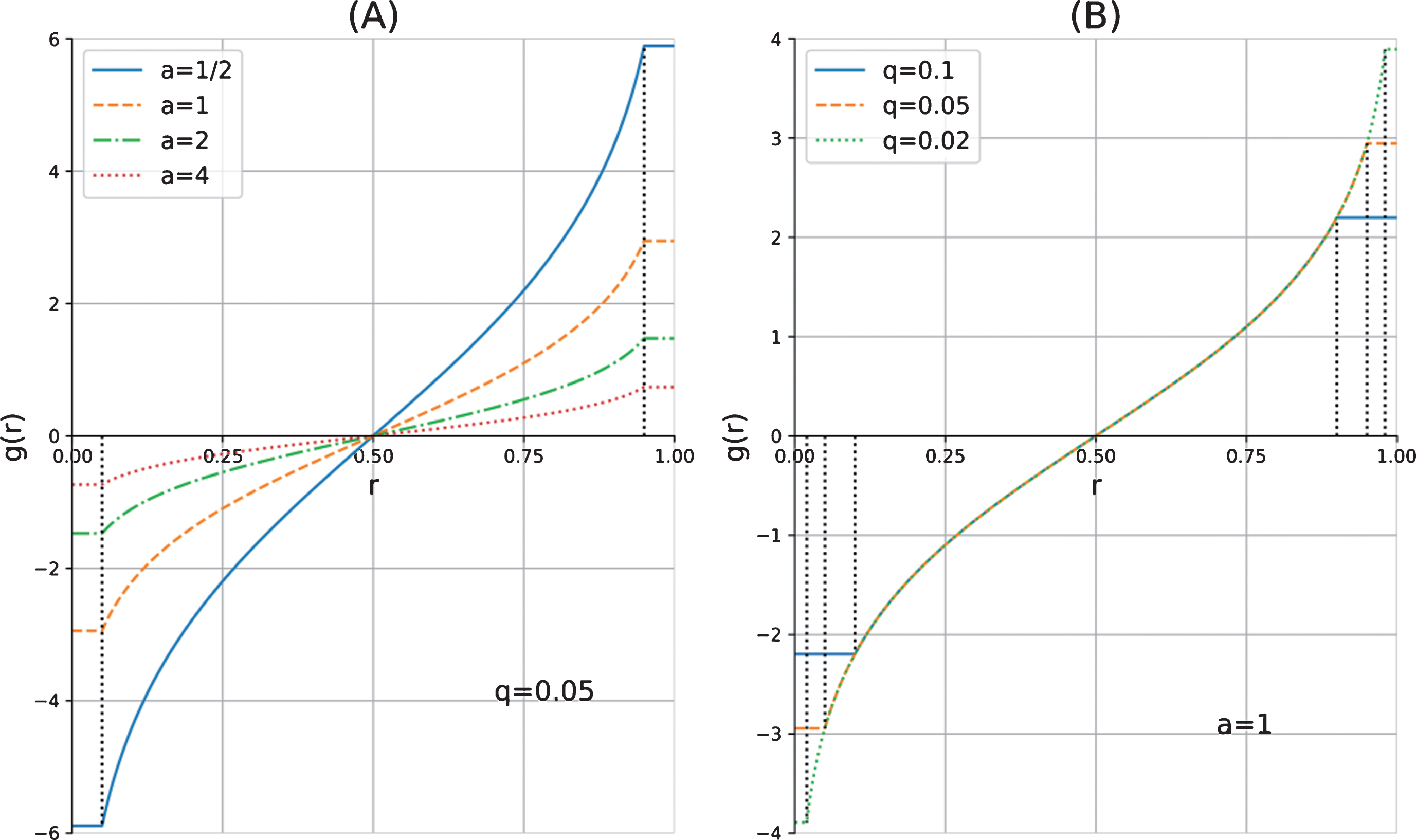
The conversion function g (r) with adjustable parameters a and q.

Figure 1 also shows the effect of different settings of parameters on the conversion function g (r). In Fig. 1 (A) we fix the parameter q = 0.05, while the parameter a is set to be 0.5, 1, 2 and 4 separately. It is clear that the smaller the parameter a, the sharper the increase of g (r) with respect to r. In Fig. 1 (A) we fix the parameter a = 1, while the parameter q is set to be 0.1, 0.05 and 0.02 separately. And the greater the parameter q, the more insensitive the DM is to the preference values, as in the DM can overlook greater deviation between the preference values 0 and q, as well as 1 - qand 1, deeming them as indifferent.

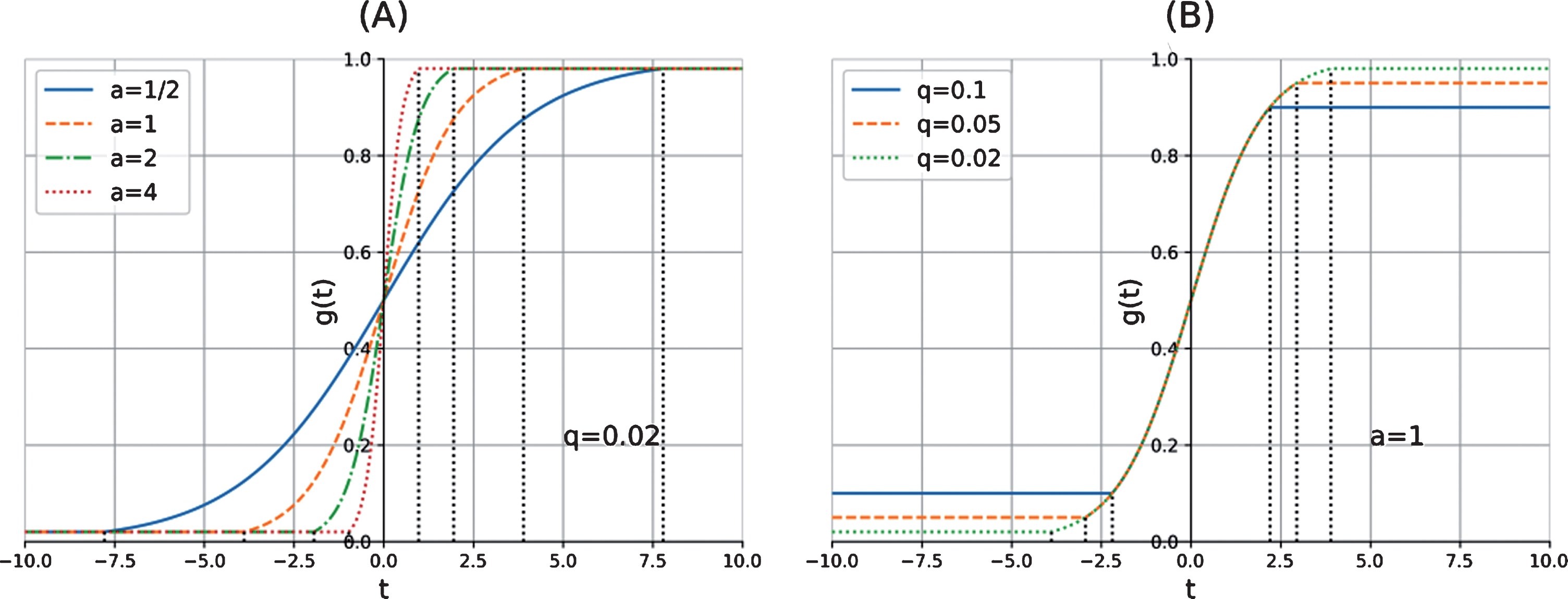
Since the fundamental purpose of constructing the Bayesian linear regression model is to estimate the unknown preference values in IFRPR, it is necessary to convert the results obtained from (- ∞ , + ∞) to [0, 1]. Like illustrated in Fig. 2 we now consider the inverse function r = g^-1 (t): $g^{- 1} (t) = {\begin{matrix} \begin{matrix} 1 / (1 + e^{aQ}), & t \leq - Q \end{matrix} \\ \begin{matrix} 1 / (1 + e^{- at}), & Q < t < - Q \end{matrix} \\ \begin{matrix} 1 / (1 + e^{- aQ}), & t \geq Q \end{matrix} \end{matrix}$ (17) where Q = (1/ - a) · ln(1 - q)/ - q.

Fig.2

The inverse conversion function g^-1 (t) with adjustable parameters a and q.

Note when t ≤ - Q, 1/ - 1 + e^aQ = q > 0; and when t ≥ Q, 1/ - 1 + e^-aQ = 1 - q < 1, therefore after converting with g^-1 (t), the results should all satisfy the requirements of fuzzy preference relations. It is worth noting that g^-1 (t) is monotonically increasing, and the closer t to 0, the sharper increase of g^-1 (t) with respect to t; meanwhile the closer t to ±Q, the slower increase of g^-1 (t) with respect to t.

This feature is actually the reason that we chose to utilize the conversion function in Equation (16), and it is desirable because we believe that with the adjustable parameters, it can model some characteristics of human perception in the decision-making process. Recall that we assume the probability distribution of the target variable t, which essentially is the converted preference value given by the experts, takes the form of Gaussian distribution. In other words, let us suppose that $t \sim N (μ, Σ)$ , then it is always true that P (t = μ - a) = P (t = μ + a), $\forall a \in ℝ$ . If we had chosen a linear conversion function, then after conversion we would also have P (r = g^-1 (μ - a)) = P (r = g^-1 (μ + a)), since the derivative of the linear function is always constant.But we believe that this may not be the case when g^-1 (μ) is very close to 0 or 1. Suppose g^-1 (μ) is very close to 1, when deciding upon a proper preference value that can reflect his or her opinions and knowledge of the alternatives, the DM may be reluctant to show strict preference for he or she would like to show that the judgement made is fair, reasonable and impartial. So as a result it is reasonable to assume that the original preference values provided by the experts are not strictly normally distributed, which means that given $a \in ℝ$ that is small enough, and we would have P (r = g^-1 (μ - a))≥ P (r = g^-1 (μ + a)). Hence it is desirable that the closer t to Q, the slower increase of g^-1 (t) with respect to t, similar argument can also be made when t approximates -Q.

3.2 The Bayesian model of estimating the unknown preference value

Now with conversion function, we can construct the general Bayesian linear regression model for the unknown preference values in IFRPR. Recall that given any IFRPR R^l (l = 1 : N), it is always true that ∀i, j = 1 : M, $r_{ij}^{(l)} + r_{ji}^{(l)} = 1$ , and $r_{ii}^{(l)} = 0.5$ . So here we only need to take into account M (M - 1)/2 preference values: ${r_{ij}^{(l)} | i, j = 1 : M, i < j}$ .

For brevity, for now we assume that only one expert e_h provided IFRPR R^h, with only one pair of preference values $r_{uv}^{(h)}$ and $r_{vu}^{(h)}$ missing, and without loss of generality, we also assume that u < v. Other circumstances will later be discussed later in subsection 3.4. By assumption, given any one of the remaining experts e_l ∈ E ∖ {e_h}, the preference relation R^l he or she provided would be complete. And after conversion with formula (16), the preference values of R^l can be rearranged into a K = M (M - 1)/2 - 1 dimensional predictor $\begin{matrix} x^{(l)} ≜ (g (r_{1, 2}^{(l)}), . . ., g (r_{1, M}^{(l)}), . . ., \\ g (r_{u, v - 1}^{(l)}), g (r_{u, v + 1}^{(l)}), . . ., g (r_{M - 1, M}^{(l)})) \\ ≜ (x_{1}^{(l)}, x_{2}^{(l)}, . . ., x_{K}^{(l)}) \end{matrix}$ (18) and a scalar target variable $t^{(l)} = g (r_{uv}^{(l)})$ .Then with these notations, the problem of estimating the missing preference value $r_{uv}^{(l)}$ is turned into a regression problem: given a data set compromising N - 1 observations X = { x ^(l)|l = 1 : N, l ≠ h}, and their corresponding target values t = {t^(l)|l = 1 : N, l ≠ h}, the goal is to predict the target value t^(h) given the new input x ^(h).

Notice that the number of observations in the data set is roughly the number of experts consulted with the GDM problem, while the number of inputs is roughly half the square of the number of alternatives. That is to say, in practical applications the under-sample problem may occur, where the number of inputs is greater than the number of samples. And to overcome this problem, the Bayesian linear regression is chosen to estimate the missing preference value because it has no need for cross validation and therefore utilizes all the samples provided. Another advantage of Bayesian linear regression is that it models the associations between the predictors and the target variable with probability distribution, which allows some degree of uncertainty for the expert with IFRPRs.

We now give an illustrative example to show the conversion process and the rearrangement of preference values.

Example 2. For the sake of simplicity, here we only take a small set of alternatives A = {a₁, a₂, a₃, a₄} and experts E = {e₁, e₂, e₃, e₄, e₅, e₆, e₇, e₈}, the IFRPRs provided by each experts are as follows: $R^{1} = [\begin{matrix} 0.50 & 0.40 & 0.65 & 0.45 \\ 0.60 & 0.50 & 0.60 & 0.35 \\ 0.35 & 0.40 & 0.50 & 0.50 \\ 0.55 & 0.65 & 0.50 & 0.50 \end{matrix}],$ $R^{2} = [\begin{matrix} 0.50 & 0.95 & 0.45 & 0.85 \\ 0.05 & 0.50 & 0.30 & 0.95 \\ 0.55 & 0.70 & 0.50 & 0.35 \\ 0.15 & 0.05 & 0.65 & 0.50 \end{matrix}],$ $R^{3} = [\begin{matrix} 0.50 & 0.40 & 0.25 & 0.30 \\ 0.60 & 0.50 & 0.45 & 0.60 \\ 0.75 & 0.55 & 0.50 & 0.40 \\ 0.70 & 0.40 & 0.60 & 0.50 \end{matrix}],$ $R^{4} = [\begin{matrix} 0.50 & 0.05 & 0.50 & 0.00 \\ 0.95 & 0.50 & 0.65 & 0.30 \\ 0.5 & 0.35 & 0.50 & 0.15 \\ 1.00 & 0.70 & 0.85 & 0.50 \end{matrix}],$ $R^{5} = [\begin{matrix} 0.50 & 0.15 & 0.60 & 0.65 \\ 0.85 & 0.50 & 0.65 & 0.65 \\ 0.40 & 0.35 & 0.50 & 0.90 \\ 0.35 & 0.35 & 0.10 & 0.50 \end{matrix}],$ $R^{6} = [\begin{matrix} 0.50 & 0.25 & 0.85 & 0.30 \\ 0.75 & 0.50 & ? & 0.15 \\ 0.15 & ? & 0.50 & 0.35 \\ 0.70 & 0.85 & 0.65 & 0.50 \end{matrix}],$ $R^{7} = [\begin{matrix} 0.50 & 0.75 & 0.20 & 0.50 \\ 0.25 & 0.50 & 0.25 & 0.60 \\ 0.80 & 0.75 & 0.50 & 0.40 \\ 0.50 & 0.40 & 0.60 & 0.50 \end{matrix}],$ $R^{8} = [\begin{matrix} 0.50 & 0.25 & 0.60 & 0.80 \\ 0.75 & 0.50 & 0.65 & 0.80 \\ 0.40 & 0.35 & 0.5 & 0.90 \\ 0.20 & 0.20 & 0.10 & 0.50 \end{matrix}] .$

Notice that the IFRPR R⁶ provided by expert e₆ is incomplete with preference values $r_{23}^{(6)}$ and $r_{32}^{(6)}$ missing. It is obvious that $r_{23}^{(6)} + r_{32}^{(6)} = 1$ according to the definition of IFRPR, so here we only need to estimate the missing preference value $r_{23}^{(6)}$ .

To start with, the range of the preference values need to be converted from [0, 1]to (- ∞ , + ∞). Here we set the parameters as a = 1 and q = 0.02, then the conversion function can be written as $g (r) = {\begin{matrix} \begin{matrix} ln q / (1 - q), & 0 \leq r \leq 0.02 \end{matrix} \\ \begin{matrix} ln r / (1 - r), & 0.02 < r < 0.98 \end{matrix} \\ \begin{matrix} ln (1 - q) / q, & 0.98 \leq r \leq 1 \end{matrix} \end{matrix}$

If we take expert e₁ for instance, the preference value $r_{12}^{(1)}$ is converted to $g (r_{12}^{(1)}) = ln [r_{12}^{(1)} / (1 - r_{12}^{(1)})]$ ≈-0.4055.

Then after conversion with g (r), the complete FRPRs provided by the other 7 experts need to be rearranged into the form of observations and target variables. For instance, the FRPRP¹ provided by expert e₁ is rearrange into a predictor x ⁽¹⁾ =(-0.4055, 0.6190, - 0.2007, - 0.6190, 0) and a scalar response variable t⁽¹⁾ = 0.4055. With similar procedure, we would obtain a training data set compromising of 7 observations { x ⁽ⁱ⁾|i = 1 : 8, i ≠ 6} and their corresponding target variables {t⁽ⁱ⁾|i = 1 : 8, i ≠ 6}, which are listed in Table 1.

Table 1

The training data set compromising of 7 observations and their corresponding target variables

i	$x_{1}^{(i)}$	$x_{2}^{(i)} .$	$x_{3}^{(i)}$	$x_{4}^{(i)}$	$x_{6}^{(i)}$	t ⁽ⁱ⁾
i = 1	–0.4055	0.6190	–0.2007	–0.6190	0	0.4055
i = 2	2.9444	–0.2007	1.7346	2.9444	–0.6190	–0.8473
i = 3	–0.4055	–1.0986	–0.8473	0.4055	–0.4055	–0.2007
i = 4	–2.9444	0	3.8918	–0.8473	–1.7346	0.6190
i = 5	–1.7346	0.4055	0.6190	0.6190	2.1972	0.6190
i = 7	1.0986	–1.3863	0	0.4055	–0.4055	–1.0986
i = 8	–1.0986	0.4055	1.3863	1.3863	2.1972	0.6190

So far, the estimation of unknown preference value has been transformed into the problem of predicting t⁽⁶⁾, given the new input predictor x ⁽⁶⁾ = (-1.0986, 1.7346, - 0.8473, - 1.7346, - 0.6190). □

Next the detailed process of Bayesian linear regression for estimating the missing preference value is described. Like in Section 2.2, let w = (w₁, . . . , w_K) ^T be the weight vector of the regression, and ɛ a zero mean Gaussian noise with precision β, we take the assumption that the target value t is generated by a deterministic linear function with additive Gaussian noise. For simplicity, here we chose the most commonly used form of basic functions, $φ_{k} (x^{(l)}) = x_{k}^{(l)}$ (k = 1 : K), then the probability distribution of t can then be written as $P (t | x, w, β) = N (t | w^{T} x, β^{- 1})$ (19)

If we assume that the converted preference values are drawn independently from the distribution (19), then we would have the likelihood function: $P (t | X, w, β) = \prod_{l = 1, l \neq h}^{N} N (t^{(l)} | w^{T} x^{(l)}, β^{- 1})$ (20)

Next we also assume a zero-mean isotropic Gaussian distribution with a single precision hyper parameter α for the prior of parameters like in Equation (5), then following the standard results in Bayesian linear regression, the posterior distribution of the parameters is as described in Equations (7), (8) and (9) where $P (w | t, X, α, β) = N (w | μ_{N}, Σ_{N})$ (21) $μ_{N} = β Σ_{N} Φ^{T} t$ (22) $Σ_{N}^{- 1} = α I + β Φ^{T} Φ$ (23) and the design matrix is $Φ = {[\begin{matrix} x_{1}^{(1)} & x_{2}^{(1)} & \dots & x_{K}^{(1)} \\ x_{1}^{(2)} & x_{2}^{(2)} & \dots & x_{K}^{(2)} \\ ⋮ & ⋮ & ⋱ & ⋮ \\ x_{1}^{(N)} & x_{2}^{(N)} & \dots & x_{K}^{(N)} \end{matrix}]}_{(N - 1) \times K}$ (24)

Now with the posterior distribution, we can make predictions for the target value t^(h). Following similar procedures like described in subsection 2.2, we can have the predictive distribution $\begin{matrix} P (t^{(h)} | t, X, x^{(h)}, α, β) \\ = N (t^{(h)} | μ_{N}^{T} x^{(h)}, σ_{N}^{2} (x^{(h)})) \end{matrix}$ (25) where $σ_{N}^{2} (x^{(h)}) = 1 / β + (x^{(h)})^{T} Σ_{N} x^{(h)}$ (26)

Example 3. (Example 2 continuance) With the training data sets listed in Table 1, we first set the hyper parameters α = β = 10^-6 by default, and train the model to fit the data sets, the result is listed below: $\begin{matrix} w = (- 0.3551, 0.5030, - 0.0966, \\ 0.1526, - 0.0561)^{T}, \\ α = 11.3633, β = 81.2127 \end{matrix}$ $\begin{matrix} Σ_{N} = (α I + β Φ^{T} Φ)^{- 1} \approx \\ [\begin{matrix} \begin{matrix} \begin{matrix} 0.0040 & - 0.0024 \end{matrix} & 0.0032 & - 0.0053 & 0.0036 \end{matrix} \\ \begin{matrix} \begin{matrix} \begin{matrix} - 0.0024 & 0.0062 \end{matrix} & - 0.0026 & 0.0042 & - 0.0037 \end{matrix} \\ \begin{matrix} \begin{matrix} 0.0032 & - 0.0026 \end{matrix} & 0.0034 & - 0.0047 & 0.0034 \end{matrix} \\ \begin{matrix} \begin{matrix} \begin{matrix} - 0.0053 & 0.0042 \end{matrix} & - 0.0047 & 0.0085 & - 0.0056 \end{matrix} \\ \begin{matrix} \begin{matrix} 0.0036 & - 0.0037 \end{matrix} & 0.0034 & - 0.0056 & 0.0049 \end{matrix} \end{matrix} \end{matrix} \end{matrix}], \end{matrix}$ $\begin{matrix} μ_{N} = β Σ_{N} Φ^{T} t \\ \approx [- 0.3998, 0.5644, - 0.1448, 0.2184, - 0.1130]^{T} . \end{matrix}$

Now given the new input x ⁽⁶⁾ = (-1.0986, 1.7346, -0.8473, - 1.7346, - 0.6190), with Equations (25) and (26), we have: $σ_{N}^{2} (x^{(6)}) = \frac{1}{β} + (x^{(6)})^{T} Σ_{N} x^{(6)} \approx 0.0332$ $μ_{N}^{T} x^{(6)} \approx 1.2321$

In other words, for the new observation x ⁽⁶⁾, the probability distribution of the corresponding target variable t⁽⁶⁾ is $P (t^{(6)} | t, X, x^{(6)}, α, β) = N (t^{(6)} | 1.2321, 0.0332) .$

3.3 Representation of the prediction results with interval-valued fuzzy reciprocal preference relation

In the subsection 3.2 above, we obtained the predictive distribution of the target variable. And to complete the IFRPRs, additional procedures must be carried out to extract information about the unknown preference values from the predictive distribution in Equation (25). The naïve approach would be taking the expectation of Equation (25) and converting it back into the range of unit interval. But since the fundamental reason that we proposed to take a probabilistic perspective in the first place is to model the uncertainty and ambiguousness of the DM, and valuable information may be lost by simply replacing the unknown value with the converted expectation, here we proposed to express the prediction result in the form of Interval-Valued Fuzzy Reciprocal Preference Relation (IVFRPR), the definition of which is given below.

Definition 4. Let Λ ([0, 1]) be the set of all closed sub-intervals of [0, 1]. An Interval-Valued Fuzzy Reciprocal Preference Relation (IVFRPR) $\tilde{R}$ on a finite set of alternatives A = {a₁, a₂, . . . , a_M} (M ≥ 2) is a fuzzy set on the product set A × A, which is characterized by a membership function $π_{\tilde{R}} : A \times A \to Λ ([0, 1])$ , with $π_{\tilde{R}} (a_{i}, a_{j}) = {\tilde{r}}_{ij} = [{\tilde{r}}_{ij}^{-},$ ${\tilde{r}}_{ij}^{+}]$ , verifying ${\tilde{r}}_{ij}^{-} + {\tilde{r}}_{ji}^{+} = {\tilde{r}}_{ij}^{+} + {\tilde{r}}_{ji}^{-} = 1, \forall i, j = 1 : M$ .

In subsection 3.2, Equations (25) and (26) show the predictive result of the target variable P (t^(h)), which takes the form of Gaussian distribution. It is well known that for Gaussian distribution $N (μ, σ^{2})$ , according to the empirical rule, the values that lies in [μ - σ, μ + σ] account for 68.27% of the whole set; while [μ - 2σ, μ + 2σ] account for 95.44%; and [μ - 3σ, μ + 3σ] account for 99.74%. Thus loosely speaking, for the predictive distribution in Equation (25), we can be 95.44% confident that the target variable will lie between the interval $[μ_{N}^{T} x^{(h)} - 2 σ_{N} (x^{(h)}), μ_{N}^{T} x^{(h)} + 2 σ_{N} (x^{(h)})]$ (27) and 99.74% confident that the target variable will lie between the interval $[μ_{N}^{T} x^{(h)} - 3 σ_{N} (x^{(h)}), μ_{N}^{T} x^{(h)} + 3 σ_{N} (x^{(h)})]$ (28)

Admittedly other confidence level ξ can also be utilized as long as it satisfies the equation P (c₁ ≤ t ≤ c₂) = ξ, where [c₁, c₂] is the corresponding interval. But it is reasonable to believe that the interval of two or three deviations away from the mean value would suffice to meet most of the practical demands.

Without loss of generality, here we assume that for the probability distribution in Equation (25) of the target variable t^(h),the chosen confidence level is ξ with corresponding confidence interval [c₁, c₂], namely P (c₁ ≤ t^(h) ≤ c₂) = ξ. Then because the conversion function g^-1 (t) in Equation (17) is monotonically increasing, so after conversion we would have $P (g^{- 1} (c_{1}) \leq r_{uv}^{(h)} \leq g^{- 1} (c_{2})) = ξ$ (29) which means that for the unknown preference value $r_{uv}^{(h)}$ , we are with confidence level ξ that it lies between the interval [g^-1 (c₁) , g^-1 (c₂)].

As aforementioned, we proposed to represent the predictive result in the form of IVFRPRs. For the unknown preference value $r_{uv}^{(h)}$ , we take the confidence interval [g^-1 (c₁) , g^-1 (c₂)] with sufficient confidence level as the prediction result, then according to the definition of the IVFRPR, we would have ${\tilde{r}}_{vu}^{(h)} = [1 - g^{- 1} (c_{2}), 1 - g^{- 1} (c_{1})]$ . Furthermore, notice that for ${\tilde{r}}_{ij} = [{\tilde{r}}_{ij}^{-}, {\tilde{r}}_{ij}^{+}]$ , when ${\tilde{r}}_{ij}^{-} = {\tilde{r}}_{ij}^{+}$ , it is reduced to crisp-valued fuzzy reciprocal preference value. So for the other known preference values that expert e_h did provide, let ${\tilde{r}}_{ij}^{(h)} = [r_{ij}^{(h)}, r_{ij}^{(h)}]$ for ∀i, j = 1 : M, then we would have a complete IVFRPR ${\tilde{R}}^{h}$ .

Example 4. (Example 2 and 3 continuance) From the results of Example 1 and 2, the probability distribution of the target variable t⁽⁶⁾ is $N (t^{(6)} | 1.2321,$ 0.0332). If we take the interval of two deviations away from the mean value as confidence interval for demonstration, then we can be 95.44% confident that the target variable t⁽⁶⁾ lies between the interval [1.1657, 1.2985]. So after conversion with Equation (17), we would be 95.44% confident that the unknown preference value $r_{23}^{(6)}$ lies between the interval [g^-1 (1.1657) , g^-1 (1.2985)] = [0.7623, 0.7856]. Then the completed IVFRPR of expert e₆ is obtained: ${\tilde{R}}^{6} = [\begin{matrix} [0.5, 0.5] & [0.25, 0.25] & [0.85, 0.85] & [0.3, 0.3] \\ [0.75, 0.75] & [0.5, 0.5] & [0.7623, 0.7856] & [0.15, 0.15] \\ [0.15, 0.15] & [0.2144, 0.2377] & [0.5, 0.5] & [0.35, 0.35] \\ [0.7, 0.7] & [0.85, 0.85] & [0.65, 0.65] & [0.5, 0.5] \end{matrix}] .$

3.4 Preprocessing of the preference values

In subsection 3.2, we assumed that only one expert in the group provided IFRPR, and with only one pair of preference values unknown. Unfortunately in practical applications, there may be much more complex circumstances. In this subsection, the preprocessing of the preference values is utilized to address these kinds of problems, which we believe should fall into three categories, or their combinations:

Only one expert provided IFRPR, but with more than one pair of preference values unknown.For simplicity, suppose expert e_h provided IFRPR R^h with two pairs of preference values ${r_{u_{1}, v_{1}}^{(h)}, r_{v_{1}, u_{1}}^{(h)}, r_{u_{2}, v_{2}}^{(h)}, r_{v_{2}, u_{2}}^{(h)}}$ missing. Then the estimation of the unknown values should be made one pair at each time. Specifically, the preference values of expert e_h can be rearranged into a M (M - 1) -2 dimensional predictor with two target values $r_{u_{1}, v_{1}}^{(h)}$ and $r_{u_{2}, v_{2}}^{(h)}$ . The preference values of the complete FRPR should also be rearrange in similar manners, with predictor $x^{(l)} ≜ (r_{1, 2}^{(l)}, . . ., r_{u_{1}, v_{1} - 1}^{(l)}, r_{u_{1}, v_{1} + 1}^{(l)}, . . ., r_{u_{2}, v_{2} - 1}^{(l)}, r_{u_{2}, v_{2} + 1}^{(l)},$ $. . ., r_{M - 1, M}^{(l)})$ and target variable vector $t^{(l)} = (t_{1}^{(l)}, t_{2}^{(l)})^{T}$ $= (r_{u_{1}, v_{1}}^{(l)}, r_{u_{2}, v_{2}}^{(l)})^{T}$ . Then the estimation of the unknown preference values is transformed into a multi-output regression problem, which can be solved following similar procedures described in subsection 3.2 with slight modification on the targetvariable.

More than one expert provided IFRPR, but with only one same pair of preference values missing. Suppose experts e_{h
₁} and e_{h
₂} provided IFRPRs R^{h
₁} and R^{h
₂}, but with the same pair of preference values $r_{uv}^{(h_{l})} (l = 1, 2)$ and $r_{vu}^{(h_{l})} (l = 1, 2)$ missing. This problem can be dealt with by making estimation for two experts separately using the same model constructed in subsection 3.1, only with a slightly smaller training data set X = { x ^(l)|l = 1 : N, l ≠ h₁, h₂} compromising N - 2 observations.

More than one expert provided IFRPRs, but with different pairs of preference values missing. Without loss of generality, we assume that expert e_{h
₁} and e_{h
₂} both provided IFRPRs, but R^{h
₁} is incomplete with $r_{u_{1} v_{1}}^{(h_{1})}$ and $r_{v_{1} u_{1}}^{(h_{1})}$ unknown, while R^{h
₂} is incomplete with $r_{u_{2} v_{2}}^{(h_{2})}$ and $r_{v_{2} u_{2}}^{(h_{2})}$ unknown. We first set the target variable to be t = r_{u
₁
v
₁}and train the model with data sets X = { x ^(l)|l = 1 : N, l ≠ h₁}. Then the problem arises where sample x ^(h₂) is incomplete with preference value $r_{u_{2} v_{2}}^{(h_{2})}$ missing. Here we could temporarily replace the unknown preference value $r_{u_{2} v_{2}}^{(h_{2})}$ with the mean of the corresponding preference values provided by other experts, i.e. $r_{u_{2} v_{2}}^{(h_{2})} =$ $(1 / N - 2) \cdot Σ_{l = 1, l \neq h_{1}, h_{2}}^{N} r_{u_{2} v_{2}}^{(l)}$ . Then the Bayesian model constructed in subsection 3.1 can be utilized to estimate the missing preference value $r_{u_{1} v_{1}}^{(h_{1})}$ . Similarly, next we could set the target variable to be t = r_{u
₂
v
₂} and make estimation for the unknown preference value $r_{u_{2} v_{2}}^{(h_{2})}$ .

4 Consensus reaching process

Simply put, the objective of GDM can be described as choosing the best alternative or alternatives from the set of feasible ones, on the basis of the experts’ preferences and opinions. And in order to do that, a selection process must be carried out, which usually involves two stages: the aggregation of the individual opinions provided by the experts, and the exploitation of the collective opinion of the group [19]. But some expert may be reluctant to accept the final decision result if he or she felt that his or her opinion has been neglected or not well-reflected. So it would be preferable to reach the state of consensus before entering the phase of exploitation.

But in reality, a group of experts seldom agree with each other completely, and it is nearly impossible to reach a unanimous decision due to the experts’ divergent backgrounds and possible conflict of interests. So instead of asking the experts to reach a full agreement, a softer type of consensus is proposed, where some consensus indices are defined to measure the degree of agreement among the experts. With these consensus measurements, the experts are asked to revise and modify their preferences step by step until they reach a sufficient consensus degree. A detailed demonstration of the entire CRP with IFRPRs is shown inFig. 3.

Fig.3

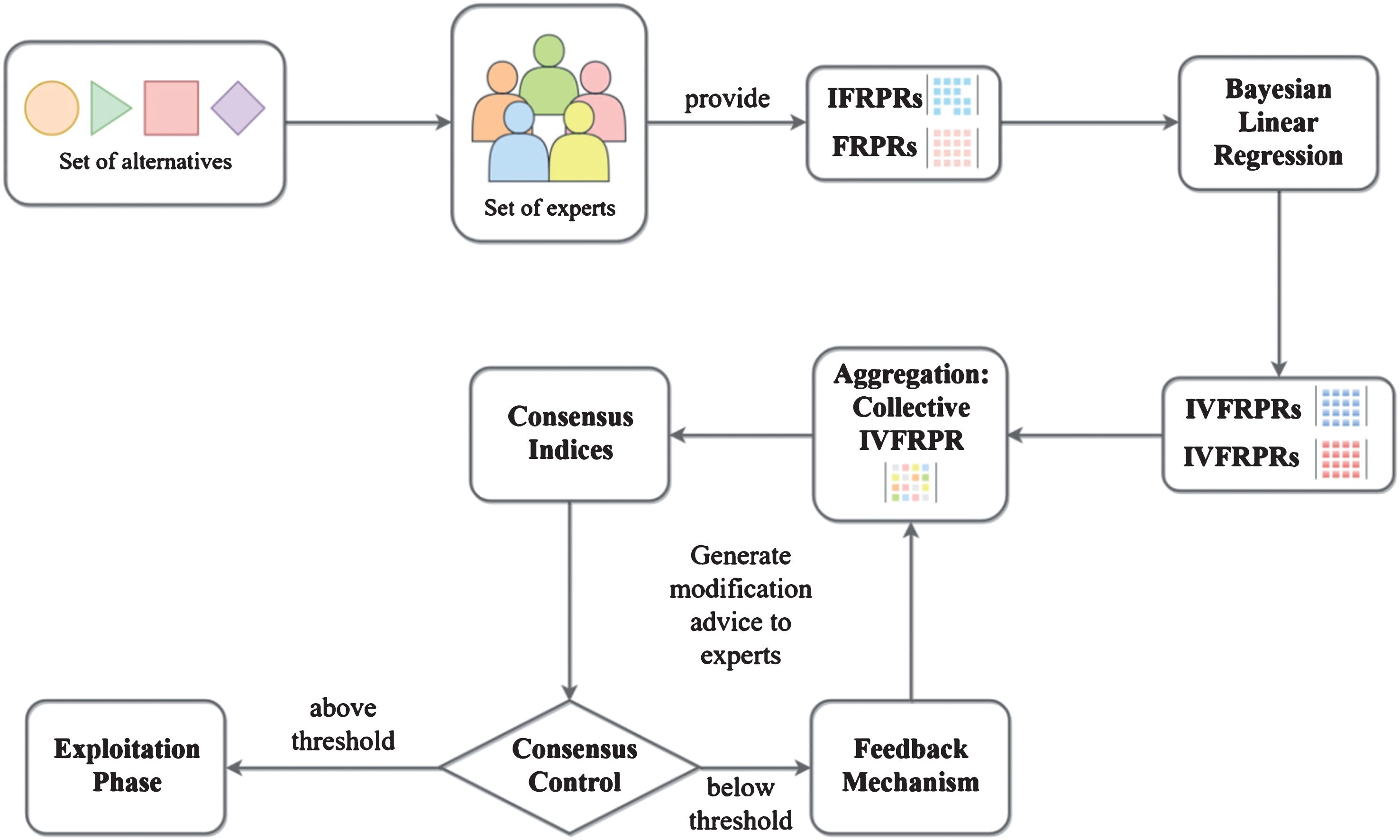
CRP in GDM with IFRPRs using Bayesian linear regression.

As illustrated in Fig. 3, the CRP with IFRPRs consists of 7 steps:

Step 1. The experts express or verbalize his or her preference of the alternatives in the form of FRPRs or IFRPRs;

Step 2. The unknown preference value in IFRPR is estimated through Bayesian linear regression and expressed in the form of probability distribution;

Step 3. The preference information of the experts is transformed into the form of IVFRPRs;

Step 4. The experts’ individual IVFRPRs are aggregated into a collective IVFRPR;

Step 5. The consensus indices of each expert to the group are computed on three levels: on pairs of alternatives, on alternatives and on preference relations;

Step 6. If the consensus indices are above the threshold, go to Step 7; otherwise the experts with insufficient consensus indices are identified, and revision advice is generated accordingly for these experts. After revision, go to Step 4;

Step 7. The selection process is carried out to choose the best alternative or alternatives as the solution to the GDM problem.

The first three steps have already been covered in Section 3,the more detailed description of Step 4 to 7 would be the focus of this section.

4.1 Consensus indices

For Step 4, we first need to aggregate each expert’s opinion ${\tilde{R}}^{h}$ into a collective one ${\tilde{R}}^{*}$ for further utilization.Given two interval-valued numbers ${\tilde{r}}_{1} = [{\tilde{r}}_{1}^{-}, {\tilde{r}}_{1}^{+}]$ and ${\tilde{r}}_{2} = [{\tilde{r}}_{2}^{-}, {\tilde{r}}_{2}^{+}]$ , some of their arithmetic operators [38] are defined as follows:

${\tilde{r}}_{1} \oplus {\tilde{r}}_{2} = [{\tilde{r}}_{1}^{-} + {\tilde{r}}_{2}^{-}, {\tilde{r}}_{1}^{+} + {\tilde{r}}_{2}^{+}]$ ;

${\tilde{r}}_{1} \otimes {\tilde{r}}_{2} = [min {{\tilde{r}}_{1}^{-} {\tilde{r}}_{2}^{-}, {\tilde{r}}_{1}^{-} {\tilde{r}}_{2}^{+}, {\tilde{r}}_{1}^{+} {\tilde{r}}_{2}^{-}, {\tilde{r}}_{1}^{+} {\tilde{r}}_{2}^{+}},$ $max {{\tilde{r}}_{1}^{-} {\tilde{r}}_{2}^{-}, {\tilde{r}}_{1}^{-} {\tilde{r}}_{2}^{+}, {\tilde{r}}_{1}^{+} {\tilde{r}}_{2}^{-}, {\tilde{r}}_{1}^{+} {\tilde{r}}_{2}^{+}}]$ ;

${\tilde{r}}_{1} / {\tilde{r}}_{2} = [{\tilde{r}}_{1}^{-}, {\tilde{r}}_{1}^{+}] \otimes [\frac{1}{{\tilde{r}}_{2}^{+}}, \frac{1}{{\tilde{r}}_{2}^{-}}]$ ;

$ω {\tilde{r}}_{1} = [ω {\tilde{r}}_{1}^{-}, ω {\tilde{r}}_{1}^{+}]$

Now with these operators we can have the weighted average operator for IVFRPRs.

Definition 5. [7] Suppose ω = (ω₁, . . . , ω_N) ^T is the weight vector with the condition that $\sum_{h = 1}^{N} ω_{h} = 1$ , Θ is the set of all IVFRPRs, the weighted average operator WA_ω : Θ^N → Θ is defined as: $\begin{matrix} {WA}_{ω} ({\tilde{R}}^{1}, . . ., {\tilde{R}}^{N}) = \oplus_{h = 1}^{N} ω_{h} {\tilde{R}}^{h} \\ = {([\sum_{h = 1}^{N} ω_{h} {\tilde{r}}_{ij}^{h -}, \sum_{h = 1}^{N} ω_{h} {\tilde{r}}_{ij}^{h +}])}_{M \times M} \end{matrix}$ (30)

Then the collective IVFRPR of the group can be obtained: ${\tilde{R}}^{*} = {WA}_{ω} ({\tilde{R}}^{1}, . . ., {\tilde{R}}^{N})$ , where ω = (ω₁, . . . , ω_N) ^T denotes the normalized weights of each individual expert. The experts’ weights can be derived through analysis of the experts’ social network, or directly asking experts to provide their trust/distrust opinions of each other [37]. Here we assume that the weight vector ω was designated beforehand.

Now we have the collective IVFRPR of the group, next in Step 5 the consensus indices of each expert e_h can be defined on three levels: pairs of alternatives, alternatives and preference relations[38].

Definition 6. (On pairs of alternatives) The consensus index CP of an expert e_h to the group of experts on the preference of alternative a_i over a_j is defined as: ${CP}_{ij}^{h} = 1 - \frac{1}{2} (| {\tilde{r}}_{ij}^{h -} - {\tilde{r}}_{ij}^{* -} | + | {\tilde{r}}_{ij}^{h +} - {\tilde{r}}_{ij}^{* +} |)$ (31)

Definition 7. (On alternatives) The consensus index CA of an expert e_h to the group of experts on the preference of alternative a_i to the rest of the alternatives is defined as: ${CA}_{i}^{h} = \frac{1}{M - 1} \sum_{j = 1, j \neq i}^{M} {CP}_{ij}^{h}$ (32)

Definition 8. (On preference relations) The consensus index CR of an expert e_h to the group of experts on the preference relation is defined as: ${CR}^{h} = \frac{1}{M} \sum_{i = 1}^{M} {CA}_{i}^{h}$ (33)

Notice that the closer the expert’s preference is to the group, the bigger the consensus indices. In the rare case that ${\tilde{R}}^{h} = {\tilde{R}}^{*}$ , for consensus index on the pair of alternatives, we have ${CP}_{ij}^{h} = 1$ for ∀i, j = 1 : M; for consensus index on the alternatives, ${CA}_{i}^{h} = 1$ for ∀i = 1 : M; for consensus index on the preference relation, CR^h = 1.

4.2 Consensus control and feedback mechanism

Usually in the CRP, to help the experts to reach sufficient consensus level within an acceptable time frame, a moderator is often present [19]. A moderator’s first responsibility is to compute the consensus levels of each expert according to the IVFRPRs they provided, and to deem if sufficient consensus level has been reached. Suppose γ is the designated consensus threshold, it is deemed as acceptable consensus within the group if for every expert in E = {e_h|h = 1 : N}, we have CR^h ≥ γ. If so, the CRP is terminated and the exploitation of the collective IVFRPRs of the group is carried out; if not, the moderator then needs to identify those experts with insufficient consensus levels, which can also be described on three levels: on preference relation, on alternatives and on pairs of alternatives [38].

The experts with insufficient consensus index CR on the preference relation are identified: $EXPCH = {h | {CR}^{h} < γ} .$

For those experts in EXPCH, the alternatives on which their consensus index is below the threshold are identified: $ALT = {(h, i) | h \in EXPCH \land {CA}_{i}^{h} < γ} .$

For those alternatives in ALT, the pairs of alternatives whose preference value needs revision are identified: $APS = {(h, i, j) | (h, i) \in ALT \land {CP}_{ij}^{h} < γ \land i < j} .$

The moderator will then supply this information as feedback to the experts with insufficient consensus indices. To accelerate the CRP, suppose (h, i, j) ∈ APS, the moderator will also generate revision advices for expert e_h: “The consensus index of your preference of alternative a_i over a_i is ${CP}_{ij}^{h}$ , which is below the designated threshold γ. It is advisable to revise it to a value closer to ${\tilde{r}}_{ij}^{*}$ .” and the experts are expected to revise his or her preferences accordingly. The revised IVFRPRs are then aggregated again to form the new collective IVFRPR, and this process is repeated round by round until sufficient consensus level isreached.

4.3 Exploitation phase

Up till now, the first 6 steps of the CRP are completed, we now have the collective IVFRPR ${\tilde{R}}^{*}$ with sufficient consensus level, Step 7 focuses on the exploitation of said ${\tilde{R}}^{*}$ .

With the arithmetic operators of interval numbers described in subsection 4.1, we can calculate the average preference degree ρ_i [7] of alternative a_iover the rest of the alternatives as: $ρ_{i} = \frac{\oplus_{j = 1}^{M} {\tilde{r}}_{ij}^{*}}{\oplus_{i = 1}^{M} \oplus_{j = 1}^{M} {\tilde{r}}_{ij}^{*}}, \forall i = 1 : M$ (34)

To compare two interval numbers, in [43] Xu defined the possibility degree of ρ_i ≥ ρ_j as:∀i, j = 1 : M $\begin{matrix} d_{ij} ≜ d (ρ_{i} \geq ρ_{j}) \\ = min {max (\frac{ρ_{i}^{+} - ρ_{j}^{-}}{ρ_{i}^{+} - ρ_{j}^{-} + ρ_{j}^{+} - ρ_{i}^{-}}, 0), 1} \end{matrix}$ (35)

Then the complementary matrix D = (d_ij) _M×M is constructed, and it is easy to see that d_ij > 0, d_ij + d_ji = 1, d_ii = 0, ∀ i, j = 1 : M.

Finally in [7], the author defined the ranking value RV (a_i) of alternative a_i as: $RV (a_{i}) = \frac{2}{M^{2}} \sum_{j = 1}^{M} d_{ij}, \forall i = 1 : M$ (36)

Then the alternative or alternatives with the highest ranking value would be selected as the solution to the GDM problem, and Step 7 of the CRP is completed at last.

5 Case study

To demonstrate the entire procedure of CRP with IFRPRs based on Bayesian linear regression, here we provide a case study about possible application of our proposed model in project performanceevaluations.

Project performance evaluations is a method by which the design, implementation and performance of a project is documented and evaluated. Since a project usually takes up a relatively long period of time, varying from months to years depending on the objectives and nature of the project itself, it is a common practice to divide the project into several stages or tranches. Then at the end of each stage, a performance evaluation process is often carried out, to determine if the project has been satisfactorily accomplished on schedule. What’s more, the results from the performance evaluations can then be used to make comparisons with other projects of similar natures, and serve as the bases of assigning rewards to those who have achieved great accomplishments, or providing improvement advices to those who has fallen behindschedule.

To ensure the impartiality and rationality of the performance evaluation process, usually a group of experts are consulted. So in other words the performance evaluation process can be described as a group of experts gathered to obtain a fair ranking of a set of projects, hence a GDM problem. And since the human judgement is inherently imprecise and ambiguous, it is more reasonable to formalize the project evaluation process as a fuzzy GDM problem. Suppose there are 12 experts, denoted as E = {e_n|n = 1 : 12} who are gathered to evaluate and rank the performance of four projects with similar natures, denoted as A = {a_i|i = 1 : 4}. Next our proposed method is carried out in detailedprocedures.

Step 1. All experts are instructed to provide his or her opinions through pairwise comparison between two alternatives and verbalize his or her preferences with a crisp number in the unit interval [0, 1]. And the IFRPRs of all 12 experts areobtained: $R^{1} = [\begin{matrix} 0.50 & 0.15 & 0.85 & 0.30 \\ 0.85 & 0.50 & 0.80 & 0.10 \\ 0.15 & 0.20 & 0.50 & 0.45 \\ 0.70 & 0.90 & 0.55 & 0.50 \end{matrix}],$ $R^{2} = [\begin{matrix} 0.50 & 0.75 & 0.80 & 0.80 \\ 0.25 & 0.50 & 0.70 & 0.65 \\ 0.20 & 0.30 & 0.50 & ? \\ 0.20 & 0.35 & ? & 0.50 \end{matrix}],$ $R^{3} = [\begin{matrix} 0.50 & 0.35 & 0.35 & 0.30 \\ 0.65 & 0.50 & 0.45 & 0.40 \\ 0.65 & 0.55 & 0.50 & 0.45 \\ 0.70 & 0.60 & 0.55 & 0.50 \end{matrix}],$ $R^{4} = [\begin{matrix} 0.50 & 0.70 & 0.55 & 0.40 \\ 0.30 & 0.50 & 0.40 & 0.25 \\ 0.45 & 0.60 & 0.50 & 0.35 \\ 0.60 & 0.75 & 0.65 & 0.50 \end{matrix}],$ $R^{5} = [\begin{matrix} 0.50 & 0.75 & 0.05 & 0.60 \\ 0.25 & 0.50 & 0.40 & 0.95 \\ 0.95 & 0.60 & 0.50 & 0.50 \\ 0.40 & 0.05 & 0.50 & 0.50 \end{matrix}],$ $R^{6} = [\begin{matrix} 0.50 & 0.90 & 0.50 & 1.00 \\ 0.10 & 0.50 & 0.55 & 0.65 \\ 0.50 & 0.45 & 0.50 & 0.95 \\ 0.00 & 0.35 & 0.05 & 0.50 \end{matrix}],$ $R^{7} = [\begin{matrix} 0.50 & 0.80 & 0.65 & 0.65 \\ 0.20 & 0.50 & ? & 0.35 \\ 0.35 & ? & 0.50 & 0.50 \\ 0.35 & 0.65 & 0.50 & 0.50 \end{matrix}],$ $R^{8} = [\begin{matrix} 0.50 & 0.95 & 0.75 & 0.60 \\ 0.05 & 0.50 & 0.30 & 0.35 \\ 0.25 & 0.70 & 0.50 & 0.20 \\ 0.40 & 0.65 & 0.80 & 0.50 \end{matrix}],$ $R^{9} = [\begin{matrix} 0.50 & 0.55 & 0.85 & 0.55 \\ 0.45 & 0.50 & 0.50 & 0.55 \\ 0.15 & 0.50 & 0.50 & 0.15 \\ 0.45 & 0.45 & 0.85 & 0.50 \end{matrix}],$ $R^{10} = [\begin{matrix} 0.50 & 0.50 & 0.50 & 0.40 \\ 0.50 & 0.50 & 0.60 & 0.60 \\ 0.50 & 0.40 & 0.50 & 0.20 \\ 0.60 & 0.40 & 0.80 & 0.50 \end{matrix}],$ $R^{11} = [\begin{matrix} 0.50 & 0.40 & 0.25 & 0.30 \\ 0.60 & 0.50 & 0.40 & 0.40 \\ 0.75 & 0.60 & 0.50 & 0.50 \\ 0.70 & 0.60 & 0.50 & 0.50 \end{matrix}],$ $R^{12} = [\begin{matrix} 0.50 & 0.10 & 0.45 & 0.10 \\ 0.90 & 0.50 & 0.70 & 0.40 \\ 0.55 & 0.30 & 0.50 & 0.30 \\ 0.90 & 0.60 & 0.70 & 0.50 \end{matrix}]$

Step 2. Notice that two out of twelve experts provided IFRPRs, more specifically, expert e₂provided IFRPR with $r_{34}^{(2)}$ and $r_{43}^{(2)}$ unknown; and expert e₇ provided IFRPR with $r_{23}^{(7)}$ and $r_{32}^{(7)}$ unknown, which falls into the third category described in subsection 3.2, namely more than one expert provided IFRPR and with different pairs of preference values unknown.

We first estimate the unknown preference value of R² through Bayesian linear regression. For the time being we need to temporarily replace the unknown preference values $r_{23}^{(7)}$ and $r_{32}^{(7)}$ in R⁷ so that the rest of the information in IFRPR provided by expert e₇ can be admissible. Here we temporarily replace $r_{23}^{(7)}$ with the mean $(1 / 10) \cdot Σ_{n = 1, n \neq 2, 7}^{12} r_{23}^{(n)} = 0.51$ . Then we set the target variable as $r_{34}^{(n)}$ , and convert the preference values with function $g (r) = {\begin{matrix} \begin{matrix} - 3.8918, & 0 \leq r \leq 0.02 \end{matrix} \\ \begin{matrix} ln r / (1 - r), & 0.02 < r < 0.98 \end{matrix} \\ \begin{matrix} 3.8918, & 0.98 \leq r \leq 1 \end{matrix} \end{matrix},$ and rearrange them into the form of observations with corresponding target values. For instance, the IFRPR provided by expert e₇ is rearranged as x ⁽⁷⁾ = [1.3863, 0.6190, 0.6190, 0.0400, - 0.6190] ^T and target variable t⁽⁷⁾ = 0. Similar procedures would be carried out for the rest of the experts, and the training data set compromising 11 observations would be obtained, the results are shown in Table 2.

Table 2
The training data set compromising of 11 observations and their corresponding target variables

i $x_{1}^{(i)}$ $x_{2}^{(i)}$ $x_{3}^{(i)}$ $x_{4}^{(i)}$ $x_{6}^{(i)}$ t ⁽ⁱ⁾

i = 1 –1.7346 1.7346 –0.8473 1.3863 –2.1972 –0.2007

i = 3 –0.6190 –0.6190 –0.8473 –0.2007 –0.4055 –0.2007

i = 4 0.8473 0.2007 –0.4055 –0.4055 –1.0986 –0.6190

i = 5 1.0986 –2.9444 0.4055 –0.4055 2.9444 0

i = 6 2.1972 0 3.8918 0.2007 0.6190 2.9444

i = 7 1.3863 0.6190 0.6190 –1.0986 –0.6190 0

i = 8 2.9444 1.0986 0.4055 –0.8473 –0.6190 –1.3863

i = 9 0.2007 1.7346 0.2007 0 0.2007 –1.7346

i = 10 0 0 –0.4055 0.4055 0.4055 –1.3863

i = 11 –0.4055 –1.0986 –0.8473 –0.4055 –0.4055 0

i = 12 –2.1972 –0.2007 –2.1972 0.8473 –0.4055 –0.8473

i	$x_{1}^{(i)}$	$x_{2}^{(i)}$	$x_{3}^{(i)}$	$x_{4}^{(i)}$	$x_{6}^{(i)}$	t ⁽ⁱ⁾
i = 1	–1.7346	1.7346	–0.8473	1.3863	–2.1972	–0.2007
i = 3	–0.6190	–0.6190	–0.8473	–0.2007	–0.4055	–0.2007
i = 4	0.8473	0.2007	–0.4055	–0.4055	–1.0986	–0.6190
i = 5	1.0986	–2.9444	0.4055	–0.4055	2.9444	0
i = 6	2.1972	0	3.8918	0.2007	0.6190	2.9444
i = 7	1.3863	0.6190	0.6190	–1.0986	–0.6190	0
i = 8	2.9444	1.0986	0.4055	–0.8473	–0.6190	–1.3863
i = 9	0.2007	1.7346	0.2007	0	0.2007	–1.7346
i = 10	0	0	–0.4055	0.4055	0.4055	–1.3863
i = 11	–0.4055	–1.0986	–0.8473	–0.4055	–0.4055	0
i = 12	–2.1972	–0.2007	–2.1972	0.8473	–0.4055	–0.8473

Next we set the parameters α = β = 10^-6 by default, and train the Bayesian linear regression model to fit the data set, the result is as follows: $\begin{matrix} w = (- 0.3380, - 0.8142, 1.0785, \\ 0.2429, - 0.7086)^{T}, \\ α = 1.8965, β = 13.1122, \end{matrix}$ $\begin{matrix} Σ_{N} = {(α I + β Φ^{T} Φ)}^{- 1} \approx \\ [\begin{matrix} \begin{matrix} \begin{matrix} 0.0147 & - 0.0031 \end{matrix} & - 0.0092 & 0.0207 & - 0.0002 \end{matrix} \\ \begin{matrix} \begin{matrix} \begin{matrix} - 0.0031 & 0.0118 \end{matrix} & - 0.0011 & - 0.0073 & 0.0092 \end{matrix} \\ \begin{matrix} \begin{matrix} - 0.0092 & - 0.0011 \end{matrix} & 0.0103 & - 0.0112 & - 0.0037 \end{matrix} \\ \begin{matrix} \begin{matrix} \begin{matrix} 0.0207 & - 0.0073 \end{matrix} & - 0.0112 & 0.0510 & 0.0009 \end{matrix} \\ \begin{matrix} \begin{matrix} - 0.0002 & 0.0092 \end{matrix} & - 0.0037 & - 0.0009 & 0.0132 \end{matrix} \end{matrix} \end{matrix} \end{matrix}], \end{matrix}$

$\begin{matrix} μ_{N} = β Σ_{N} Φ^{T} t \\ \approx [- 0.5749, - 0.7271, 1.2074, - 0.1258, - 0.6504]^{T} . \end{matrix}$

Now given the new input x ⁽²⁾ = (1.0986, 1.3863, 1.3863, 0.8473, 0.6190), with Equations (25) and (26) we have: $σ_{N}^{2} (x^{(2)}) = \frac{1}{β} + (x^{(2)})^{T} Σ_{N} x^{(2)} \approx 0.1417,$ $μ_{N}^{T} x^{(2)} \approx - 0.4750 .$

In other words, for the new observation x ⁽²⁾, the probability distribution of the corresponding target variable t⁽²⁾ is $P (t^{(2)} | t, X, x^{(2)}, α, β) = N (t^{(2)} | - 0.4750, 0.1417) .$

Similarly, a Bayesian linear regression model can also be constructed for expert e₇ with target variable set to be $\hat{t} = r_{23}^{(n)}$ and the unknown preference value of expert e₂ temporarily replaced as $r_{34}^{(2)} =$ $(1 / 10) \cdot Σ_{n = 1, n \neq 2, 7}^{12} r_{34}^{(n)} = 0.405$ , then the estimation result is given below in the form of probability distribution: $P ({\hat{t}}^{(7)} | \hat{t}, \hat{X}, {\hat{x}}^{(7)}, \hat{α}, \hat{β}) = N ({\hat{t}}^{(7)} | - 0.2919, 0.1665)$

Step 3. It is well known that for Gaussian distribution that the values within two standard deviations away from the mean account for 95.44% of the total data set. Therefore with the probability distribution of the target variable t⁽²⁾ obtained in Step 2, we are 95.44% confident that t⁽²⁾ lies between the interval [-0.7584, - 0.1916], similarly we can also be 95.44% confident that ${\hat{t}}^{(7)}$ lies between the interval [-0.6249, 0.0411]. Then to fit the basic requirement of IVFRPR, the inverse function of t = g (r) is utilized where $g^{- 1} (t) = {\begin{matrix} \begin{matrix} 0, & t = - 3.8918 \end{matrix} \\ \begin{matrix} 1 / (1 + e^{- t}), & 3.8918 < t < - 3.8918 \end{matrix} \\ \begin{matrix} 1, & t = 3.8918 \end{matrix} \end{matrix}$

And for the unknown preference $r_{34}^{(2)}$ of expert e₂, we have confidence interval [0.3190, 0.4522] with confidence level 95.44%, then by the definition of IVFRPR, we also have ${\tilde{r}}_{34}^{(2)} = [0.5478, 0.6810]$ . So now the completed IVFRPR of expert e₂ is obtained. And similarly the completed IVFRPR of expert e₇ is also obtained, the results ${\tilde{R}}^{2}$ and ${\tilde{R}}^{7}$ are shown below.

For the rest of the experts, let ${\tilde{r}}_{ij}^{(n)} = [r_{ij}^{(n)}, r_{ij}^{(n)}],$ ∀i, j = 1 : 4, n = 1 : 12, n ≠ 2, 7, then their FRPRs are also transformed into IVFRPRs.

Step 4. With IVFRPRs of 12 experts all completed, next we aggregate the individual IVFRPRs into a collective one using Equation (30) with experts’ weights all set to be equal, namely ω = (1/12, . . . , 1/12) ^T, the result ${\tilde{R}}^{*}$ is shown below. ${\tilde{R}}^{2} = [\begin{matrix} [0.5, 0.5] & [0.75, 0.75] & [0.8, 0.8] & [0.8, 0.8] \\ [0.25, 0.25] & [0.5, 0.5] & [0.7, 0.7] & [0.65, 0.65] \\ [0.2, 0.2] & [0.3, 0.3] & [0.5, 0.5] & [0.3190, 0.4522] \\ [0.2, 0.2] & [0.35, 0.35] & [0.5478, 0.6810] & [0.5, 0.5] \end{matrix}] .$ ${\tilde{R}}^{7} = [\begin{matrix} [0.5, 0.5] & [0.8, 0.8] & [0.65, 0.65] & [0.65, 0.65] \\ [0.2, 0.2] & [0.5, 0.5] & [0.3487, 0.5103] & [0.35, 0.35] \\ [0.35, 0.35] & [0.4897, 0.6513] & [0.5, 0.5] & [0.5, 0.5] \\ [0.35, 0.35] & [0.65, 0.65] & [0.5, 0.5] & [0.5, 0.5] \end{matrix}] .$ $\begin{matrix} {\tilde{R}}^{*} = {WA}_{ω} ({\tilde{R}}^{1}, . . ., {\tilde{R}}^{12}) = \oplus_{h = 1}^{12} ω_{h} {\tilde{R}}^{h} \approx \\ [\begin{matrix} [0.5, 0.5] & [0.575, 0.575] & [0.5458, 0.5458] & [0.5, 0.5] \\ [0.425, 0.425] & [0.5, 0.5] & [0.5124, 0.5259] & [0.4708, 0.4708] \\ [0.4542, 0.4542] & [0.4741, 0.4876] & [0.5, 0.5] & [0.4058, 0.4169] \\ [0.5, 0.5] & [0.5292, 0.5292] & [0.5831, 0.5942] & [0.5, 0.5] \end{matrix}] \end{matrix}$

Step 5. Now we can calculate the consensus indices of each expert on three levels via Equations (31), (32) and (33), take expert e₂ for example, the consensus indices on the pairs of alternatives are shown as below: $\begin{matrix} {CP}_{12}^{2} = 0.825, {CP}_{13}^{2} = 0.7458, {CP}_{14}^{2} = 0.7, \\ {CP}_{23}^{2} = 0.8191, {CP}_{24}^{2} = 0.8208, {CP}_{34}^{2} = 0.9390 . \end{matrix}$

For the sake of simplicity, here we only listed the consensus indices on pairs of alternatives where i < j, because it is easy to see that ${CP}_{ij}^{h} = {CP}_{ji}^{h}$ . Then the consensus indices on alternatives are also obtained where $\begin{matrix} {CA}_{1}^{2} = 0.7569, {CA}_{2}^{2} = 0.8217, \\ {CA}_{3}^{2} = 0.8346, {CA}_{4}^{2} = 0.8199 . \end{matrix}$

Finally, the consensus index of expert e₂ on preference relation is acquired: ${CR}^{2} = 0.8083 .$

Similarly, the consensus indices of other experts are calculated, the result of which is listed below: $\begin{matrix} {CR}^{1} = 0 . 7301, {CR}^{2} = 0.8083, {CR}^{3} = 0.8668, \\ {CR}^{4} = 0.8949, {CR}^{5} = 0.7570, {CR}^{6} = 0.7301, \\ {CR}^{7} = 0 . 8703, {CR}^{8} = 0.7949, {CR}^{9} = 0.8769, \\ {CR}^{10} = 0.8930, {CR}^{11} = 0.8418, {CR}^{12} = 0.7777 . \end{matrix}$

Step 6. If we set the consensus threshold at γ = 0.8, then it is clear that experts e₂, e₃, e₄, e₇, e₉, e₁₀, e₁₁ reached this threshold while experts e₁, e₅, e₆, e₈, e₁₂ failed to do so, thus EXPCH = {1, 5, 6, 8, 12}. The CRP continues and now we need to generate revision advice for those experts with insufficient consensus indices. We take expert e₁₂ as an example, first we identify on which alternative is expert e₁₂ below the consensus threshold, it is easy to see that ${CA}_{1}^{12}, {CA}_{2}^{12} < γ$ , therefore we have (12, 1) , (12, 2) ∈ALT. More specifically, we identify on which pair of alternative is expert e₁₂ divergent from the group, from Step 5 we have ${CP}_{12}^{12}, {CP}_{14}^{12} < γ$ , so (12, 1, 2) , (12, 1, 4) ∈ APS. Identical procedures would be carried out for all experts in EXPCH, and the final result is listed below: $\begin{matrix} ALT = \\ {\begin{matrix} (1, 1), (1, 2), (1, 3), (1, 4), (5, 1), (5, 2), \\ (5, 3), (5, 4), (6, 1), (6, 3), (6, 4), (8, 1), \\ (8, 2), (8, 3), (12, 1), (12, 2) \end{matrix}}, \end{matrix}$ $\begin{matrix} APS = \\ {\begin{matrix} (1, 1, 2), (1, 1, 3), (1, 2, 3), (1, 2, 4), (5, 1, 3), \\ (5, 2, 4), (6, 1, 2), (6, 1, 4), (6, 3, 4), (8, 1, 2), \\ (8, 1, 3), (8, 2, 3), (8, 3, 4), (12, 1, 2), (12, 1, 4) \end{matrix}} . \end{matrix}$

Then for each (h, i, j) ∈ APS, the revision advice on the preference of alternative a_iover a_j is feedback to expert e_h. Again we take expert e₁₂ as an example, for (12, 1, 2) ∈ APS, the moderator would generate a revision advice to expert e₁₂ that “The consensus index of your preference of alternative a₁ over a₂ is 0.525, which is below the designated threshold γ = 0.8. It is advisable to revise it to a value more close to [0.575, 0.575].”For the rest of experts in EXPCH, similar revision advices are generated and feedback, these experts are then encouraged to revise his or her preferences accordingly. Here we assume that all experts are cooperative and willing to make necessary adjustments to reach group consensus, and that each expert revises his or her preference using the weighted average operator with equal weights assigned to the original preference value of the expert and the collective preference value, which is to say, for (h, i, j) ∈ APS, expert e_h revises his or her preference value of alternative a_i over a_j from ${\tilde{r}}_{ij}^{(h)}$ to $1 / 2 {\tilde{r}}_{ij}^{(h)} \oplus 1 / 2 {\tilde{r}}_{ij}^{*}$ . Once more we make an example of expert e₂, he or she would revise the preference value ${\tilde{r}}_{12}^{(12)}$ from [0.1, 0.1] to [0.3375, 0.3375], and ${\tilde{r}}_{14}^{(12)}$ from [0.1, 0.1]to [0.3, 0.3]. Then the revised IVFRPR ${\tilde{R}}^{12}$ of expert e₁₂ is obtained, the result is shown below. ${\tilde{R}}^{12} = [\begin{matrix} [0.5, 0.5] & [0.3375, 0.3375] & [0.45, 0.45] & [0.3, 0.3] \\ [0.6625, 0.6625] & [0.5, 0.5] & [0.7, 0.7] & [0.4, 0.4] \\ [0.55, 0.55] & [0.3, 0.3] & [0.5, 0.5] & [0.3, 0.3] \\ [0.7, 0.7] & [0.6, 0.6] & [0.7, 0.7] & [0.5, 0.5] \end{matrix}] .$ ${\tilde{R}}^{*} = [\begin{matrix} [0.5, 0.5] & [0.5833, 0.5833] & [0.5453, 0.5453] & [0.4958, 0.4958] \\ [0.4167, 0.4167] & [0.5, 0.5] & [0.5093, 0.5238] & [0.4714, 0.4714] \\ [0.4547, 0.4547] & [0.4762, 0.4907] & [0.5, 0.5] & [0.3831, 0.3946] \\ [0.5042, 0.5042] & [0.5286, 0.5286] & [0.6054, 0.6169] & [0.5, 0.5] \end{matrix}]$

After all expert in EXPCH finished revising his or her preferences according to the feedback advice, the moderator then re-calculate the collective IVFRPR of the group, the result ${\tilde{R}}^{*}$ is shown above. Now the consensus indices of each expert are as follow: $\begin{matrix} {CR}^{1} = 0 . 8401, {CR}^{2} = 0.8086, {CR}^{3} = 0.8627, \\ {CR}^{4} = 0.9010, {CR}^{5} = 0.8358, {CR}^{6} = 0.8404, \\ {CR}^{7} = 0 . 8675, {CR}^{8} = 0.8762, {CR}^{9} = 0.8790, \\ {CR}^{10} = 0.8958, {CR}^{11} = 0.8377, {CR}^{12} = 0.8532 . \end{matrix}$

It is clear that all experts have reached the pre-designated consensus threshold, and now the exploitation phase can be carried out.

Step 7. After Step 6, we have obtained a collective IVFRPR ${\tilde{R}}^{*}$ with sufficient consensus level. Then via Equation (34) we can calculate the average preference degree ρ_iof alternative a_i over the rest of the alternatives, the result of which is listed below: $\begin{matrix} ρ_{1} \approx [0.2647, 0.2664], ρ_{2} \approx [0.2364, 0.2398] \\ ρ_{3} \approx [0.2260, 0.2308], ρ_{4} \approx [0.2664, 0.2696] . \end{matrix}$

To compare interval numbers, next we calculate the possibility degree of ρ_i ≥ ρ_j through Equation (35) described in subsection 4.4, and the resulting complementary matrix is shown below: $D = [\begin{matrix} 0 & 1 & 1 & 0 \\ 0 & 0 & 1 & 0 \\ 0 & 0 & 0 & 0 \\ 1 & 1 & 1 & 0 \end{matrix}]$

Finally according to Equation (36) we obtain the ranking value RV (a_i) of alternative a_i as: $RV (a_{1}) = \frac{1}{4}, RV (a_{2}) = \frac{1}{8}, RV (a_{3}) = 0, RV (a_{4}) = \frac{3}{8}$

Thus the final ranking of alternatives is: a₄ ≻ a₁ ≻ a₂ ≻ a₃.

6 Concluding remarks

In this paper, we proposed to utilize the Bayesian linear regression model to estimate the unknown preference values in the IFRPRs. And since the probability distribution form of the prediction results naturally allows some degree of uncertainty, furthermore we proposed to express the completed preference information in the form of IVFRPRs. Then a CRP model based on Bayesian linear regression is constructed, where three levels of consensus indices are defined and a consensus control mechanism is applied to identify the experts with insufficient consensus level, meanwhile generating revision advice to help these experts to move their positions closer to the group. The CRP is iteratively repeated until sufficient consensus level is reached and the exploitation phase is implemented. The case study of possible application of our proposed model in project performance evaluations is also carried out to demonstrate and verify the practicality of our proposed method.

It is reasonable to believe that our proposed method has several advantages compared with previous researches, for one thing it does not require the experts to provide further information regarding their social relationships; for another it takes a novel probabilistic perspective to estimate the unknown preference values which is more flexible and allows uncertainty. But there is also room for improvement which will be the future focus of our research. For starter we only chose the simplest form of basic functions when constructing the Bayesian linear regression model, but more sophisticated forms of functions can also be adopted. What’s more, in our model the DMs are instructed to express their opinions in the form of fuzzy reciprocal preference relations, which may be difficult for certain DMs in practical applications, so how to modify our model to accommodate heterogeneous preference structures [16 , 44] like linguistic preference or intuitionistic fuzzy preference, is an important subject worth exploring in the future.

Footnotes

Acknowledgments

The work was supported in part by the National Natural Science Foundation of China under Grant 71501186, Grant 61702543 and Grant 61806221.

References

Alonso , Sergio , et al., “Group decision making with incomplete fuzzy linguistic preference relations,”, International Journal of Intelligent Systems 24.2 (2009), 201–222.

Alonso , Sergio , et al., “Individual and social strategies to deal with ignorance situations in multi-person decision making,”, International Journal of Information Technology & Decision Making 8.02 (2009), 313–333.

Alonso

, et al., “A consistency-based procedure to estimate missing pairwise preference values,”, International Journal of Intelligent Systems 23.2 (2008), 155–175.

Alonso , Sergio , et al., “A web based consensus support system for group decision making problems and incomplete preferences,”, Information Sciences 180.23 (2010), 4477–4495.

Alonso

Sergio

, et al., “A linguistic consensus model for Web 2.0 communities,”, Applied Soft Computing 13.1 (2013), 149–157.

Altuzarra , Alfredo , José

María Moreno-Jiménez

, and Manuel

Salvador

. “Consensus building in AHP-group decision making: A Bayesian approach,”, Operations research 58.6 (2010), 1755–1773.

Ashraf , Samina , AtiqurRehman , and Kerre

Etienne E.

, “Group decision making with incomplete interval-valued fuzzy preference relations based on the minimum operator,”, International Journal of Computers Communications & Control 10.6 (2015), 29–42.

Box , George

, and Tiao

George C.

, Bayesian inference in statistical analysis. Vol. 40. John Wiley & Sons, 2011.

Chen , Shyi-Ming , Tsung-En

Lin

, and Li-Wei

Lee

, “Group decision making using incomplete fuzzy preference relations based on the additive consistency and the order consistency,”, Information Sciences 259 (2014), 1–15.

10.

Chen , Tao , and Elaine

Martin

. “Bayesian linear regression and variable selection for spectroscopic calibration,”, Analyticachimicaacta 631.1 (2009), 13–21.

11.

Chu , Junfeng , Xinwang

Liu

, and Yingming

Wang

, “Social network analysis based approach to group decision making problem with fuzzy preference relations,”, Journal of Intelligent & Fuzzy Systems 31.3 (2016), 1271–1285.

12.

Cong-Cong , Li , et al. “An overview on managing additive consistency of reciprocal preference relations for consistency-driven decision making and Fusion: Taxonomy and future directions”, 2018.

13.

Bishop

C.M.

Pattern Recognition and Machine Learning, Springer 2006.

14.

Dong , Yucheng , et al., “Managing consensus based on leadership in opinion dynamics,”, Information Sciences 397 (2017), 187–205.

15.

Dong , Yucheng , et al., “Consensus reaching in social network group decision making: Research paradigms and challenges,”, Knowledge-Based Systems 162 (2018), 3–13.

16.

Dong , Yucheng , and Enrique

Herrera-Viedma

. “Consistency-driven automatic methodology to set interval numerical scales of 2-tuple linguistic term sets and its use in the linguistic GDM with preference relation,”, IEEE Transactions on Cybernetics 45.4 (2015), 780–792.

17.

Dong , Yucheng , et al., “Consensus-based group decision making under multi-granular unbalanced 2-tuple linguistic preference relations,”, Group Decision and Negotiation 24.2 (2015), 217–242.

18.

Herrera-Viedma , Enrique , et al., “Group decision-making model with incomplete fuzzy preference relations based on additive consistency,”, IEEE Transactions on Systems, Man, and Cybernetics, Part B (Cybernetics) 37.1 (2007), 176–189.

19.

Herrera-Viedma , Enrique , et al., “Consensus in Group Decision Making and Social Networks,”, Studies in Informatics and Control 26.3 (2017), 259–268.

20.

Kim , SoungHie , Choi

Hyun Sang

, and Kim

Kyeong Jae

. “An interactive procedure for multiple attribute group decision making with incomplete information: Range-based approach,”, European Journal of Operational Research 118.1 (1999), 139–152.

21.

Kauffman

and Gupta

Madan M.

, “Introduction to fuzzy arithmetic: Theory and application,”, 1991.

22.

Li , Cong-Cong , et al., “Personalized individual semantics in computing with words for supporting linguistic group decision making. An application on consensus reaching,”, Information Fusion 33 (2017), 29–40.

23.

Li , Lin , et al., “Consensus, polarization and clustering of opinions in social networks,”, IEEE Journal on Selected Areas in Communications 31.6 (2013), 1072–1083.

24.

Liang , Qian , Liao

Xiuwu

, and Jiapeng

Liu

. “A social ties-based approach for group decision-making problems with incomplete additive preference relations,”, Knowledge-Based Systems 119 (2017), 68–86.

25.

Liu , Fang , Zhang

Wei-Guo

, and Wang

Zhong-Xing

. “A goal programming model for incomplete interval multiplicative preference relations and its application in group decision-making,”, European Journal of Operational Research 218.3 (2012), 747–754.

26.

Liu , Yujia , et al., “A trust induced recommendation mechanism for reaching consensus in group decision making,”, Knowledge-Based Systems 119 (2017), 221–231.

27.

Meng , Fanyong , and Chen

Xiaohong

. “A new method for group decision making with incomplete fuzzy preference relations,”, Knowledge-Based Systems 73 (2015), 111–123.

28.

Orlovsky

S. A.

, “Decision-making with a fuzzy preference relation,”, Fuzzy sets and systems 1.3 (1978), 155–167.

29.

Pérez , Luis

, Mata

Francisco

, and Chiclana

Francisco

. “Social network decision making with linguistic trustworthiness–based induced owa operators,”, International Journal of Intelligent Systems 29.12 (2014), 1117–1137.

30.

Pérez , Luis

, et al., “Modelling influence in group decision making,”, Soft Computing 20.4 (2016), 1653–1665.

31.

Rahimian , Amin

, and Jadbabaie

Ali

. “Group decision making and social learning,”. Decision and Control (CDC), 2016 IEEE 55th Conference on. IEEE, 2016.

32.

Saaty, Thomas L. , “What is the analytic hierarchy process?” Mathematical models for decision support. Springer, Berlin, Heidelberg, (1988), 109–121.

33.

Tapia García

J.M.

, et al., “A consensus model for group decision-making problems with interval fuzzy preference relations,”, International Journal of Information Technology & Decision Making 11.04 (2012), 709–725.

34.

Ureña , Raquel , et al., “Managing incomplete preference relations in decision making: A review and future trends,”, Information Sciences 302 (2015), 14–32.

35.

Wang , Zhou-Jing , and Li

Kevin W.

. “A multi-step goal programming approach for group decision making with incomplete interval additive reciprocal comparison matrices,”, European Journal of Operational Research 242.3 (2015), 890–900.

36.

Wang , Hai , and Xu

Zeshui

. “Interactive algorithms for improving incomplete linguistic preference relations based on consistency measures,”, Applied Soft Computing 42 (2016), 66–79.

37.

Wu , Jian , Chiclana

, and Herrera-Viedma

. “Trust based consensus model for social network in an incomplete linguistic information context,”, Applied Soft Computing 35.C (2015), 827–839.

38.

Wu , Jian , and Chiclana

Francisco

. “A social network analysis trust–consensus based approach to group decision-making problems with interval-valued fuzzy reciprocal preference relations,”, Knowledge-Based Systems 59 (2014), 97–107.

39.

Wu , Jian , et al., “A visual interaction consensus model for social network group decision making with trust propagation,”, Knowledge-Based Systems 122 (2017), 39–50.

40.

Xia , Meimei and Xu

Zeshui

, “On consensus in group decision making based on fuzzy preference relations,” Consensual Processes. Springer, Berlin, Heidelberg, (2011), 263–287.

41.

Xu , Yejun , Wen

Xiaowei

, and Zhang

Wancheng

. “A two-stage consensus method for large-scale multi-attribute group decision making with an application to earthquake shelter selection,”, Computers & Industrial Engineering 116 (2018), 113–129.

42.

Xu , Yejun , et al., “Some methods to deal with unacceptable incomplete 2-tuple fuzzy linguistic preference relations in group decision making,”, Knowledge-Based Systems 56 (2014), 179–190.

43.

Z.S.

and Qing-Li

. “The uncertain OWA operator,”, International Journal of Intelligent Systems 17.6 (2002), 569–575.

44.

Zhang , Bowen , Dong

Yucheng

, and Herrera-Viedma

Enrique

. “Group Decision Making with Heterogeneous Preference Structures: An Automatic Mechanism to Support Consensus Reaching,”, Group Decision and Negotiation (2019), 1–33.