On the initial value problem for random fuzzy differential equations with Riemann-Liouville fractional derivative: Existence theory and analytical solution

Abstract

In this paper, the existence and uniqueness results of an initial value problem for random fuzzy differential equations with Riemann-Liouville fractional derivative (RFFDEs) are introduced. A method to find analytical solution of RFFDEs is also proposed. Finally, some initial value problems of linear random fractional fuzzy differential equation and the fish proportional harvesting model in fuzzy environment are given to show the efficiency of the method.

Keywords

Random fractional differential equations Riemann-Liouville generalized Hukuhara differentiability Fuzziness and randomness in the fish proportional harvesting model

1 Introduction

In the current years, applications of the fuzzy differential equations in modeling dynamical systems with imprecise, incomplete, vague and imperfect properties are considered, and later these problems have been extended to the differential equations which combine two different kinds of uncertainties, i.e. fuzziness and randomness in order to describe the uncertain dynamical systems subjected to random forces (by Malinowski [37 –45], and the related papers [48, 56]). The first concept of a fuzzy randomvariable was proposed by Kwakernaak [23] and used by Kruse, Meyer [22], and later the concept of differentiability by the Hukuhara difference for fuzzy set random variables (by Puri, Ralescu [52]), the concepts of measurability of fuzzy mappings (see [21, 52]), and the relations of different concepts of measurability for fuzzy random variables (by Colubi et al. [12], Terán Agraz [3], Puri and Ralescu [50]) were also introduced and discussed. By using the definition of fuzzy random variables which was introduced by Puri and Ralescu [51], Malinowski [37] studied the existence and uniqueness results of initial value problems of random fuzzy differential equations (RFDEs) with the fuzzy derivative by Hukuhara difference, and in [38, 39] author proposed twodifferent kinds of solutions to RFDE with respect to the geometrical properties, and under Lipschitz type conditions the existence and uniqueness results of solution for RFDE using the method of successive approximations were proved. Random fuzzy differential equations were also extended to stochastic fuzzy differential equations and random fuzzy differential equations with delay (see [41 –45] and [48, 56]).

In recent studies, fractional calculus and fractional differential equation models have been applied in various areas of engineering, mathematics, physics and bioengineering, and other applied sciences. For some fundamental results in the theory of fractional differential equations involving Riemann-Liouville fractional derivative and Caputo derivative, we refer the reader to monographs of Podlubny [49] and Kilbas et al. [20] and the papers [11 , 25] and the references therein. Recently, because of applications of fractional differential equations in real-world systems, and because of the existence of uncertainties and disturbances in dynamic systems subject, fuzzy fractional differential equations have emerged as the significant topic, and the topic of the fractional calculus and fractional dynamic systems in a fuzzy setting can be applied as an important mathematical tool for modeling of practical systems with the effects of uncertainties. For some fundametal results in the theory of fuzzy fractional differential equations involving fuzzy-type Riemann-Liouville fractional derivative and fuzzy-type Caputo fractional derivative, the existence and uniqueness results of solution to fuzzy fractional differential equations and the method to find analytical, numerical solutions for initial value problems of fuzzy fractional differential equations, we refer the reader to the recent papers [1 , 54] and the references therein. Fractional fuzzy differential equations were also extended to random fuzzy integral and differential equations for investigating the existence and uniqueness results of solution to the given problems (see [33 , 58]).

In this paper, by using the definition of fuzzy random variables which was introduced by Puri and Ralescu [51] we investigate the an initial value problem for random fuzzy differential equations with Riemann-Liouville fractional derivative. Our aim is to prove the existence and uniqueness of solutions of an initial value problem for random fuzzy differential equation with fractional order derivative; discuss a method to find analytical solution of an initial value problem for fractional random fuzzy differential equation; present an application in the fish proportional harvesting model with two kinds of uncertainties: fuzziness and randomness.

In Section 2, some fundamental theorems of fuzzy-valued fractional analysis are presented. In Section 3 and 4, we present the existence and uniqueness of solution to an initial value problems to fractional random fuzzy differential equations, and some initial value problems of linear fractional random fuzzy differential equation, the fish proportional harvesting models in fuzzy environment are given to show the efficiency of the method.

2 Fundamental theorems

We recall some preliminaries about the fuzzy numbers mentioned in [26]. Let E be the class of fuzzy numbers, i.e. normal, convex, upper semicontinuous and compactly supported fuzzy subsets of the real numbers. For r ∈ (0, 1] , denote $[u]^{r} = {z \in ℝ | u (z) \geq r}$ and $[u]^{0} = \bar{{z \in ℝ | u (z) > 0}} .$ Then it is well-known that the r-level set of u, $[u]^{r} = [\underline{u} (r), \bar{u} (r)]$ , is a bounded closed interval, for any r ∈ [0, 1]. For u₁, u₂ ∈ E, and $λ \in ℝ$ , the sum u₁ + u₂ and the product λ · u₁ are defined by [u₁ + u₂] = [u₁] ^r + [u₂] ^r, [λ · u₁] ^r = λ [u₁] ^r, ∀ r ∈ [0, 1] , where [u₁] ^r + [u₂] ^r means the usual addition of two intervals of $ℝ$ and λ [u₁] ^r means the usual product between a scalar and a real interval number. For u ∈ E, we define the diameter of the r-level set of u as $d ([u]^{r}) = \bar{u} (r) - \underline{u} (r) .$ Let u₁, u₂ ∈ E. If there exists u₃ ∈ E such that u₁ = u₂ + u₃, then u₃ is called the Hukuhara difference of u₁ and u₂ and it is denoted by u₁ ⊖ u₂ . We note that u₁ ⊖ u₂ ≠ u₁ + (-1) u₂. The generalized Hukuhara difference of two fuzzy numbers u₁, u₂ ∈ E (gH-difference for short) is defined as follows: $u_{1} \underset{gH}{⊖} u_{2} = u_{3} \Leftrightarrow {\begin{cases} (i) u_{1} = u_{2} + u_{3}, \\ o r (i i) u_{2} = u_{1} + (- 1) u_{3} . \end{cases}$ (2.1) It is well-known that in the r-levels we have that for all r ∈ [0, 1] $\begin{matrix} [u_{1} \underset{gH}{⊖} u_{2}]^{r} & = & [min {{\underline{u}}_{1} (r) - {\underline{u}}_{2} (r), {\bar{u}}_{1} (r) - {\bar{u}}_{2} (r)}, \\ max {{\underline{u}}_{1} (r) - {\underline{u}}_{2} (r), {\bar{u}}_{1} (r) - {\bar{u}}_{2} (r)}], \end{matrix}$ and the condition for the existence of $u_{1} \underset{gH}{⊖} u_{2}$ in the case (i) is d ([u₁] ^r) ≥ d ([u₂] ^r) and the condition for the existence of $u_{1} \underset{gH}{⊖} u_{2}$ in the case (ii) is d ([u₂] ^r) ≥ d ([u₁] ^r) .

Definition 2.1. The distance D₀ [u₁, u₂] between two fuzzy numbers is defined as $D_{0} [u_{1}, u_{2}] = sup_{0 \leq r \leq 1} H ([u_{1}]^{r}, [u_{2}]^{r}), \forall u_{1}, u_{2} \in E,$ where $H ([u_{1}]^{r}, [u_{2}]^{r}) = max {| {\underline{u}}_{1} (r) - {\underline{u}}_{2} (r) |, | {\bar{u}}_{1} (r) - {\bar{u}}_{2} (r) |}$ is the Hausdorff distance between [u₁] ^r and [u₂] ^r.

A function x : [a, b] → E is called d-increasing (d-decreasing) on [a, b] if for every r ∈ [0, 1] the function t ↦ d ([x (t)] ^r) is nondecreasing (nonincreasing) on [a, b]. If x is d-increasing or d-decreasing on [a, b], then we say that x is d-monotone on [a, b].

Definition 2.2. [10] Let x : (a, b) → E and t ∈ (a, b). The fuzzy function x is said generalized Hukuhara differentiable at t, if there exists an element D_gHx (t) ∈ E such that

$D_{gH} x (t) = lim_{h \to 0} \frac{x (t + h) ⊖_{gH} x (t)}{h} .$ (2.2)

Denote by C ([a, b] , E) the set of all continuous fuzzy functions on the interval [a, b] with values in E, L ([a, b] , E) the set of all fuzzy functions x : [a, b] → E such that the functions $t \mapsto D_{0} [x (t), \hat{0}]$ belongs to L [a, b] (the space of all Lebesgue integrable real-valued functions on the bounded interval [a, b]), and AC ([a, b] , E) the set of all absolutely continuous fuzzy functions on [a, b] with value in E.

Definition 2.3. Let x ∈ L ([a, b] , E). The Riemann-Liouville fractional integral of order α > 0 of the fuzzy-valued function x is defined as follows: $(ℑ_{a^{+}}^{α} x) (t) = \frac{1}{Γ (α)} \int_{a}^{t} (t - s)^{α - 1} x (s) ds, t > a,$ where Γ (α) is the well-known Gamma function.

Definition 2.4. For a given fuzzy function x ∈ L ([a, b] , E) and α ∈ (0, 1). The fuzzy function x : (a, b) → E is said to be Riemann-Liouville generalized Hukuhara fractional differentiable at t ∈ (a, b) (or Riemann-Liouville gH-fractional differentiable) of order α ∈ (0, 1), if there exists an element $(RL D_{a^{+}}^{α} x) (t) \in E$ such that

$(RL D_{a^{+}}^{α} x) (t) = D_{gH} x_{1 - α} (t),$ (2.3) where the fuzzy function x_1-α : (a, b] → E is defined by $\begin{matrix} x_{1 - α} (t) & = & (ℑ_{a^{+}}^{1 - α} x) (t) = \frac{1}{Γ (1 - α)} \int_{a}^{t} (t - s)^{- α} \\ x (s) ds, for t \in (a, b] . \end{matrix}$

Remark 2.1. (see [6]) Let x ∈ AC ([a, b] , E). Then:

If either x is d-increasing for all t ∈ [a, b] or x is d-increasing and x_1-α is d-increasing on [a, b], then $[(RL D_{a^{+}}^{α} x) (t)]^{r} = [D_{a^{+}}^{α} \underline{x} (t, r), D_{a^{+}}^{α} \bar{x} (t, r)], r \in [0, 1] .$

If x_1-α is d-decreasing for all t ∈ [a, b], then $[(RL D_{a^{+}}^{α} x) (t)]^{r} = [D_{a^{+}}^{α} \bar{x} (t, r), D_{a^{+}}^{α} \underline{x} (t, r)], r \in [0, 1] .$

In the above remark,

(D_{a^{+}}^{α} ψ) (t)

is the Riemann-Liouville derivative of order α ∈ (0, 1) of the real function ψ ∈ L [a, b] defined by (see [17])

\begin{matrix} (D_{a^{+}}^{α} ψ) (t) & = & \frac{d}{dt} I_{a^{+}}^{1 - α} ψ (t) = \frac{1}{Γ (1 - α)} \frac{d}{dt} \\ \int_{a}^{t} (t - s)^{- α} ψ (s) ds, t > a . \end{matrix}

Definition 2.5. (see [17]) Let x ∈ L ([a, b] , E) be a fuzzy function such that $RL D_{a^{+}}^{α} x$ , α ∈ (0, 1), exists on (a, b). Then, the Caputo generalized Hukuhara fractional derivative of the fuzzy function x is defined as follows: $(C D_{a^{+}}^{α} x) (t) = (RL D_{a^{+}}^{α} [x (\cdot) \underset{gH}{⊖} x (a)]) (t) .$

Theorem 2.1. Let x : [a, b] → E be such that $RL D_{a^{+}}^{α} x$ , α ∈ (0, 1), exists on (a, b).

If either x is d-monotone on [a, b] and x_1-α is d-increasing on [a, b], then

$\begin{matrix} (C D_{a^{+}}^{α} x) (t) & = & (RL D_{a^{+}}^{α} x) (t) ⊖ \frac{(t - a)^{- α}}{Γ (1 - α)} \\ x (a) for t \in (a, b] . \end{matrix}$ (2.4)

If x_1-α is d-decreasing on [a, b], then

$\begin{matrix} (C D_{a^{+}}^{α} x) (t) & = & (RL D_{a^{+}}^{α} x) (t) + \frac{(t - a)^{- α}}{Γ (1 - α)} \\ (- x (a)) for t \in (a, b] . \end{matrix}$ (2.5)

Proof. Let us consider the constant fuzzy function y : [a, b] → E, given by y (t) : = x (a). Then $y_{1 - α} (t) = (ℑ_{a^{+}}^{1 - α} x (a)) (t) = \frac{(t - a)^{1 - α}}{Γ (2 - α)} x (a)$ , and so y_1-α is d-increasing on [a, b].

If x is d-monotone and x_1-α is d-increasing on [a, b], then we have $\begin{matrix} (C D_{a^{+}}^{α} x) (t) & = & (RL D_{a^{+}}^{α} [x (\cdot) \underset{gH}{⊖} x (a)]) (t) \\ = & (RL D_{a^{+}}^{α} [x \underset{gH}{⊖} y]) (t) \\ = & D_{gH} (x_{1 - α} \underset{gH}{⊖} y_{1 - α}) (t) \\ = & D_{gH} x_{1 - α} (t) \underset{gH}{⊖} D_{gH} y_{1 - α} (t) \\ = & (RL D_{a^{+}}^{α} x) (t) \underset{gH}{⊖} (RL D_{a^{+}}^{α} y) (t) \\ = & (RL D_{a^{+}}^{α} x) (t) \underset{gH}{⊖} \frac{(t - a)^{- α}}{Γ (1 - α)} x (a), \end{matrix}$ that is, (2.4).

If x_1-α is d-decreasing on [a, b], then we get $\begin{matrix} (C D_{a^{+}}^{α} x) (t) & = & (RL D_{a^{+}}^{α} [x (\cdot) \underset{gH}{⊖} x (a)]) (t) \\ = & D_{gH} (x_{1 - α} \underset{gH}{⊖} y_{1 - α}) (t) \\ = & D_{gH} x_{1 - α} (t) + (- 1) D_{gH} y_{1 - α} (t) \\ = & (RL D_{a^{+}}^{α} x) (t) + (- 1) (RL D_{a^{+}}^{α} y) (t)) \\ = & (RL D_{a^{+}}^{α} x) (t) + \frac{(t - a)^{- α}}{Γ (1 - α)} (- x (a)), \end{matrix}$ that is, (2.5). □

Theorem 2.2. [27] Let $k : [a, b] \to ℝ^{+}$ be a continuous function on the interval [a, b] and satisfy $C D_{a^{+}}^{α} k (t) \leq g (t, k (t)), t > a,$ where $g \in C ([a, b] \times ℝ^{+}, ℝ^{+}) .$ Assume that m (t) = m (t, a, z₀) is the maximal solution of the initial value problem $\begin{matrix} C D_{a^{+}}^{α} z = g (t, z), z (a) = z_{0} \geq 0, \end{matrix}$ existing on [a, b]. Then, if k (a) ≤ z₀, we have k (t) ≤ m (t) , t ∈ [a, b] .

3 The existence and uniqueness

We recall some concepts of fuzzy random variables and fuzzy stochastic processes (see Malinowski [37]). Let $(Ω, F, ℙ)$ be a complete probability space. A mapping x : Ω → E is said to be a fuzzy random variable, if for every r ∈ [0, 1] $\begin{matrix} {ω \in Ω | {[x (ω)]}^{α} \cap B \neq \emptyset} \\ \in F for every closed set B \subset ℝ . \end{matrix}$ A function x : [a, b] × Ω → E is called a fuzzy stochastic process, if x (t, ·) is a fuzzy random variable for any fixed t ∈ [a, b], and x (· , ω) is a fuzzy function with any fixed ω ∈ Ω. In [37], the x (· , ω) function is called a trajectory. A mapping x : [a, b] × Ω → E is called continuous, if for almost all ω ∈ Ω the trajectory x (· , ω) is a continuous function on [a, b]. Next, in this paper we use the notations $x (ω) \overset{ℙ . 1}{=} y (ω)$ and $x (ω) \overset{ℙ . 1}{\leq} y (ω)$ instead of $ℙ ({ω \in Ω | x (ω) = y (ω)}) = 1$ and $ℙ ({ω \in Ω | x (ω) \leq y (ω)}) = 1$ , respectively. Also the facts that $ℙ ({ω \in Ω | x (t, ω) = y (t, ω), \forall t \in [a, b]}) = 1$ and $ℙ ({ω \in Ω | x (t, ω) \leq y (t, ω), \forall t \in [a, b]}) = 1$ will be denoted by $x (t, ω) \overset{[a, b], ℙ . 1}{=} y (t, ω)$ and $x (t, ω) \overset{[a, b], ℙ . 1}{\leq} y (t, ω)$ , respectively.

In the sequel, we prove the existence and uniqueness theorems for a solution to an initial value problem for random fuzzy fractional differential equations. To this end, we assume that $f : Ω \times I : = [a, b] \subset ℝ^{+} \times E \to E$ satisfies the following assumptions: (A1) f_· (t, u) : Ω → E is a fuzzy random variable for (t, u) ∈ I × E and f_ω (· , u) : I → E is measurable for any u ∈ E, (A2) with $ℙ . 1$ the mapping f_ω (· , ·) : I × E → E belongs to L ([a, b] , E), i.e., there exists Ω₀ ⊂ Ω with $ℙ (Ω_{0}) = 1$ such that for every ω ∈ Ω₀ the real function $t \mapsto ∥ f_{ω} (t, x) ∥ : = D_{0} [f_{ω} (t, x), \hat{0}]$ belongs to L [a, b] . (A3) with $ℙ . 1$ the mapping f_ω (· , ·) : [a, b] × E → E is a continuous fuzzy mapping at every point (t₀, u₀) ∈ I × E .

We consider the following initial value problem:

${\begin{matrix} RL D_{a^{+}}^{α} x (t, ω) \overset{[a, b], ℙ . 1}{=} f_{ω} (t, x (t, ω)), α \in (0, 1), \\ x (a, ω) \overset{ℙ . 1}{=} x_{0} (ω) . \end{matrix}$ (3.1) Using the results about the relationship between the Riemann-Liouville’s generalized Hukuhara derivative and Caputo’s generalized Hukuhara derivative as in Theorem 2, we observe that IVP (3.1) is equivalent to the IVP

${\begin{matrix} C D_{a^{+}}^{α} x (t, ω) \overset{[a, b], ℙ . 1}{=} G_{ω} (t, x (t, ω)), \\ x (a, ω) \overset{ℙ . 1}{=} x_{0} (ω), \end{matrix}$ (3.2) where $C D_{a^{+}}^{α}$ is the Caputo’s generalized Hukuhara derivative, and $\begin{matrix} G_{ω} (t, x (t, ω)) : = {\begin{matrix} f_{ω} (t, x (t, ω)) ⊖ \frac{(t - a)^{- α}}{Γ (1 - α)} x (a, ω), if x_{1 - α} is d - increasing for ℙ - a . a . ω \\ f_{ω} (t, x (t, ω)) + (- 1) \frac{(t - a)^{- α}}{Γ (1 - α)} x (a, ω), if x_{1 - α} is d - decreasing for ℙ - a . a . ω, \end{matrix} \end{matrix}$ where $ℙ -$ a.a. ω means almost all ω ∈ Ω . The following lemma shows the equivalence between IVP (3.1) and a random fractional fuzzy integral equation.

Lemma 3.1. Let the function G satisfy (A1) and (A3). Then, a d-monotone fuzzy stochastic process x is a solution of initial value problem (3.1), if and only if x satisfies

$\begin{matrix} x (t, ω) \underset{gH}{⊖} x (a, ω) \\ \overset{ℙ . 1}{=} \frac{1}{Γ (α)} \int_{a}^{t} (t - s)^{α - 1} G_{ω} (s, x (s, ω)) ds, t \in [a, b] . \end{matrix}$ (3.3) and the function $t \mapsto ℑ_{a^{+}}^{α} G_{ω} (t, x (s, ω))$ is d-increasing on [a, b] for $ℙ -$ a.a. ω .

Proof. The proof of this lemma is similar to the proof of Lemma 3.1 in [17]. □

Remark 3.1. Observe that:

if a continuous fuzzy stochastic process x is a unique d-monotone solution of (3.3) on [a, b], then the function $y (t, ω) : = x (t, ω) \underset{gH}{⊖} x (a, ω)$ is d-increasing on [a, b] for $ℙ -$ a.a. ω (see [17]). Furthermore, the function y may create two solutions of (3.3): a unique d-increasing solution of (3.3) and a unique d-decreasing solution of (3.3) on [a, b] for $ℙ -$ a.a. ω .

if a continuous fuzzy stochastic process x is a d-monotone solution of (3.1) on [a, b], then x is a solution of (3.3) on [a, b] , but the converse is not true if the function $t \mapsto ℑ_{a^{+}}^{α} G_{ω} (t, x (s, ω))$ is not d-increasing on [a, b] for $ℙ -$ a.a. ω .

Let ρ > 0 be a given constant, and let S (x₀, ρ) = {x ∈ E : D₀ [u, x₀] ≤ ρ}.

Theorem 3.1. Let G : Ω × [a, b] × S (x₀, ρ) → E satisfy the conditions (A1), (A3) and assume that the following conditions hold: (i) there exists a positive constant M₁ such that $D_{0} [G_{ω} (t, u), \hat{0}] \overset{[a, b], ℙ . 1}{\leq} M_{1}$ for every u ∈ E; (ii) the mapping $g_{\cdot} (t, λ) : Ω \to ℝ^{+}$ is a crisp random variable for every (t, λ)∈ [a, b] × [0, 2ρ] ; $g_{ω} \in C ([a, b] \times [0, 2 ρ], ℝ^{+})$ with $ℙ . 1$ ; $g_{ω} (t, 0) \overset{[a, b], ℙ . 1}{\equiv} 0$ , $0 \leq g_{ω} (t, λ) \overset{[a, b] \times [0, 2 ρ], ℙ . 1}{\leq} M_{2}$ , g_ω (t, λ) is nondecreasing in λ with $ℙ . 1$ for every t ∈ [a, b] and g_ω is such that the IVP $(C D_{a^{+}}^{α} λ) (t, ω) \overset{[a, b], ℙ . 1}{=} g_{ω} (t, λ), λ (a, ω) \overset{ℙ . 1}{=} 0$ (3.4) has only the solution λ (t, ω) ≡0 on I; (iii) with $ℙ . 1$ for every t ∈ [a, b] and every u, v ∈ S (x₀, ρ) it holds $\begin{matrix} D_{0} [G_{ω} (t, u), G_{ω} (t, v)] \overset{[a, b], ℙ . 1}{\leq} g_{ω} (t, D_{0} [u, v]) . \end{matrix}$ Then, the following successive approximations given by $u^{0} (t, ω) \overset{[a, b], ℙ . 1}{=} x_{0} (ω)$ and for n = 1, 2, . . .∥ $\begin{matrix} u^{n} (t, ω) \underset{gH}{⊖} x_{0} (ω) \\ \overset{[a, b], ℙ . 1}{=} \frac{1}{Γ (α)} \int_{a}^{t} (t - s)^{α - 1} G_{ω} (s, u^{n - 1} (s, ω)) ds \end{matrix}$ (3.5) converge uniformly to a unique solution of problem (3.1) on some intervals $[a, 𝕋]$ for some $𝕋 \in (a, b]$ provided that the function $t \mapsto ℑ_{a^{+}}^{α} G_{ω} (t, u^{n} (t, ω))$ is d-increasing on $[a, 𝕋]$ for $ℙ -$ a.a. ω .

Proof. In this proof we shall use idea of successive approximations with conditions (i)-(iii). This idea is proposed in [14, 38]. Let M = max {M₁, M₂} and t^* > a such that $t^{*} - a \leq (\frac{ρ Γ (1 + α)}{M})^{1 / α}$ , and put $𝕋 : = min {t^{*}, b} .$ Let $𝕊$ be a set of continuous fuzzy stochastic processes x such that x (a, ω) = x₀ (ω) for ω ∈ Ω and $x (t, ω) \overset{[a, 𝕋], ℙ . 1}{\in} S (x_{0}, ρ) .$

Consider the sequence of continuous fuzzy stochastic processes ${x^{n}}_{n = 0}^{\infty}$ given by:

${\begin{matrix} x^{0} (t, ω) \overset{[a, 𝕋], ℙ . 1}{=} x_{0} (ω) \\ x^{n} (t, ω) \underset{gH}{⊖} x_{0} (ω) \overset{[a, 𝕋], ℙ . 1}{=} \frac{1}{Γ (α)} \int_{a}^{t} (t - s)^{α - 1} \\ G_{ω} (s, x^{n - 1} (s, ω)) ds, n = 1, 2, . . . . \end{matrix}$ (3.6) + Because $D_{0} [u, v + w] = D_{0} [u \underset{gH}{⊖} v, w]$ and $λ_{1} u \underset{gH}{⊖} λ_{2} u = (λ_{1} - λ_{2}) u$ , where λ₁ ≥ λ₂ > 0 and u ∈ E, for any $t_{1}, t_{2} \in [a, 𝕋]$ with t₁ < t₂, one has $\begin{matrix} Γ (α) D_{0} [x^{n} (t_{1}, ω) \underset{gH}{⊖} x_{0} (ω), x^{n} (t_{2}, ω) \underset{gH}{⊖} x_{0} (ω)] \\ \overset{[a, 𝕋], ℙ . 1}{\leq} D_{0} [\int_{a}^{t_{1}} (t_{1} - s)^{α - 1} G_{ω} (s, x^{n - 1} (s, ω)) ds \underset{gH}{⊖} \\ \int_{a}^{t_{1}} (t_{2} - s)^{α - 1} G_{ω} (s, x^{n - 1} (s, ω)) ds, \hat{0}] \\ + D_{0} [\int_{t_{1}}^{t_{2}} (t_{2} - s)^{α - 1} G_{ω} (s, x^{n - 1} (s, ω)) ds, \hat{0}] \\ \overset{[a, 𝕋], ℙ . 1}{\leq} \int_{a}^{t_{1}} [(t_{1} - s)^{α - 1} - (t_{2} - s)^{α - 1}] D_{0} \\ [G_{ω} (s, x^{n - 1} (s, ω)), \hat{0}] ds \\ + \int_{t_{1}}^{t_{2}} (t_{2} - s)^{α - 1} D_{0} [G_{ω} (s, x^{n - 1} (s, ω)), \hat{0}] ds \\ \overset{[a, 𝕋], ℙ . 1}{\leq} \frac{M}{α} [2 (t_{2} - t_{1})^{α} + (t_{1} - a)^{α} - (t_{2} - a)^{α}] \\ \leq \frac{2 M}{α} (t_{2} - t_{1})^{α} . \end{matrix}$ Therefore, for any ɛ > 0 and any n ≥ 1, we have that $D_{0} [x^{n} (t_{1}, ω) \underset{gH}{⊖} x_{0} (ω), x^{n} (t_{2}, ω) \underset{gH}{⊖} x_{0} (ω)] < ɛ,$ provided that $| t_{2} - t_{1} | < δ_{0} : = (\frac{ɛ Γ (1 + α)}{2 M})^{1 / α} .$ It then follows that the functions $x^{n} (\cdot, ω) \underset{gH}{⊖} x_{0} (ω)$ are continuous with $ℙ . 1$ .

+ For all n ≥ 0, we observe that $x^{n} (t, ω) \overset{[a, 𝕋], ℙ . 1}{\in} S (x_{0}, ρ)$ if and only if $x^{n} (t, ω) \underset{gH}{⊖} x_{0} (ω) \overset{[a, 𝕋], ℙ . 1}{\in} S (x_{0}, \hat{0}) .$ Suppose that $x^{n - 1} (t, ω) \overset{[a, 𝕋], ℙ . 1}{\in} 𝕊$ for a given n ≥ 2. Then, $\begin{matrix} D_{0} [x^{n} (t, ω) \underset{gH}{⊖} x_{0} (ω), \hat{0}] \\ \overset{[a, 𝕋], ℙ . 1}{\leq} \frac{1}{Γ (α)} \int_{a}^{t} (t - s)^{α - 1} D_{0} [G_{ω} (s, x^{n - 1} (s, ω)), \hat{0}] ds \\ \overset{[a, 𝕋], ℙ . 1}{\leq} \frac{M_{1} (t - a)^{α}}{Γ (1 + α)} \leq ρ \end{matrix}$ yields that $x^{n} (t, ω) \overset{[a, 𝕋], ℙ . 1}{\in} 𝕊 .$

+ On the other hand, similar to the proof of Theorem 3.3 in [38], for every $t \in [a, 𝕋]$ and for n ≥ 0, r ∈ [0, 1] the mappings $ω \mapsto [\frac{1}{Γ (α)} \int_{a}^{t} (t - s)^{α - 1} G_{ω} (s, x^{n} (s, ω)) ds]^{r}$ is a measurable multifunction. Let r ∈ [0, 1] be fixed. By virtue of the definition of fuzzy integral and a theorem of Nguyen [47], for every $t \in [a, 𝕋]$ we have $\begin{matrix} [\frac{1}{Γ (α)} \int_{a}^{t} (t - s)^{α - 1} G_{ω} (s, x^{n} (s, ω)) ds]^{r} \\ = \frac{1}{Γ (α)} \int_{a}^{t} (t - s)^{α - 1} G_{ω} (s, [x^{n} (s, ω)]^{r}) ds . \end{matrix}$ Because the integrand is a continuous multifunction in s and measurable in ω, the mapping $ω \mapsto \frac{1}{Γ (α)} \int_{a}^{t} (t - s)^{α - 1} G_{ω} (s, [x^{n} (s, ω)]^{r}) ds$ is a measurable multifunction for each r ∈ [0, 1]. Therefore, for every $t \in [a, 𝕋]$ , the sequence ${x^{n} (t, \cdot)}_{n = 0}^{\infty}$ is a sequence of fuzzy random variable. Consequently, ${x^{n}}_{n = 0}^{\infty}$ is a sequence of continuous fuzzy stochastic processes satisfying $x^{n} (t, ω) \overset{[a, 𝕋], ℙ . 1}{\in} S (x_{0}, ρ)$ for all n ≥ 1.

Now let us define a sequence ${λ^{n}}_{n = 0}^{\infty}$ of successive approximations of (3.4) as follows: $\begin{matrix} λ^{0} (t, ω) & \overset{[a, 𝕋], ℙ . 1}{=} & \frac{M (t - a)^{α}}{Γ (α + 1)}, λ^{n + 1} (t, ω) \\ \overset{[a, 𝕋], ℙ . 1}{=} & \frac{1}{Γ (α)} \int_{a}^{t} (t - s)^{α - 1} g_{ω} (s, λ^{n} (s, ω)) ds . \end{matrix}$ Then, similar to Theorem 2.3 in [14] one has $λ^{1} (t, ω) \overset{[a, 𝕋], ℙ . 1}{\leq} λ^{0} (t, ω) \leq ρ .$ By using the condition (ii) and proceeding recursively, we also get $\begin{matrix} 0 & \overset{[a, 𝕋], ℙ . 1}{\leq} λ^{n + 1} (t, ω) \\ \overset{[a, 𝕋], ℙ . 1}{\leq} λ^{n} (t, ω) \overset{[a, 𝕋], ℙ . 1}{\leq} ρ, n = 0, 1, 2, 3 . . . . \end{matrix}$ As $| (C D_{a^{+}}^{α} λ) (t, ω) | \overset{[a, 𝕋], ℙ . 1}{=} | g_{ω} (t, λ^{n} (t, ω)) | \overset{[a, 𝕋], ℙ . 1}{\leq}$ M₂, the sequence {λⁿ} is uniformly bounded and equicontinuous with $ℙ . 1$ . Hence, we can conclude by the Arzela-Ascoli Theorem that $lim_{n_{k} \to \infty} λ^{n_{k}} (\cdot, ω) = λ (\cdot, ω)$ uniformly on $[a, 𝕋]$ for almost every ω ∈ Ω and $λ (t, ω) \overset{[a, 𝕋], ℙ . 1}{=} \frac{1}{Γ (α)} \int_{a}^{t} (t - s)^{α - 1} g_{ω} (s, λ (s, ω)) ds .$ Thus, $λ \in C ([a, 𝕋], [0, ρ])$ and λ (t) is the solution of the initial value problem (3.4). From assumption (ii), we get λ (t, ω) ≡0. Next, by the condition (iii) and mathematical induction, we have

$\begin{matrix} D_{0} [x^{n + 1} (t, ω) \underset{gH}{⊖} x_{0} (ω), x^{n} (t, ω) \underset{gH}{⊖} x_{0} (ω)] \\ \overset{[a, 𝕋], ℙ . 1}{\leq} λ^{n} (t, ω), n = 0, 1, 2, . . ., \end{matrix}$ (3.7) and so we also obtain, for $t \in [a, 𝕋]$ and for n = 0, 1, 2, . . ., $\begin{matrix} D_{0} [C D_{a^{+}}^{α} x^{n + 1} (t, ω), C D_{a^{+}}^{α} x^{n} (t, ω)] \\ \overset{[a, 𝕋], ℙ . 1}{\leq} g_{ω} (t, λ^{n - 1} (t, ω)) . \end{matrix}$ It yields that, for m ≥ n, $\begin{matrix} D_{0} [C D_{a^{+}}^{α} x^{n} (t, ω), C D_{a^{+}}^{α} x^{m} (t, ω)] \\ \overset{[a, 𝕋], ℙ . 1}{\leq} 2 g_{ω} (t, λ^{n - 1} (t, ω)) + g_{ω} (t, D_{0} [x^{n} (t, ω), x^{m} (t, ω)]) . \end{matrix}$ Therefore, we obtain the Dini derivative $C D_{a^{+}}^{+ α}$ of the function $D_{0} [x^{n} (\cdot, ω), x^{m} (\cdot, ω)] : [a, 𝕋] \to [0, 2 ρ]$ as follows: $\begin{matrix} C D_{a^{+}}^{+ α} D_{0} [x^{n} (t, ω), x^{m} (t, ω)] \\ \overset{[a, 𝕋], ℙ . 1}{\leq} 2 g_{ω} (t, λ^{n - 1} (t, ω)) \\ + g_{ω} (t, D_{0} [x^{n} (t, ω), x^{m} (t, ω)]) . \end{matrix}$ Because $g_{ω} (\cdot, λ^{n - 1} (\cdot, ω)) : [a, 𝕋] \to [0, M_{2}]$ uniformly converges to 0 with $ℙ . 1$ , then for almost every ω ∈ Ω and for every ɛ > 0 there exists a natural number n₀ such that $\begin{matrix} C D_{a}^{+ α} D_{0} [x^{n} (t, ω), x^{m} (t, ω)] \\ \overset{[a, 𝕋], ℙ . 1}{\leq} g_{ω} (t, D_{0} [x^{n} (t, ω), x^{m} (t, ω)]) + ɛ \\ for m \geq n \geq n_{0} . \end{matrix}$ From the fact that $D_{0} [x^{n} (a, ω), x^{m} (a, ω)] \overset{ℙ . 1}{=} 0 < ɛ$ and by using Theorem 2, we have

$D_{0} [x^{n} (t, ω), x^{m} (t, ω)] \overset{[0, 𝕋], ℙ . 1}{\leq} λ_{ɛ} (t, ω), m \geq n \geq n_{0},$ (3.8) where λ_ɛ (t, ω) is the maximal solution to the following IVP: $\begin{matrix} (C D_{a^{+}}^{α} λ_{ɛ}) (t, ω) \overset{[0, 𝕋], ℙ . 1}{=} & g_{ω} (t, λ_{ɛ} (t, ω)) \\ + ɛ, λ_{ɛ} (a, ω) \overset{ℙ . 1}{=} ɛ . \end{matrix}$ Due to Proposition 2.2 in [55] one can infer that {λ_ɛ (· , ω)} converges uniformly to the maximal solution λ (t, ω) ≡0 of (3.4) on $[a, 𝕋]$ as ɛ → 0 . Hence, by virtue of (3.8), we can find $n_{0} \in ℕ$ large enough such that for n, m > n₀ $sup_{t \in [a, 𝕋]} D_{0} [x^{n} (t, ω) \underset{gH}{⊖} x_{0} (ω), x^{m} (t, ω) \underset{gH}{⊖} x_{0} (ω)] \overset{ℙ . 1}{\leq} ɛ .$ (3.9) As (E, D₀) is a complete metric space and (3.9) holds, there exists Ω₀ ⊂ Ω such that $ℙ (Ω_{0}) = 1$ and for every ω ∈ Ω₀ the sequence {xⁿ (· , ω)} is uniformly convergent with $ℙ . 1 .$ For ω ∈ Ω₀ let $\hat{x} (\cdot, ω)$ denote its limit. Let us define a mapping $x : [a, 𝕋] \times Ω \to E$ as $\begin{matrix} x (t, ω) = {\begin{matrix} \hat{x} (t, ω) for (t, ω) \in [a, 𝕋] \times Ω_{0} \\ \hat{0} for (t, ω) \in [a, 𝕋] \times (Ω ∖ Ω_{0}) . \end{matrix} \end{matrix}$ Next, we shall show that x is a solution of the random fuzzy fractional integral equation (3.3). For ɛ > 0, there is a n₀ large enough such that for every n ≥ n₀ we obtain $\begin{matrix} sup_{t \in [a, 𝕋]} D_{0} [x (t, ω) \underset{gH}{⊖} x_{0} (ω), \frac{1}{Γ (α)} \\ \int_{a}^{t} (t - s)^{α - 1} G_{ω} (s, x (s, ω)) ds] \\ \overset{ℙ . 1}{\leq} sup_{t \in [a, 𝕋]} D_{0} [x^{n} (t, ω) \underset{gH}{⊖} x_{0} (ω), x (t, ω) \underset{gH}{⊖} x_{0} (ω)] \\ + sup_{t \in [a, 𝕋]} \frac{1}{Γ (α)} \int_{a}^{t} (t - s)^{α - 1} D_{0} [G_{ω} (s, x^{n - 1} (s, ω)), \\ \times G_{ω} (s, x (s, ω))] ds \\ \leq sup_{t \in [a, 𝕋]} \frac{1}{Γ (α)} \int_{a}^{t} (t - s)^{α - 1} g_{ω} (s, D_{0} [x^{n - 1} (s, ω), x (s, ω)]) ds \\ \overset{ℙ . 1}{\to} 0, as n \to \infty \end{matrix}$ because the sequence {xⁿ (· , ω)} is uniformly convergent to x (· , ω) . Therefore, we get $\begin{matrix} D_{0} [x (t, ω) \underset{gH}{⊖} x_{0} (ω), \frac{1}{Γ (α)} \\ \int_{a}^{t} (t - s)^{α - 1} G_{ω} (s, x (s, ω)) ds] \overset{[a, 𝕋], ℙ . 1}{=} 0 . \end{matrix}$ Hence, (3.3) is satisfied. For the proof of uniqueness of the solution x assume that $z : [a, 𝕋] \times Ω \to E$ is another solution for (3.1) on $[a, 𝕋]$ . Denote λ (t, ω) = D₀ [x (t, ω) , z (t, ω)]. Then, for every $t \in [a, 𝕋]$ we have $\begin{matrix} C D_{a^{+}}^{α} m (t, ω) & \overset{[a, 𝕋], ℙ . 1}{\leq} D_{0} [G_{ω} (t, x (t, ω)), G_{ω} (t, z (t, ω))] \\ \overset{[a, 𝕋], ℙ . 1}{\leq} g_{ω} (t, m (t, ω)) . \end{matrix}$ By Theorem 2, we get that $m (t, ω) \overset{[a, 𝕋], ℙ . 1}{\leq} r (t, ω),$ where r is a maximal solution of the IVP $C D_{a^{+}}^{α} r (t, ω) \overset{[a, 𝕋], ℙ . 1}{\leq} g_{ω} (t, r (t, ω)), r (a, ω) \overset{ℙ . 1}{=} 0 .$ Therefore, by the condition (ii), $m (t, ω) \overset{[a, 𝕋], ℙ . 1}{\leq} 0$ . This proves the uniqueness of the solution for (3.3) on the interval $[a, 𝕋] .$ □

Corollary 3.1. Let G : Ω × [a, b] × E → E satisfy the conditions (A1), (A3) and assume that there exist positive constants L, M such that for every u, v ∈ E $\begin{matrix} D_{0} [G_{ω} (t, u), G_{ω} (t, v)] \overset{[a, b], ℙ . 1}{\leq} L D_{0} [u, v], \\ D_{0} [G_{ω} (t, u), \hat{0}] \overset{[a, b], ℙ . 1}{\leq} M . \end{matrix}$ Then, the following successive approximations given by $u^{0} (t, ω) \overset{[a, b], ℙ . 1}{=} x_{0} (ω)$ and for n = 1, 2, . . .

$\begin{matrix} u^{n} (t, ω) \underset{gH}{⊖} x_{0} (ω) \overset{[a, b], ℙ . 1}{=} & \frac{1}{Γ (α)} \int_{a}^{t} (t - s)^{α - 1} \\ G_{ω} (s, u^{n - 1} (s, ω)) ds \end{matrix}$ (3.10) converge uniformly to a unique solution of problem (3.1) on some intervals $[a, 𝕋]$ for some $𝕋 \in (a, b]$ provided that the function $t \mapsto ℑ_{a^{+}}^{α} G_{ω} (t, u^{n} (t, ω))$ is d-increasing on $[a, 𝕋]$ $ℙ -$ a.a. ω .

4 Solving fractional random fuzzy differential equations

In this section, we shall propose a technique to find the analytical solutions of fractional random fuzzy differential equation by using the solutions of random fuzzy differential equation.

Theorem 4.1. Assume that the conditions of Corollary 3 or Theorem 3 hold. Then, a solution of (3.1), x_FO, is given by $\begin{matrix} x_{FO} (t, ω) = x_{IO} (\frac{(t - a)^{α}}{Γ (α + 1)}, ω), \end{matrix}$ where x_IO (τ, ω) is a solution of IVP of random fuzzy differential equation

$\begin{matrix} D_{gH} x_{IO} (τ, ω) \overset{[0, b], ℙ . 1}{=} g_{ω} (τ, x_{IO} (τ, ω)), \\ x_{IO} (0, ω) \overset{ℙ . 1}{=} x_{0} (ω), \end{matrix}$ (4.11) with g_ω (τ, x_IO (τ, ω)) = G_ω (t - ([t - a] ^α - τΓ (α + 1)) ^1/α, x_FO (t - ([t - a] ^α - τΓ (α + 1)) ^1/α, ω)) .

Proof. From Corollary 3 or Theorem 3, we infer that the solution of problem (3.1) exists and from Remark 3 shows that if a continuous fuzzy stochastic process x_FO is a d-monotone solution of (3.1) then, it is also a solution of random fractional integral equation

$\begin{matrix} x_{FO} (t, ω) \underset{gH}{⊖} x_{0} (ω) \overset{[a, b], ℙ . 1}{=} & \frac{1}{Γ (α)} \int_{a}^{t} (t - s)^{α - 1} G_{ω} \\ (s, x_{FO} (s, ω)) ds . \end{matrix}$ (4.12) Let s = t - [(t - a) ^α - τΓ (α + 1)] ^1/α . Then, random fractional integral equation (4.12) can be written as

$\begin{matrix} x_{FO} (t, ω) & \underset{gH}{⊖} x_{0} (ω) \\ \overset{[0, b], ℙ . 1}{=} \int_{0}^{(t - a)^{α} / Γ (α + 1)} G_{ω} (t - [(t - a)^{α} \\ - τ Γ (α + 1)]^{1 / α}, x_{FO} (t - [(t - a)^{α} \\ - τ Γ (α + 1)]^{1 / α}, ω)) d τ \\ = \int_{0}^{(t - a)^{α} / Γ (α + 1)} g_{ω} (τ, x_{IO} (τ, ω)) d τ . \end{matrix}$ (4.13) Otherwise, a d-monotone fuzzy stochastic process x_IO is a solution of IVP of random fuzzy differential equation (4.14), if and only if x_IO satisfies (see [38])

$x_{IO} (τ, ω) \underset{gH}{⊖} x_{0} (ω) \overset{ℙ . 1}{=} \int_{0}^{τ} g_{ω} (s, x_{IO} (s, ω)) ds,$ (4.14) where τ ∈ [0, b^α/Γ (α + 1)] . From (4.13) and (4.14) and as 0 ≤ (t - a) ^α/Γ (α + 1) ≤ (b - a) ^α/Γ (α + 1) , we get $\begin{matrix} x_{FO} (t, ω) \underset{gH}{⊖} x_{0} (ω) & = x_{IO} (τ, ω) \underset{gH}{⊖} x_{0} (ω) \\ = x_{IO} (\frac{(t - a)^{α}}{Γ (α + 1)}, ω) \underset{gH}{⊖} x_{0} (ω) . \end{matrix}$ The proof is completed. □

Corollary 4.1. Consider the linear random fuzzy fractional differential equation given by

${\begin{matrix} RL D_{a^{+}}^{α} x (t, ω) \overset{[a, b], ℙ . 1}{=} a (t, ω) x (t, ω) + b (t, ω), \\ x (a, ω) \overset{ℙ . 1}{=} x_{0} (ω) . \end{matrix}$ (4.15) Then, a solution of (4.15), x_FO, is given by (if it exists) $\begin{matrix} x_{FO} (t, ω) = x_{IO} (\frac{(t - a)^{α}}{Γ (α + 1)}, ω), \end{matrix}$ where x_IO (τ, ω) is a solution of IVP of linear random fuzzy differential equation

$\begin{matrix} D_{gH} x_{IO} (τ, ω) \overset{[0, b], ℙ . 1}{=} & L_{1, ω} (τ, x_{IO} (τ, ω)), \\ x_{IO} (0, ω) \overset{ℙ . 1}{=} x_{0} (ω), \end{matrix}$ (4.16) where if (x_FO) _1-α (t, ω) is d-increasing for $ℙ -$ a.a. ω, then $\begin{matrix} L_{1, ω} (τ, x_{IO} (τ, ω)) : \\ = a (t - ([t - a]^{α} - τ Γ (α + 1))^{1 / α}, ω) \\ x_{IO} (t - ([t - a]^{α} - τ Γ (α + 1))^{1 / α}, ω) \\ + b (t - ([t - a]^{α} - τ Γ (α + 1))^{1 / α}, ω) \\ ⊖ \frac{{(t - ([t - a]^{α} - τ Γ (α + 1))^{1 / α} - a)}^{- α}}{Γ (α)} x (a, ω), \end{matrix}$ and if (x_FO) _1-α (t, ω) is d-decreasing for $ℙ -$ a.a. ω, then $\begin{matrix} L_{1, ω} (τ, x_{IO} (τ, ω)) : \\ = a (t - ([t - a]^{α} - τ Γ (α + 1))^{1 / α}, ω) \\ x_{IO} (t - ([t - a]^{α} - τ Γ (α + 1))^{1 / α}, ω) \\ + b (t - ([t - a]^{α} - τ Γ (α + 1))^{1 / α}, ω) \\ + (- 1) \frac{{(t - ([t - a]^{α} - τ Γ (α + 1))^{1 / α} - a)}^{- α}}{Γ (α)} x (a, ω) . \end{matrix}$

Example 4.2. Consider the linear random fractional fuzzy differential equation given by

${\begin{matrix} RL D_{0^{+}}^{1 / 2} x (t, ω) \overset{[0, b], ℙ . 1}{=} λ x (t, ω) + (ω, 2 ω, 3 ω) t, \\ x (0, ω) \overset{ℙ . 1}{=} (c_{1}, c_{2}, c_{3}) ω, \end{matrix}$ (4.17) where λ ∈ [-1, 1] ∖ { 0 } . Case 1. If λ ∈ (0, 1] and x_FO (t, ω), (x_FO) _1-α (t, ω) are d-increasing for $ℙ -$ a.a. ω, then the solution of IVP (4.17) $x_{FO} (t, ω) = x_{IO} (\frac{t^{1 / 2}}{Γ (3 / 2)}, ω)$ , where x_IO (τ, ω) : = (x₁ (τ, ω) , x₂ (τ, ω) , x₃ (τ, ω)) is a solution of the following random integer order differential systems ${\begin{matrix} \frac{{dx}_{1} (τ, ω)}{d τ} \overset{[0, b], ℙ . 1}{=} λ x_{1} (t, ω) + ω (2 \sqrt{t} Γ (3 / 2) τ - τ^{2} Γ^{2} (3 / 2)) \\ - \frac{c_{1} ω}{Γ (1 / 2) {(2 \sqrt{t} Γ (3 / 2) τ - τ^{2} Γ^{2} (3 / 2))}^{1 / 2}}, \\ \frac{{dx}_{2} (τ, ω)}{d τ} \overset{[0, b], ℙ . 1}{=} λ x_{2} (t, ω) + 2 ω (2 \sqrt{t} Γ (3 / 2) τ - τ^{2} Γ^{2} (3 / 2)), \\ - \frac{c_{2} ω}{Γ (1 / 2) {(2 \sqrt{t} Γ (3 / 2) τ - τ^{2} Γ^{2} (3 / 2))}^{1 / 2}}, \\ \frac{{dx}_{3} (τ, ω)}{d τ} \overset{[0, b], ℙ . 1}{=} λ x_{3} (t, ω) + 3 ω (2 \sqrt{t} Γ (3 / 2) τ - τ^{2} Γ^{2} (3 / 2)), \\ - \frac{c_{3} ω}{Γ (1 / 2) {(2 \sqrt{t} Γ (3 / 2) τ - τ^{2} Γ^{2} (3 / 2))}^{1 / 2}}, \\ x_{1} (0, ω) \overset{ℙ . 1}{=} c_{1} ω, x_{2} (0, ω) \overset{ℙ . 1}{=} c_{2} ω, x_{3} (0, ω) \overset{ℙ . 1}{=} c_{3} ω . \end{matrix}$ (4.18) By solving (4.18), we get the solution of this integer order linear IVP as follows: $\begin{matrix} x_{i} (τ, ω) = & \frac{2 i ω \sqrt{t} Γ (3 / 2)}{λ} (τ + 1 / λ) \\ + \frac{i ω Γ^{2} (3 / 2)}{λ} (τ^{2} + \frac{2 τ}{λ} + 2 / λ^{2}) \\ + exp (λ τ) (x_{i} (0, ω) + \frac{2 i ω \sqrt{t} Γ (3 / 2)}{λ^{2}} \\ - \frac{2 i ω Γ^{2} (3 / 2)}{λ}) - \frac{x_{i} (0, ω) \sqrt{t}}{Γ (1 / 2) Γ (3 / 2)}, \end{matrix}$ where i = 1, 2, 3 . Therefore, from $x_{FO} (t, ω) = x_{IO} (\frac{t^{1 / 2}}{Γ (3 / 2)}, ω)$ we obtain solution of IVP (4.17), x_FO (t, ω) = (x₁ (t, ω) , x₂ (t, ω) , x₃ (t, ω)), as follows: $\begin{matrix} x_{i} (t, ω) = & \frac{2 i ω \sqrt{t} Γ (3 / 2)}{λ} (\frac{\sqrt{t}}{Γ (3 / 2)} + 1 / λ) \\ + \frac{i ω Γ^{2} (3 / 2)}{λ} (\frac{t}{Γ^{2} (3 / 2)} + \frac{2 \sqrt{t}}{λ Γ (3 / 2)} + 2 / λ^{2}) \\ + exp (\frac{λ \sqrt{t}}{Γ (3 / 2)}) (x_{i} (0, ω) + \frac{2 i ω \sqrt{t} Γ (3 / 2)}{λ^{2}} \\ - \frac{2 i ω Γ^{2} (3 / 2)}{λ^{3}}) - \frac{x_{i} (0, ω) \sqrt{t}}{Γ (1 / 2) Γ (3 / 2)}, \end{matrix}$ where i = 1, 2, 3. Case 2. If λ ∈ [-1, 0) and x_FO (t, ω), (x_FO) _1-α (t, ω) are d-decreasing for $ℙ -$ a.a. ω, then the solution of IVP (4.17) $x_{FO} (t, ω) = x_{IO} (\frac{t^{1 / 2}}{Γ (3 / 2)}, ω)$ , where x_IO (τ, ω) : = (x₁ (τ, ω) , x₂ (τ, ω) , x₃ (τ, ω)) is a solution of the following random integer order differential systems ${\begin{matrix} \frac{{dx}_{1} (τ, ω)}{d τ} \overset{[0, b], ℙ . 1}{=} λ x_{1} (t, ω) + 3 ω (2 \sqrt{t} Γ (3 / 2) τ - τ^{2} Γ^{2} (3 / 2)) \\ - \frac{c_{1} ω}{Γ (1 / 2) {(2 \sqrt{t} Γ (3 / 2) τ - τ^{2} Γ^{2} (3 / 2))}^{1 / 2}}, \\ \frac{{dx}_{2} (τ, ω)}{d τ} \overset{[0, b], ℙ . 1}{=} λ x_{2} (t, ω) + 2 ω (2 \sqrt{t} Γ (3 / 2) τ - τ^{2} Γ^{2} (3 / 2)), \\ - \frac{c_{2} ω}{Γ (1 / 2) {(2 \sqrt{t} Γ (3 / 2) τ - τ^{2} Γ^{2} (3 / 2))}^{1 / 2}}, \\ \frac{{dx}_{3} (τ, ω)}{d τ} \overset{[0, b], ℙ . 1}{=} λ x_{3} (t, ω) + ω (2 \sqrt{t} Γ (3 / 2) τ - τ^{2} Γ^{2} (3 / 2)), \\ - \frac{c_{3} ω}{Γ (1 / 2) {(2 \sqrt{t} Γ (3 / 2) τ - τ^{2} Γ^{2} (3 / 2))}^{1 / 2}}, \\ x_{1} (0, ω) \overset{ℙ . 1}{=} c_{1} ω, x_{2} (0, ω) \overset{ℙ . 1}{=} c_{2} ω, x_{3} (0, ω) \overset{ℙ . 1}{=} c_{3} ω . \end{matrix}$ (4.19) Similarly, by solving (4.19) and using $x_{FO} (t, ω) = x_{IO} (\frac{t^{1 / 2}}{Γ (3 / 2)}, ω)$ , we get the solution of the random fuzzy fractional differential equation (4.17), x_FO (t, ω) = (x₁ (t, ω) , x₂ (t, ω) , x₃ (t, ω)), as follows: $\begin{matrix} x_{4 - i} (t, ω) = & \frac{2 i ω \sqrt{t} Γ (3 / 2)}{λ} (\frac{\sqrt{t}}{Γ (3 / 2)} + 1 / λ) \\ + \frac{i ω Γ^{2} (3 / 2)}{λ} (\frac{t}{Γ^{2} (3 / 2)} + \frac{2 \sqrt{t}}{λ Γ (3 / 2)} + 2 / λ^{2}) \\ + exp (\frac{λ \sqrt{t}}{Γ (3 / 2)}) (x_{4 - i} (0, ω) + \frac{2 i ω \sqrt{t} Γ (3 / 2)}{λ^{2}} \\ - \frac{2 i ω Γ^{2} (3 / 2)}{λ^{3}}) - \frac{x_{4 - i} (0, ω) \sqrt{t}}{Γ (1 / 2) Γ (3 / 2)}, \end{matrix}$ where i = 1, 2, 3.

Corollary 4.2. Consider the linear random fractional fuzzy differential equation given by

${\begin{matrix} RL D_{a^{+}}^{α} x (t, ω) \overset{[a, b], ℙ . 1}{=} b (t, ω) ⊖ (- 1) a (t, ω) x (t, ω), \\ x (a, ω) \overset{ℙ . 1}{=} x_{0} (ω) . \end{matrix}$ (4.20) Then, a solution of (4.20), x_FO, is given by (if it exists) $\begin{matrix} x_{FO} (t, ω) = x_{IO} (\frac{t^{α}}{Γ (α + 1)}, ω), \end{matrix}$ where x_IO (τ, ω) is a solution of IVP of linear random fuzzy differential equation

$\begin{matrix} D_{gH} x_{IO} (τ, ω) \overset{[0, b], ℙ . 1}{=} & L_{2, ω} (τ, x_{IO} (τ, ω)), \\ x_{IO} (0, ω) \overset{ℙ . 1}{=} x_{0} (ω), \end{matrix}$ (4.21) where if (x_FO) _1-α (t, ω) is d-increasing for $ℙ -$ a.a. ω, then $\begin{matrix} L_{2, ω} (τ, x_{IO} (τ, ω)) : \\ = b (t - ([t - a]^{α} - τ Γ (α + 1))^{1 / α}, ω) \\ ⊖ (- 1) a (t - ([t - a]^{α} - τ Γ (α + 1))^{1 / α}, ω) \\ x_{IO} (t - ([t - a]^{α} - τ Γ (α + 1))^{1 / α}, ω) \\ ⊖ \frac{{(t - ([t - a]^{α} - τ Γ (α + 1))^{1 / α} - a)}^{- α}}{Γ (α)} x (a, ω), \end{matrix}$ and if (x_FO) _1-α (t, ω) is d-decreasing for $ℙ -$ a.a. ω, then $\begin{matrix} L_{2, ω} (τ, x_{IO} (τ, ω)) : \\ = b (t - ([t - a]^{α} - τ Γ (α + 1))^{1 / α}, ω) \\ ⊖ (- 1) a (t - ([t - a]^{α} - τ Γ (α + 1))^{1 / α}, ω) \\ x_{IO} (t - ([t - a]^{α} - τ Γ (α + 1))^{1 / α}, ω) \\ + (- 1) \frac{{(t - ([t - a]^{α} - τ Γ (α + 1))^{1 / α} - a)}^{- α}}{Γ (α)} x (a, ω) . \end{matrix}$

Example 4.3. Consider the linear random fractional fuzzy differential equation given by

${\begin{matrix} RL D_{0^{+}}^{α} x (t, ω) \overset{[0, b], ℙ . 1}{=} (ω, 2 ω, 3 ω) t ⊖ (- 1) λ x (t, ω), \\ x (0, ω) \overset{ℙ . 1}{=} (c_{1} ω, c_{2} ω, c_{3} ω) . \end{matrix}$ (4.22)Case 1. If λ ∈ [-1, 0) and x_FO (t, ω), (x_FO) _1-α (t, ω) are d-increasing for $ℙ -$ a.a. ω, then we obtain solution of IVP (4.22), x_FO (t, ω) = (x₁ (t, ω) , x₂ (t, ω) , x₃ (t, ω)), as follows: $\begin{matrix} x_{i} (t, ω) = & \frac{2 i ω \sqrt{t} Γ (3 / 2)}{λ} (\frac{\sqrt{t}}{Γ (3 / 2)} + 1 / λ) \\ + \frac{i ω Γ^{2} (3 / 2)}{λ} (\frac{t}{Γ^{2} (3 / 2)} + \frac{2 \sqrt{t}}{λ Γ (3 / 2)} + 2 / λ^{2}) \\ + exp (\frac{λ \sqrt{t}}{Γ (3 / 2)}) (x_{i} (0, ω) + \frac{2 i ω \sqrt{t} Γ (3 / 2)}{λ^{2}} \\ - \frac{2 i ω Γ^{2} (3 / 2)}{λ^{3}}) - \frac{x_{i} (0, ω) \sqrt{t}}{Γ (1 / 2) Γ (3 / 2)}, \end{matrix}$ where i = 1, 2, 3 and λ ∈ [-1, 0). Case 2. Similarly, if λ ∈ (0, 1] and x_FO (t, ω), (x_FO) _1-α (t, ω) are d-decreasing for $ℙ -$ a.a. ω, then we get solution of IVP (4.22), x_FO (t, ω) = (x₁ (t, ω) , x₂ (t, ω) , x₃ (t, ω)), as follows: $\begin{matrix} x_{4 - i} (t, ω) = & \frac{2 i ω \sqrt{t} Γ (3 / 2)}{λ} (\frac{\sqrt{t}}{Γ (3 / 2)} + 1 / λ) \\ + \frac{i ω Γ^{2} (3 / 2)}{λ} (\frac{t}{Γ^{2} (3 / 2)} + \frac{2 \sqrt{t}}{λ Γ (3 / 2)} + 2 / λ^{2}) \\ + exp (\frac{λ \sqrt{t}}{Γ (3 / 2)}) (x_{4 - i} (0, ω) + \frac{2 i ω \sqrt{t} Γ (3 / 2)}{λ^{2}} \\ - \frac{2 i ω Γ^{2} (3 / 2)}{λ^{3}}) - \frac{x_{4 - i} (0, ω) \sqrt{t}}{Γ (1 / 2) Γ (3 / 2)}, \end{matrix}$ where i = 1, 2, 3 and λ ∈ (0, 1].

Corollary 4.3. Consider the linear fractional fuzzy differential equation given by

${\begin{matrix} RL D_{a^{+}}^{1 / 2} x (t, ω) \overset{[a, b], ℙ . 1}{=} a (t, ω) x (t, ω) ⊖ (- 1) b (t, ω), \\ x (a, ω) \overset{ℙ . 1}{=} x_{0} (ω) . \end{matrix}$ (4.23) Then, a solution of (4.20), x_FO, is given by (if it exists) $\begin{matrix} x_{FO} (t, ω) = x_{IO} (\frac{t^{α}}{Γ (α + 1)}, ω), \end{matrix}$ where x_IO (τ, ω) is a solution of IVP of linear random fuzzy differential equation

$\begin{matrix} D_{gH} x_{IO} (τ, ω) \overset{[0, b], ℙ . 1}{=} & L_{3, ω} (τ, x_{IO} (τ, ω)), \\ x_{IO} (0, ω) \overset{ℙ . 1}{=} x_{0} (ω), \end{matrix}$ (4.24) where if (x_FO) _1-α (t, ω) is d-increasing for $ℙ -$ a.a. ω, then $\begin{matrix} L_{3, ω} (τ, x_{IO} (τ, ω)) : \\ = a (t - ([t - a]^{α} - τ Γ (α + 1))^{1 / α}, ω) \\ x_{IO} (t - ([t - a]^{α} - τ Γ (α + 1))^{1 / α}, ω) \\ ⊖ (- 1) b (t - ([t - a]^{α} - τ Γ (α + 1))^{1 / α}, ω) \\ ⊖ \frac{{(t - ([t - a]^{α} - τ Γ (α + 1))^{1 / α} - a)}^{- α}}{Γ (α)} x (a, ω), \end{matrix}$ and if (x_FO) _1-α (t, ω) is d-decreasing for $ℙ -$ a.a. ω, then $\begin{matrix} L_{3, ω} (τ, x_{IO} (τ, ω)) : \\ = a (t - ([t - a]^{α} - τ Γ (α + 1))^{1 / α}, ω) \\ x_{IO} (t - ([t - a]^{α} - τ Γ (α + 1))^{1 / α}, ω) \\ ⊖ (- 1) b (t - ([t - a]^{α} - τ Γ (α + 1))^{1 / α}, ω) \\ + (- 1) \frac{{(t - ([t - a]^{α} - τ Γ (α + 1))^{1 / α} - a)}^{- α}}{Γ (α)} x (a, ω) . \end{matrix}$

Example 4.4. Consider the linear random fractional fuzzy differential equation given by ${\begin{matrix} RL D_{0^{+}}^{1 / 2} x (t, ω) \overset{[0, b], ℙ . 1}{=} λ x (t, ω) ⊖ (- 1) (ω, 2 ω, 3 ω) t, \\ x (0, ω) \overset{ℙ . 1}{=} (c_{1} ω, c_{2} ω, c_{3} ω), \end{matrix}$ (4.25) where λ ∈ [-1, 1] ∖ {0} .

Case 1. If λ ∈ (0, 1] and x_FO (t, ω), (x_FO) _1-α (t, ω) are d-increasing for $ℙ -$ a.a. ω, then we obtain solution of IVP (4.22), x_FO (t, ω) = (x₁ (t, ω) , x₂ (t, ω) , x₃ (t, ω)), as follows: $\begin{matrix} x_{4 - i} (t, ω) = & \frac{2 i ω \sqrt{t} Γ (3 / 2)}{λ} (\frac{\sqrt{t}}{Γ (3 / 2)} + 1 / λ) \\ + \frac{i ω Γ^{2} (3 / 2)}{λ} (\frac{t}{Γ^{2} (3 / 2)} + \frac{2 \sqrt{t}}{λ Γ (3 / 2)} + 2 / λ^{2}) \\ + exp (\frac{λ \sqrt{t}}{Γ (3 / 2)}) (x_{4 - i} (0, ω) + \frac{2 i ω \sqrt{t} Γ (3 / 2)}{λ^{2}} \\ - \frac{2 i ω Γ^{2} (3 / 2)}{λ^{3}}) - \frac{x_{4 - i} (0, ω) \sqrt{t}}{Γ (1 / 2) Γ (3 / 2)}, \end{matrix}$ where i = 1, 2, 3. Case 2. If λ ∈ [-1, 0) and x_FO (t, ω), (x_FO) _1-α (t, ω) are d-decreasing for $ℙ -$ a.a. ω, then we obtain solution of the random fuzzy fractional differential equation (4.22), x_FO (t, ω) = (x₁ (t, ω) , x₂ (t, ω) , x₃ (t, ω)), as follows: $\begin{matrix} x_{i} (t, ω) = & \frac{2 i ω \sqrt{t} Γ (3 / 2)}{λ} (\frac{\sqrt{t}}{Γ (3 / 2)} + 1 / λ) \\ + \frac{i ω Γ^{2} (3 / 2)}{λ} (\frac{t}{Γ^{2} (3 / 2)} + \frac{2 \sqrt{t}}{λ Γ (3 / 2)} + 2 / λ^{2}) \\ + exp (\frac{λ \sqrt{t}}{Γ (3 / 2)}) (x_{i} (0, ω) + \frac{2 i ω \sqrt{t} Γ (3 / 2)}{λ^{2}} \\ - \frac{2 i ω Γ^{2} (3 / 2)}{λ^{3}}) - \frac{x_{i} (0, ω) \sqrt{t}}{Γ (1 / 2) Γ (3 / 2)}, \end{matrix}$ where i = 1, 2, 3.

In the sequel we consider some examples which correspond to the fuzzy version of some initial value problems and models. In particular, the problem of the fish population size over time and the propositional harvesting model in fuzzy environment are presented to show the efficiency of the approach. First of all, we recall the framework of the fish population growth model in the situation where quantity of fish is precisely described. Under simplified conditions such as a constant environment (and with no migration), it can be shown that the change in population size z through time t (the time horizon is from zero to b > 0) will depend on three factors including birth rate, death rate and harvest rate, and given by: $z^{'} (t) = β z (t) - (m + cz (t)) z (t) - h, z (0) = z_{0},$ (4.26) where βz (t) is the birth rate, (m + cz (t)) z (t) is the death rate (Here, the natural mortality coefficient m is augmented by the term cz (t) which accounts for overcrowding), h is the harvest rate and β, m, c are negative proportionality constants. The symbol z₀ denotes the initial population size and z denotes the current population size. It is noticed that since in a fixed habitat the fish population size increases, the mortality often increases much faster than can be accounted for by a single constant coefficient m . Therefore, the term cz (t) is needed to model this accelerated mortality factor. However, if the partial information in the classical population models (4.26) may be known or in the parameters used in the above model may be uncertainty, then the model (4.26) can be appropriately by fuzzy theory. In the recent years, random fuzzy differential equation (RFDE), random fuzzy functional differential equation (RFFDE) and stochastic fuzzy differential equations (SFDE) are used to to model dynamic systems subject to uncertainties. Several authors have discussed the theory of RFDE, RFFDE and SFDE (see [37–39 , 48]). Therefore, the corresponding to (4.26) model incorporating uncertainty could be the random fuzzy fish population growth model by using the concept of Riemann-Liouville’s generalized Hukuhara derivative.

Example 4.5. From the crisp problem (4.26), in this example we choose a form (representation) for the corresponding random fuzzy fractional initial value problem as follows: $\begin{matrix} RL D_{0^{+}}^{α} x (t, ω) + c x^{2} (t, ω) + H \\ \overset{[0, b], ℙ . 1}{=} (β - m) x (t, ω) ⊖ \frac{t^{- α}}{Γ (1 - α)} x (0, ω), \\ x (0, ω) \overset{ℙ . 1}{=} x_{0} (ω), \end{matrix}$ (4.27) where (β - m) is to be assumed positive, H ∈ E is the harvest rate. In this example, we establish the exact solution to (4.26-F) in the case of x_1-α (t, ω) is d-increasing for $ℙ -$ a.a. ω on [0, b]. To this end, let us denote the r-level (r ∈ [0, 1]) of x₀, H and x as $\begin{matrix} [x_{0} (ω)]^{r} = & [{\underline{x}}_{0} (ω, r), {\bar{x}}_{0} (ω, r)], \\ [H]^{r} = & [\underline{H} (r), \bar{H} (r)], \\ [x (t, ω)]^{r} = & [\underline{x} (t, ω, r), \bar{x} (t, ω, r)], \end{matrix}$ respectively. Obviously, $\underline{x}, \bar{x} : [0, b] \times Ω \to ℝ$ are the crisp stochastic processes, where ω symbolizes a random factor. Since H, x₀, x present the fish population size at time t, the initial population size at time t = 0 and the harvesting rate in fuzzy environment respectively, thus, they should satisfy $0 \overset{ℙ . 1}{<} {\underline{x}}_{0} (ω, r) \overset{ℙ . 1}{\leq} {\bar{x}}_{0} (ω, r),$ $0 \overset{[0, b], ℙ . 1}{<} \underline{x} (t, ω, r) \overset{[0, b], ℙ . 1}{\leq} \bar{x} (t, ω, r)$ and $0 < \underline{H} (r) \leq \bar{H} (r) .$ Let us also recall that if x_1-α (t, ω) is d-increasing for $ℙ -$ a.a. ω on [0, b], then we have $[(RL D_{0^{+}}^{α} x) (t, ω)]^{r} = [D_{0^{+}}^{α} \underline{x} (t, ω, r), D_{0^{+}}^{α} \bar{x} (t, ω, r)] .$ Using the result of Theorem 4, we obtain the explicit solution to (4.26-F) under the following hypotheses.

Suppose that there is no overcrowding (so c = 0). If $d ([x_{0} (ω)]^{r}) \overset{ℙ . 1}{\geq} (1 / (β - m)) d ([H]^{r})$ , then we obtain solution of (4.26-F) as follows: $\begin{matrix} [x_{FO} (t, ω)]^{r} = & \frac{1}{(β - m)} [H]^{r} \\ + ([x_{0} (ω)]^{r} ⊖ \frac{1}{(β - m)} [H]^{r}) \\ \times exp ((β - m) \frac{t^{α}}{Γ (α + 1)}), \end{matrix}$ where α ∈ [0, 1) . In our numerical simulations we use the following parameters: β = 1, m = 0.2, r = 0.5, ω = 0.9 ∈ Ω = (0, 1) , α = 0.5, x₀ (ω) = (10ω, 20ω, 30ω) , and the harvesting rate H = (5, 10, 15) . The solution of (4.26-F) with the above hypothetical data is shown in Fig. 1.

Suppose that there is no harvesting (so H = 0). If $(β - m) / c \overset{ℙ . 1}{<} {\underline{x}}_{0} (ω, r) \overset{ℙ . 1}{\leq} {\bar{x}}_{0} (ω, r),$ then we obtain d-increasing solution of (4.26-F), $[x_{FO} (t, ω)]^{r} = [\underline{x} (t, ω, r), \bar{x} (t, ω, r)],$ as follows: $\begin{matrix} \underline{x} (t, ω, r) & = \frac{\frac{(β - m)}{c} {\underline{x}}_{0} (ω, r)}{{\underline{x}}_{0} (ω, r) + (\frac{(β - m)}{c} - {\underline{x}}_{0} (ω, r)) exp (- (β - m) \frac{t^{α}}{Γ (α + 1)})}, \\ \bar{x} (t, ω, r) & = \frac{\frac{(β - m)}{c} {\bar{x}}_{0} (ω, r)}{{\bar{x}}_{0} (ω, r) + (\frac{(β - m)}{c} - {\bar{x}}_{0} (ω, r)) exp (- (β - m) \frac{t^{α}}{Γ (α + 1)})}, \end{matrix}$ where α ∈ [0, 1) . In our numerical simulations we use the following parameters: β = 1, m = 0.4, r = 0.5, ω = 0.9 ∈ Ω = (0, 1) , α = 0.5, x₀ (ω) = (10ω, 20ω, 30ω) , and the overcrowding rate c = 0.001 . The solution of (4.26-F) with the above hypothetical data is shown in Fig. 2.

Suppose that there are overcrowding and harvesting (so c ≠ 0 and $H \neq \hat{0}$ ). If $(β - m) / c > \sqrt{4 \bar{H} (r) / c}$ and $λ_{i} \overset{ℙ . 1}{<} {\underline{x}}_{0} (ω, r) \overset{ℙ . 1}{\leq} {\bar{x}}_{0} (ω, r)$ (see λ_i below)

then we obtain d-increasing solution of (4.26-F), $[x_{FO} (t, ω)]^{r} = [\underline{x} (t, ω, r), \bar{x} (t, ω, r)],$ as follows: $\begin{matrix} \underline{x} (t, ω, r) & = \frac{({\underline{x}}_{0} (ω, r) - λ_{2}) λ_{1} + λ_{2} (λ_{1} - {\underline{x}}_{0} (ω, r)) exp (- c Δ_{1} \frac{t^{α}}{Γ (α + 1)})}{({\underline{x}}_{0} (ω, r) - λ_{2}) + (λ_{1} - {\underline{x}}_{0} (ω, r)) exp (- c Δ_{1} \frac{t^{α}}{Γ (α + 1)})}, \\ \bar{x} (t, ω, r) & = \frac{({\bar{x}}_{0} (ω, r) - λ_{4}) λ_{3} + λ_{4} (λ_{3} - {\bar{x}}_{0} (ω, r)) exp (- c Δ_{2} \frac{t^{α}}{Γ (α + 1)})}{({\bar{x}}_{0} (ω, r) - λ_{4}) + (λ_{3} - {\bar{x}}_{0} (ω, r)) exp (- c Δ_{2} \frac{t^{α}}{Γ (α + 1)})}, \end{matrix}$ where $Δ_{1} : = \sqrt{{(\frac{β - m}{c})}^{2} - \frac{4 \underline{H} (r)}{c}}$ , $Δ_{2} : = \sqrt{{(\frac{β - m}{c})}^{2} - \frac{4 \bar{H} (r)}{c}}$ , $λ_{1, 2} = (\frac{β - m}{c} \pm Δ_{1}) / 2$ and $λ_{3, 4} = (\frac{β - m}{c} \pm Δ_{2}) / 2$ . 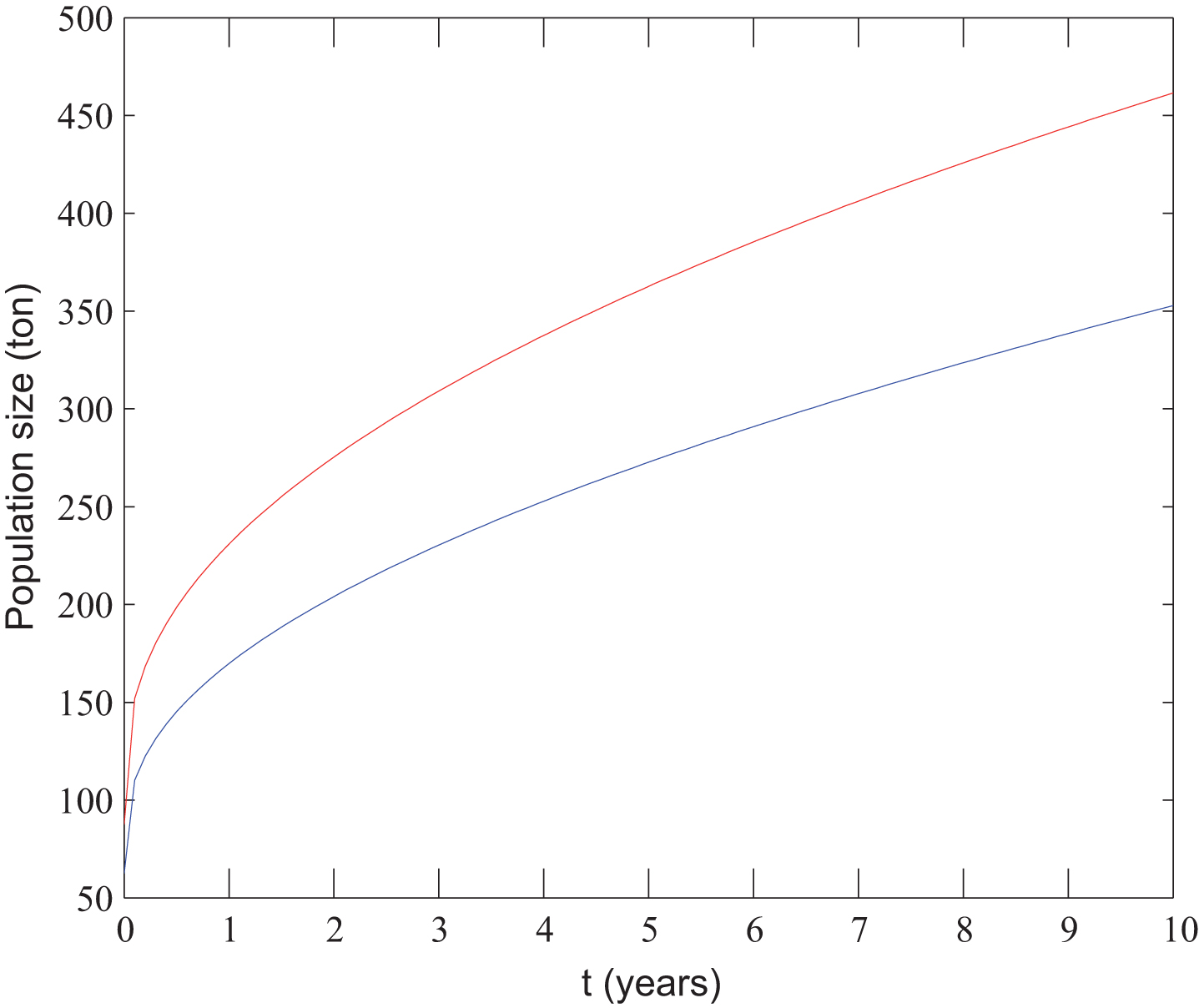In our numerical simulations we use the following parameters: β = 1, m = 0.01, r = 0.5, ω = 0.5 ∈ Ω = (0, 1) , α = 0.25, x₀ (ω) = (100ω, 150ω, 200ω) , and the overcrowding rate c = 0.0005 . The solution of (4.26-F) with the above hypothetical data is shown in Fig. 3.

Fig.1

The population size of fish (ton) without overcrowding of (4.26-F) with respect to time (years)

Fig.2

The population size of fish (ton) without harvesting of (4.26-F) with respect to time (years)

Fig.3

The population size of fish (ton) with overcrowding and harvesting of (4.26-F) with respect to time (years)

Example 4.6. From the crisp problem (4.26), in this example we choose a form for the corresponding random fuzzy fractional initial value problem as follows: $R L D_{0^{+}}^{α} x (t, ω) + c x^{2} (t, ω) + H \overset{[0, b], P .1}{=} (β - m) x (t, ω) ⊖ \frac{t^{- α}}{Γ (1 - α)} x (0, ω), x (0, ω) \overset{P .1}{=} x_{0} (ω),$ (4.28)

where (β - m) is to be assumed negative, H ∈ E is the harvest rate. In the sequel, we solve (4.26-F-2) in the case of x_1-α (t, ω) is d-decreasing for $ℙ -$ a.a. ω on [0, b]. If $(β - m) / c > \sqrt{4 \bar{H} (r) / c}$ and $λ_{i} \overset{ℙ . 1}{<} {\underline{x}}_{0} (ω, r) \overset{ℙ . 1}{\leq} {\bar{x}}_{0} (ω, r)$ (see λ_i above), then we obtain d-decreasing solution of (4.26-F-2), $[x_{FO} (t, ω)]^{r} = [\underline{x} (t, ω, r), \bar{x} (t, ω, r)],$ as follows: $\begin{matrix} \underline{x} (t, ω, r) & = \frac{({\underline{x}}_{0} (ω, r) - λ_{2}) λ_{1} exp (c Δ_{2} \frac{t^{α}}{Γ (α + 1)}) + λ_{2} (λ_{1} - {\underline{x}}_{0} (ω, r))}{({\underline{x}}_{0} (ω, r) - λ_{2}) exp (c Δ_{2} \frac{t^{α}}{Γ (α + 1)}) + (λ_{1} - {\underline{x}}_{0} (ω, r))}, \\ \bar{x} (t, ω, r) & = \frac{({\bar{x}}_{0} (ω, r) - λ_{4}) λ_{3} exp (c Δ_{1} \frac{t^{α}}{Γ (α + 1)}) + λ_{4} (λ_{3} - {\bar{x}}_{0} (ω, r))}{({\bar{x}}_{0} (ω, r) - λ_{4}) exp (c Δ_{1} \frac{t^{α}}{Γ (α + 1)}) + (λ_{3} - {\bar{x}}_{0} (ω, r))} . \end{matrix}$ In our numerical simulations we use the following parameters: β = 0.5, m = 1, r = 0.5, ω = 0.9 ∈ Ω = (0, 1) , α = 0.5, x₀ (ω) = (15ω, 30ω, 45ω) , and the overcrowding rate c = 0.1 . The solution of (4.26-F-2) with the above hypothetical data is shown in Fig. 4.

Fig.4

The population size of fish (ton) with overcrowding and harvesting of (4.26-F-2) with respect to time (years)

In the above examples we also consider the fuzzy fish population growth model by assuming that fish population size, the birth rate and the death rate are all fuzzy-valued. We can see the following examples.

Example 4.7. Let $k \in ℝ^{+}$ be the environmental carrying capacity of the resource population and let λ ∈ E be the growth rate of fish. We consider the random fuzzy fish proportional harvesting model given

${\begin{matrix} RL D_{0^{+}}^{α} x (t, ω) + \frac{λ}{k} x^{2} (t, ω) \\ + φ f (x (t, ω)) \overset{[0, b], ℙ . 1}{=} λ x (t, ω) ⊖ \frac{t^{- α}}{Γ (1 - α)} x (0, ω), \\ x (0, ω) \overset{ℙ . 1}{=} x_{0} (ω), \end{matrix}$ (4.29)

where $φ \in ℤ^{+}$ is the harvester of population size x and f (u) ∈ E is the harvesting rate for each person of u by individuals of φ. In this example we consider some proportion H ∈ E of u for the proportional harvesting model is harvested by each individual of φ, that is, we can take f (u) = Hu. In the sequel, we solve (4.29) under assuming that $[λ]^{r} = [\underline{λ} (r), \bar{λ} (r)]$ is positive i.e., $\underline{λ} (r), \bar{λ} (r) > 0$ , and in the case of x_1-α (t, ω) is d-increasing for $ℙ -$ a.a. ω on [0, b]. If $\underline{H} (r) < \underline{λ} (r) / φ$ and $\bar{H} (r) < \bar{λ} (r) / φ$ for r ∈ [0, 1], then we obtain d-increasing solution of (4.29), $[x_{FO} (t, ω)]^{r} = [\underline{x} (t, ω, r), \bar{x} (t, ω, r)],$ as follows: $\begin{matrix} \underline{x} (t, ω, r) = \frac{\underline{x} (0, ω, r) (1 - \frac{\underline{H} (r)}{\underline{λ} (r)} φ) k}{((1 - \frac{\underline{H} (r)}{\underline{λ} (r)} φ) k - \underline{x} (0, ω, r)) exp (- \underline{λ} (r) (1 - \frac{\underline{H} (r)}{\underline{λ} (r)} φ) \frac{t^{α}}{Γ (α + 1)}) + \underline{x} (0, ω, r)}, \\ \bar{x} (t, ω, r) = \frac{\bar{x} (0, ω, r) (1 - \frac{\bar{H} (r)}{\bar{λ} (r)} φ) k}{((1 - \frac{\bar{H} (r)}{\bar{λ} (r)} φ) k - \bar{x} (0, ω, r)) exp (- \bar{λ} (r) (1 - \frac{\bar{H} (r)}{\bar{λ} (r)} φ) \frac{t^{α}}{Γ (α + 1)}) + \bar{x} (0, ω, r)} . 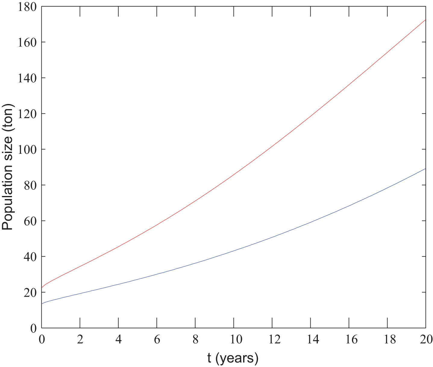\end{matrix}$ In our numerical simulations we use the following parameters: r = 0.5, ω = 0.9 ∈ Ω = (0, 1) , α = 0.75, φ = 10, k = 1000, x₀ (ω) = (10ω, 20ω, 30ω) , the growth rate in fuzzy environment λ = (0.3, 0.5, 0.8) and the harvesting rate H = (0.001, 0.003, 0.005). The d - increasing solution of (4.29) (or the population size of fish with respect to t) with the above hypothetical data is shown in Fig. 5.

Fig.5

The population size of fish (ton) of problem (4.29) with respect to time (years)

Example 4.8. Similarly, we also consider the fish proportional harvesting model in fuzzy environment given

${\begin{matrix} RL D_{0^{+}}^{α} x (t, ω) \overset{[0, b], ℙ . 1}{=} λ x (t, ω) ⊖ \frac{λ}{k} x^{2} (t, ω) \\ + (- 1) φ Hx (t, ω) + (- 1) \frac{t^{- α}}{Γ (1 - α)} x (0, ω), \\ x (0, ω) \overset{ℙ . 1}{=} x_{0} (ω), \end{matrix}$ (4.30) where $[λ]^{r} = [\underline{λ} (r), \bar{λ} (r)]$ is negative i.e., $\underline{λ} (r), \bar{λ} (r) < 0$ . In this example we solve (4.30) in the case of x_1-α (t, ω) is d-decreasing for $ℙ -$ a.a. ω on [0, b]. If $\underline{H} (r) < \bar{λ} (r) / φ$ and $\bar{H} (r) < \underline{λ} (r) / φ$ for r ∈ [0, 1], then we get d-decreasing solution of (4.30), $[x_{FO} (t, ω)]^{r} = [\underline{x} (t, ω, r), \bar{x} (t, ω, r)],$ asfollows: $\begin{matrix} \underline{x} (t, ω, r) = \frac{\underline{x} (0, ω, r) (1 - \frac{\underline{H} (r)}{\bar{λ} (r)} φ) k}{((1 - \frac{\underline{H} (r)}{\bar{λ} (r)} φ) k - \underline{x} (0, ω, r)) exp (- \bar{λ} (r) (1 - \frac{\underline{H} (r)}{\bar{λ} (r)} φ) \frac{t^{α}}{Γ (α + 1)}) + \underline{x} (0, ω, r)}, \\ \bar{x} (t, ω, r) = \frac{\bar{x} (0, ω, r) (1 - \frac{\bar{H} (r)}{\underline{λ} (r)} φ) k}{((1 - \frac{\bar{H} (r)}{\underline{λ} (r)} φ) k - \bar{x} (0, ω, r)) exp (- \underline{λ} (r) (1 - \frac{\bar{H} (r)}{\underline{λ} (r)} φ) \frac{t^{α}}{Γ (α + 1)}) + \bar{x} (0, ω, r)} . 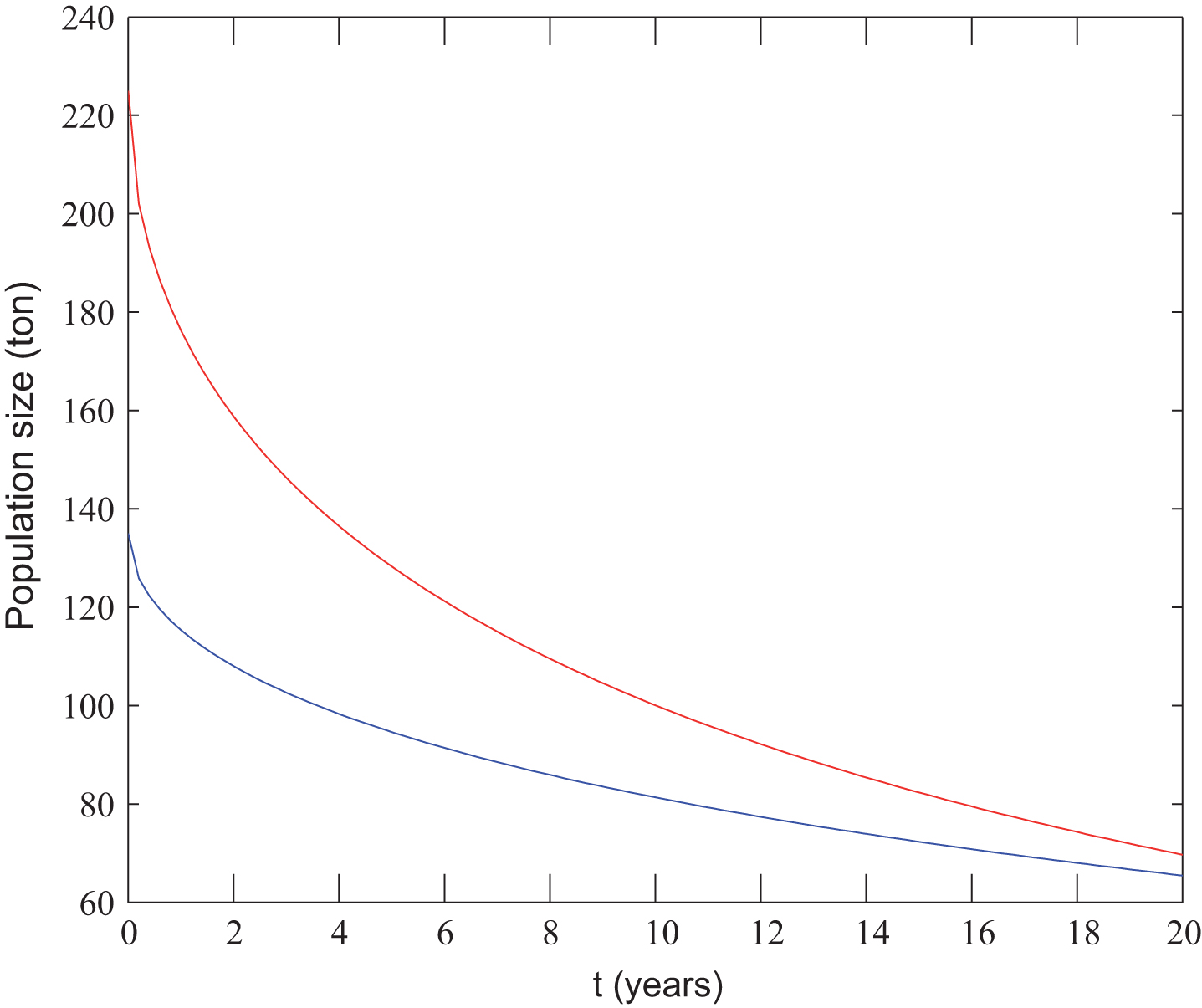\end{matrix}$ In our numerical simulations we use the following parameters: r = 0.5, ω = 0.9 ∈ Ω = (0, 1) , α = 0.5, φ = 2, k = 1000, x₀ (ω) = (100ω, 200ω, 300ω) , the growth rate in fuzzy environment λ = (-0.3, - 0.2, - 0.1) and the harvesting rate H = (0.002, 0.006, 0.010). The d - decreasing solution of (4.29) (or the population size of fish with respect to t) with the above hypothetical data is shown in Fig. 6.

Fig.6

The population size of fish (ton) of problem (4.30) with respect to time (years)

5 Conclusions

In this paper we investigate the existence and uniqueness results of solution of an initial value problems for random fuzzy differential equations with Riemann-Liouville fractional derivative. In addition, method to find solution of fractional fuzzy differential equations with Riemann-Liouville derivative and initial condition $x (a, ω) \overset{ℙ . 1}{=} x_{0} (ω)$ is proposed. The main usefulness of this method is being able to find the explicit solution of an initial value problem for random fuzzy differential equation with fractional order by using the solution of an integer-order fuzzy differential equation. We also use this method to find the exact solutions of the fish proportional harvesting model with two kinds of uncertainties: fuzziness and randomness. In recent years various advanced technique have been proposed to solve integer order fuzzy differential equations numerically, but for fractional fuzzy differential equations are not as strong as them. Therefore, by using the above approach we can establish the numerical methods for fuzzy fractional differential equations through the numerical methods for integer-order fuzzy differential equations. In future we plan to apply this approach to solve fuzzy fractional differential equations numerically.

Footnotes

Acknowledgments

The authors are very grateful to the referees for their valuable suggestions, which helped to improve the paper significantly. This research is funded by Vietnam National Foundation for Science and Technology Development (NAFOSTED) under grant number 101.02-2018.311.

References

Agarwal

R.P.

, Lakshmikantham

, Nieto

J.J.

, On the concept of solution for fractional differential equations with uncertainty, Nonlinear Analysis: (TMA) 72 (2010), 2859–2862.

Agarwal

R.P.

, Arshad

, ORegan

, Lupulescu

, Fuzzy fractional integral equations under compactness type condition,, Frac Cal and App Anal 15 (2012), 572–590.

Agraz

P.T.

, On Borel measurability and large deviations for fuzzy random variables,, Fuzzy Sets and Systems 157 (2006), 2558–2568.

Alikhani

, Bahrami

, Global solutions for nonlinear fuzzy fractional integral and integro differential equations, Commun Nonlinear Sci Numer Simulat 18 (2013), 2007–2017.

Allahviranloo

, Gouyandeh

, Armand

, Fuzzy fractional differential equations under generalized fuzzy Caputo derivative, Journal of Intelligent & Fuzzy Systems 26 (2014), 1481–1490.

Allahviranloo

, Salahshour

, Abbasbandy

, Explicit solutions of fractional differential equations with uncertainty, Soft Comput Fus Found Meth Appl 16 (2012), 297–302.

T.V.

, Vu

, Hoa

N.V.

, Applications of contractive-like mapping principles to interval-valued fractional integro-differential equations, Journal of Fixed Point Theory and Applications 19 (2017), 2577–2599.

A.T.V.

, Vu

, Hoa

N.V.

, A new technique to solve the initial value problems for fractional fuzzy delay differential equations, Advances in Difference Equations 2017 (2017), 181.

Arshad

, Lupulescu

, On the fractional differential equations with uncertainty, Nonlinear Analysis: (TMA) 74 (2011), 85–93.

10.

Bede

, Stefanini

, Generalized differentiability of fuzzy-valued functions, Fuzzy Sets and Systems 230 (2013), 119–141.

11.

Bhaskar

T.G.

, Lakshmikantham

, Leela

, Fractional differential equations with a Krasnoselskii– Krein type condition, Nonlinear Analysis: Hybrid Systems 3 (2009), 734–737.

12.

Colubi

, Domínguez-Menchero

J.S.

, López-Díaz

, Ralescu

D.A.

, A D_E[0, 1] representation of random upper semicontinuous functions, Proc Amer Math Soc 130 (2002), 3237–3242.

13.

Hoa

N.V.

, Fuzzy fractional functional differential equations under Caputo gH differentiability, Commun Nonlinear Sci Numer Simulat 22 (2015), 1134–1157.

14.

Hoa

N.V.

, Vu

, Duc

T.M.

, Fuzzy fractional differential equations under Caputo- Katugampola fractional derivative approach, Fuzzy Sets and Systems (2018).

15.

Hoa

N.V.

, Fuzzy fractional functional integral and differential equations, Fuzzy Sets and Systems 280 (2015), 58–90.

16.

Hoa

N.V.

, Lupulescu

, O’Regan

, Solving interval-valued fractional initial value problems under Caputo gH-fractional differentiability, Fuzzy Sets and Systems 309 (2017), 1–34.

17.

Hoa

N.V.

, Lupulescu

, O’Regan

, A note on initial value problems for fractional fuzzy differential equations, Fuzzy Sets and Systems 347 (2018), 54–69.

18.

Hoa

N.V.

, Existence results for extremal solutions of interval fractional functional integro-differential equations, Fuzzy Sets and Systems 347 (2018), 29–53.

19.

Kaleva

, A note on fuzzy differential equations, Nonlinear Anal 64 (2006), 895–900.

20.

Kilbas

A.A.

, Srivastava

H.M.

, Trujillo

J.J.

, Theory and applications of fractional differential equations, Amesterdam: Elsevier Science B.V, 2006.

21.

Klement

E.P.

, Puri

M.L.

, Ralescu

D.A.

, Limit theorems for fuzzy random variables, Proc Roy Soc Lond A 407 (1986), 171–182.

22.

Kruse

, Meyer

K.D.

, Statistics with Vague Data, Kluwer, Dordrecht, 1987.

23.

Kwakernaak

, Fuzzy random variables. Part I: Definitions and theorems, Inform Sci 15 (1978), 1–29.

24.

Lakshmikantham

, Theory of fractional functional differential equations, Nonlinear Analysis: Theory, Methods & Applications 69 (2008), 3337–3343.

25.

Lakshmikantham

, Leela

, A Krasnoselskii-Krein-type uniqueness result for fractional differential equations, Nonlinear Analysis: TMA 71 (2009), 3421–3424.

26.

Lakshmikantham

, Mohapatra

R.N.

, Theory of fuzzy differential equations and applications, Taylor & Francis, London, 2003.

27.

Lakshmikantham

, Vatsala

A.S.

, Theory of fractional differential inequalities and applications, Communications in Applied Analysis 11 (2007), 395–402.

28.

Long

H.V.

, Son

N.T.K.

, Hoa

N.V.

, Fuzzy fractional partial differential equations in partially ordered metric spaces, Iranian Journal of Fuzzy Systems 14 (2017), 107–126.

29.

Long

H.V.

, Son

N.K.

, Tam

H.T.

, Yao

J.C.

, Ulam Stability for fractional partial integrodifferential equation with uncertainty, Acta Math Vietnam 42 (2017), 675–700.

30.

Long

H.V.

, Son

N.K.

, Tam

H.T.

, The solvability of fuzzy fractional partial differential equations under Caputo gH-differentiability, Fuzzy Sets Systems 309 (2017), 35–63.

31.

Long

H.V.

, On random fuzzy fractional partial integro-differential equations under Caputo generalized Hukuhara differentiability, Computational and Applied Mathematics 37 (2018), 2738–2765.

32.

Long

H.V.

, Dong

N.P.

, An extension of Krasnoselskiis fixed point theorem and its application to nonlocal problems for implicit fractional differential systems with uncertainty, Journal of Fixed Point Theory and Applications 20 (2018), 37.

33.

Lupulescu

, Hoa

N.V.

, Existence and uniqueness of solutions for random fuzzy fractional integral and differential equations, Journal of Intelligent & Fuzzy Systems 29 (2015), 27–42.

34.

Lupulescu

, Fractional calculus for interval-valued functions, Fuzzy Set and Systems 265 (2015), 63–85.

35.

Mazandarani

, Kamyad

A.V.

, Modied fractional Euler method for solving fuzzy fractional initial value problem, Communications in Nonlinear Science and Numerical Simulation 18 (2013), 12–21.

36.

Mazandarani

, Najariyan

, Type-2 fuzzy fractional derivatives, Communications in Nonlinear Science and Numerical Simulation 19 (2014), 2354–2372.

37.

Malinowski

M.T.

, On random fuzzy differential equations, Fuzzy Sets and Systems 160 (2009), 3152–3165.

38.

Malinowski

M.T.

, Random fuzzy differential equations under generalized Lipschitz condition, Nonlinear Analysis: RealWorld Applications 13 (2012), 860–881.

39.

Malinowski

M.T.

, Existence theorems for solutions to random fuzzy differential equations, Nonlinear Analysis: TMA 73 (2010), 1515–1532.

40.

Malinowski

M.T.

, Random fuzzy fractional integral equations - theoretical foundations, Fuzzy sets and Systems 265 (2015), 39–62.

41.

Malinowski

M.T.

, Fuzzy and set-valued stochastic differential equations with local Lipschitz condition, IEEE Transactions on Fuzzy Systems 23 (2015), 1891–1898.

42.

Malinowski

M.T.

, Agarwal

R.P.

, On solutions to set-valued and fuzzy stochastic differential equations, Journal of the Franklin Institute 352 (2015), 3014–3043.

43.

Malinowski

M.T.

, Some properties of strong solutions to stochastic fuzzy differential equations, Information Sciences 252 (2013), 62–80.

44.

Malinowski

M.T.

, Itô type stochastic fuzzy differential equations with delay, Systems & Control Letters 61 (2012), 692–701.

45.

Malinowski

M.T.

, Strong solutions to stochastic fuzzy differential equations of Itô type, Mathematical and Computer Modelling 55 (2012), 918–928.

46.

Malinowski

M.T.

, Random fuzzy fractional integral equations-theoretical foundations, Fuzzy Sets and Systems 265 (2015), 39–62.

47.

Nguyen

H.T.

, A note on the extension principle for fuzzy sets, J Math Anal Appl 64 (1978), 369–380.

48.

Park

J.Y.

, Jeong

J.U.

, On random fuzzy functional differential equations, Fuzzy Sets and Systems 223 (2013), 89–99.

49.

Podlubny

, Fractional differential equation, San Diego:Academic Press, 1999.

50.

Puri

M.L.

, Ralescu

, Differential for fuzzy function, Journal of Mathematical Analysis and Applications 91 (1983), 552–558.

51.

Puri

M.L.

, Ralescu

D.A.

, The concept of normality for fuzzy random variables, Ann Probab 13 (1985), 1373–1379.

52.

Puri

M.L.

, Ralescu

D.A.

, Fuzzy random variables, J Math Anal Appl 114 (1986), 409–422.

53.

Salahshour

, Allahviranloo

, Abbasbandy

, Baleanu

, Existence and uniqueness results for fractional differential equations with uncertainty, Advances in Difference Equations 2012 (2012), 112.

54.

Salahshour

, Allahviranloo

, Abbasbandy

, Solving fuzzy fractional differential equations by fuzzy Laplace transforms, Communications in Nonlinear Science and Numerical Simulation 17 (2012), 1372–1381.

55.

Song

, Wu

, Existence and uniqueness of solutions to Cauchy problem of fuzzy differential equations, Fuzzy Sets and Systems 110 (2000), 55–67.

56.

, Dong

L.S.

and Hoa

N.V.

, Random fuzzy functional integro-differential equations under generalized Hukuhara differentiability, Journal of Intelligent & Fuzzy Systems 27 (2014), 1491–1506.

57.

, Ho , Lupulescu

and Hoa

N.V.

, Existence of extremal solutions to interval-valued delay fractional differential equations via monotone iterative technique, Journal of Intelligent & Fuzzy Systems 34 (2018), 2177–2195.

58.

, Hoa

N.V.

, Son

N.T.K.

, O’Regane

, Results on initial value problems for random fuzzy fractional functional differential equations, Filomat 32 (2018), 2601–2624.