An improved fuzzy time series forecasting model using the differential evolution algorithm

Abstract

Fuzzy time series modeling has recently become an interesting topic to study. Among fuzzy time series models, the Abbasov-Mamedova (AM) model has advantages over the others because it can forecast the value that is outside the min-max range of the original data. However, the performance of the AM model strongly depends on three parameters that are user-defined. In previous studies, the optimal parameters of the fuzzy time series models have been identified with a global optimization method. Surprisingly, optimizing the parameters of the Abbasov and Mamedova model has not been solved in spite of its advantages over the others. This paper presents a new approach to improve the performance of AM model based on the evolutionary algorithm. Particularly, the objective function is calculated as the Mean absolute percentage error which will be minimized using the differential evolution (DE) algorithm. The experiments on Azerbaijan’s population, Vietnam’s GDP and rice production demonstrate the feasibility and applicability of the proposed methods.

Keywords

fuzzy time series differential evolution optimization forecast MAPE

1 Introduction

Forecasting is a science of predicting the future by scientific analyzing the collected data. Due to the remarkable development of science, numerous forecasting models have been proposed and demonstrated their suitability and effectiveness, so far. Although these models have contributed significantly to the forecasting theory, they still have limitations in practical application. For instance, regression models (e.g. linear regression [18, 43]) require a number of assumptions that are not always valid, whereas the time series models (e.g. ARIMA [7]) perform poorly when there are abnormal changes or the time series is nonstationary. Similarly, various models [11 , 64] provided good results in considered data sets;.owever, we could not obtain the optimum solution for all cases, and most of them still have many disadvantages in real forecasting applications.

Based on the fuzzy theory of Zadeh [60], the fuzzy time series (FTS) introduced by Song and Chissom [51] is able to forecast without requiring any assumptions like regression and ARIMA. Recently, FTS has been an interesting topic and shown to be more efficient than any classical forecasting model. Using the fuzzy logical relationship table Chen [8] proposed a conventional fuzzy time series model, which is computationally easier than the method of Song and Chissom. Next, Chen [9] adapted the method in [8] for high-order fuzzy time series. Huarng and Yu [33] advanced a type 2 FTS model from the type 2 fuzzy set. Furthermore, Yu [59] proposed a weighted FTS model to resolve recurrent fuzzy relationships and assign appropriate weights to several fuzzy relationships, correctly reflecting their respective import. Abbasov and Mamedova [1] proposed the fuzzy time series model to forecast the population of Azerbaijan, where the first order difference of data is utilized. A list of researches which proposed fuzzy time series techniques to address the problem of forecasting can be found in [4 , 54]. Most of the above models define the universe of discourse based on the min and max values of the original data, then fuzzify the time series and select the defuzzified value of fuzzified prediction variables;.herefore, the forecasting values always fall into the limited domain of original data, that is, they are unsuitable when dealing with the nonstationary data. For example, after establishing fuzzy logical relationship groups, the Chen model [8] uses the following rule for forecasting the output y (t + 1) at the time point t + 1: $y (t + 1) {\begin{matrix} = \sum_{i}^{p} μ_{i} m_{i} & if \exists i : A_{j} \to A_{i} \\ = m_{j} & otherwise \end{matrix}$ (1) where p is the number of fuzzy sets or divided intervals, A_j is the record of year t in terms of a fuzzy set, m_i is the middle point of the interval i, μ_i = 1 if we have A_j →.A_i, otherwise μ_i = 0. It is obvious that the possible minimum and maximum outputs of y (t + 1) are m₁ and m_p, respectively, that is, the forecasting values always fall into this limited domain. On the other hand, instead of working with the original data, the Abbasov-Mamedova model (AM) performs the forecasting process on the first order difference V (t) and predicts Y (t + 1) by adding Y (t) with the forecast of V (t);.ence, it can handle a number of nonstationary time series data sets with high-quality forecasting results. Recently studies which have successfully applied the AM model to many practical applications are [1 , 48]. However, all of the above models including the AM model require a number of parameters to be provided by the user. This makes them suitable only for the cases that were studied and lose generality. To overcome this problem, a new researched direction combining fuzzy time series model and optimization algorithm has been developed.

Optimization algorithms can be decomposed into two major techniques: population-based algorithms and gradient-based searching algorithms. Recently, although there have been various population-based algorithms proposed in literature, it can be noted that the Genetic Algorithm (GA), the Particles Swarm Optimization (PSO) and the Differential Evolution (DE) are the three most popular ones. The GA [31] inspired by the natural choice and the survival of chromosomes which represent the solutions. To create new solutions, the GA utilizes some genetic operators termed as selection, crossover, and mutation. The objective is to find the best chromosome or solution after some termination conditions. The GA was performed well in many practical problems including computer vision [12], clustering [2, 55] and structural engineering problems [21, 23], etc. The PSO [35] focuses on the social behaviors of birds to solve the optimization problem. In the PSO, each solution is represented by a particle which has two main properties: the position and the velocity. The algorithm works to create new solutions through the movement of particles based on the velocity. The applications of PSO in various fields can be listed in [19 , 42]. The DE [52] also uses the chromosomes to represent the solutions and generates the new ones using genetic operators like the GA but the operators are not all exactly the same as those with the same names in the GA. In the DE, the mutation operator which combines three randomly selected vectors from the population to form mutation vector plays a key role in finding the global optimum and is very different with the same operator in the GA. The DE and its variations were successfully applied to many fields, such as civil engineering, pattern recognition, etc. [13 , 45]. In addition to the three above algorithms and their relevance, a large number of studies were proposed in various aspects including methodology and application [20 , 46]. The comparisons of the GA, the PSO, and the DE were presented in [34, 58] in which all authors concluded that the DE has the best global search ability. Based on the best of our knowledge as well as many empirical experiments, we also identify that the GA has good ability to find the global optimum but has a slow convergence speed;.he PSO has a fast convergence speed but is easily trapped into a local optimum;.he DE is the best one when it balances both searching global optimum and saving the computational cost.

Based on the optimization algorithms, many approaches were proposed to perform fuzzy time series. Aladag et al. [3] introduced an invariant fuzzy time series model in which the membership values in the fuzzy relationship matrix are computed using particle swarm optimization technique (optimize the determination phase). However, in this research, each particle represents a fuzzy relation matrix whose number of elements is equal to the square of the number of fuzzy sets;.ence, the optimal model is obtained at a cost of increased computational complexity. Another limitation of this research is that the PSO may easily get trapped in a local optimum, according to [63]. Bas et al. [6] proposed a modified genetic algorithm to find optimal interval lengths or fuzzy sets (optimize the fuzzification phase). It is well-known that the Genetic algorithm has a slow convergence speed;.s a result, this research either takes a high computational cost or cannot reach the global optimum if a specific number of iterations is used as the stopping condition. Other methods integrating the optimization algorithm to the fuzzy time series model [36, 49] had the same drawbacks, such as taking high complexity or being trapped to local optimum. Furthermore, it can be noted that most of the above methods were formed by derivation from the Chen model, the Yu model or other models solving the problem in the original data. None of them proposed a method for optimizing the Abbasov and Mamedova model (AM) in spite of its advantages as mentioned earlier. Because the Abbasov and Mamedova model can handle the data that tend to whether increase or decrease, continuously, using the first order difference of time series, optimizing its parameters is important to provide a more accurate model for prediction.

The AM model requires three parameters consisting of the number of equal-length intervals n, the positive integer w and the constant C to be carefully selected for different data sets. However, in the studies of [1 , 48], these parameters were chosen according to the author’s own experience. Hence, the built models can be unsuitable when dealing with various types of time series. For w, Song and Chissom [51] conducted a survey on the enrollment data and pointed out that the forecasting result will be better if we perform a less complex model, with a w value of two being optimal. However, this conclusion was only drawn from a small number of surveys and might lose generality. In addition, Ha et al. [28] proposed a two-stage algorithm for the AM model where the first stage identifies n, w and C before passing them to the AM model in the second stage. The major deficiency of this research is that the parameters n, w and C were separately examined and their interactions were not investigated. Therefore, a method that can evaluate the quality of the model when simultaneously changing the three parameters is highly desirable. Based on the above idea, this paper proposes a method for optimizing the quality of the AM model using the DE algorithm. We term the new model simply as the DEABB model in which the parameters n, w and C are selected so that the mean absolute percentage error, MAPE, is minimized. The contributions of this research are listed as follows:

In the DEABB, the optimization algorithm is applied to the AM model rather than the others;.herefore, the proposed method can forecast the values that fall outside the min-max range of the original data, whereas most of the previous models are not able to forecast those kinds of values.

In the DEABB, three parameters including n, w and C are optimized, where n denotes the number of intervals used in fuzzification phase;.C has effects on the value of membership function;.nd w represents the number of years used to establish the fuzzy relationship in determination phase. Therefore, the proposed method can optimize the model in both fuzzification and determination phases when the previous methods often optimize one of them.

The DE has a better convergence behavior in comparison with the GA and the PSO;.s a result, it can be expected that the proposed algorithm, DEABB, ensures both finding the global optimum and saving the computational cost thereby overcoming the drawbacks of existing methods.

In addition to academic contributions, the DEABB can yield good forecasting results when dealing with the real-world data, such as Vietnam’s GDP and rice production, etc. The gross domestic product (GDP) is one of the major measures of nation’s economic health, whereas the rice production forecasting is one of the most necessities for a successful agricultural economics. Therefore, providing a more accurate forecasting has a significant meaning for the government.

The proposed model is programmed in R, an open-source or free license that is easy for the user to refer, apply and modify.

Table 1 briefly summarizes some properties of the DEABB and previous methods to clarify the proposed method’s contributions. The remainder of this article is organized as follows. In Section 2, the preliminary issues of the fuzzy time series and the AM model are reviewed. The DE algorithm as well as the proposed method is introduced in Section 3, illustrated and applied in Section 4. Section 5 is the conclusion.

Table 1

The comparison of the DEABB and the existing algorithm properties

Method	Forecast outside the original data	Phase of optimization	Reach global optimum	Computational cost
The AM model	Yes	No	-	Low
The model in [8]	No	No	-	Low
The model in [32]	No	No	-	Low
The model in [3]	Yes	Determination	Not good	High
The model in [6]	No	Fuzzification	Good	High
The model in [10]	No	Fuzzification	Good	High
The model in [36]	No	Fuzzification	Not good	Low
The DEABB	Yes	Both two phases	Good	Low

2 The Abbasov-Mamedova Model

2.1 The fuzzy time series

Let Y (t) ∈.R, t = 0, 1, 2, ….e a time series, with a generic element, y_t. If μ_A (y_t) is the membership function which is a mapping from the universe containing Y (t) into [0, 1] and F (t) = {μ_A (y₀), μ_A (y₁), μ_A (y₂), …} is a collection of μ_A (y_t) then F (t) is called a fuzzy time series.

2.2 The Abbasov-Mamedova model

Given the historical data X_t which have m number of records, t = 1, 2, …, m, the AM model suggested by Abbasov and Mamedova [1] is formally presented by the following process.

Step 1: Compute the variation V_t between two continuous historical data;.hen define the universal set U. This can be formulated mathematically as: $V_{t} = X_{t} - X_{t - 1}$ (2) $U = [V_{min} - D_{1}, V_{max} + D_{2}]$ (3) where V_min is the smallest variation, V_max is the greatest variation, D₁ and D₂ are positive numbers.

Step 2: Partition the universe of discourse U into n equal length intervals u_i, i = 1, 2, …, n, such that each interval u_i contains at least one point from V_t. Then find the middle point $u_{m}^{i}$ of interval u_i, i = 1, 2, …, n.

Step 3: Define the fuzzy set A_i, i = 1, 2, …, n, on the universe of discourse U by the following formula: $μ_{A_{i}} (u) = \frac{1}{1 + {[C \times (u - u_{m}^{i})]}^{2}},$ (4) where u is a generic element of universal set U, $u_{m}^{i}$ is the middle point of the corresponding interval u_i, (i = 1, 2, …, n) and C is a constant.

Step 4: Find out the degree to which the variation V_t belongs the fuzzy set A_i or map the first order differences into fuzzy values by Formula 4.

Step 5: Select an integer w, 1 <.w <.l, where l is the number of years, prior to the current year included in experimental evaluation. Based on the chosen w and Mamdani fuzzy inference system, we then establish an operation matrix O^w (t) of size i ×.j (here i, which is the number of rows, conforms to the sequence of years t - 2, t - 3, …, t - w;.j, which is the number of columns, conforms to the number of fuzzy sets) and a criteria matrix K (t) of size 1 ×.j, which corresponds to the fuzzy value at the time point t - 1. After that, the relationship matrix R (t) is given as: $R (t) [i, j] = O^{w} [i, j] \cap K (t) [j],$ (5) or $R (t) = O^{w} (t) \otimes K (t) = [\begin{matrix} R_{11} & R_{12} & . . . & R_{1 j} \\ R_{21} & R_{22} & . . . & R_{2 j} \\ . . . & . . . & . . . & . . . \\ R_{i 1} & R_{i 2} & . . . & R_{ij} \end{matrix}],$ (6) where O^w (t) is the operation matrix, K (t) is the criteria matrix, ⊗.s the min operator (∩). Once the relationship matrix R (t) is ready calculated, we define F (t) which is the fuzzy forecasting of variations for the year t and is formulated as follows. $\begin{matrix} F (t) & = & [max (R_{11}, \dots, R_{i 1}), \dots, max (R_{1 j}, \dots, R_{ij})] \\ = & [μ_{A_{1}} (V_{t}), μ_{A_{2}} (V_{t}), \dots, μ_{A_{m}} (V_{t})] . \end{matrix}$ (7)

Step 6: Defuzzify F (t) according to the following formula. $V (t) = \frac{\sum_{i = 1}^{m} μ_{A_{i}} (V_{t}) \times u_{m}^{i}}{\sum_{i = 1}^{m} μ_{A_{i}} (V_{t})},$ (8) where μ_{A
_i} (V_t) is the value of membership function of the forecast variation in interval i, V (t) is the defuzzified forecast variation.

Based on the defuzzified forecast variation V (t) and the previous value X (t - 1), the forecasted output X (t) is obtained using the formula: $X (t) = X (t - 1) + V (t) .$ (9)

2.3 Evaluating a fuzzy time series model

Let X and $\hat{X}$ , the row vectors of dimension m, be the actual data and the predicted data, respectively. We formalize the criteria for evaluating a fuzzy time series model as follows. Mean absolute error: $MAE = \frac{1}{m} \sum_{i = 1}^{m} | {\hat{X}}_{i} - X_{i} | .$ (10) Mean squared error: $MSE = \frac{1}{m} \sum_{i = 1}^{m} {({\hat{X}}_{i} - X_{i})}^{2} .$ (11) Mean absolute percentage error: $MAPE = \frac{1}{m} \sum_{i = 1}^{m} (\frac{| {\hat{X}}_{i} - X_{i} |}{X_{i}} . 100) .$ (12)

By applying the above criteria, the forecasted result of a model can be evaluated. The model with the lowest MAE, MSE, MAPE should be used for forecasting.

3 The differential evolution algorithm and proposed method

3.1 The differential evolution algorithm

The differential evolution algorithm, DE, is a well-known global search method based on population, designed to deal with the problems which can be continuous and discrete [52]. The DE dominance is proved through the effective and robust performance both in benchmark and real-world problems. There are four major phases in the procedure of DE including initialization, mutation, crossover and selection.Initialization In the initialization phase of the DE, NP individuals are generated through a random sampling technique which can be formulated mathematically as: $x_{i, j} = x_{j}^{l} + rand [0, 1] \times (x_{j}^{u} - x_{j}^{l}) .$ (13) where i = 1, 2, …, NP ;.j = 1, 2, …, N, $x_{j}^{l}$ and $x_{j}^{u}$ are respectively the lower and upper bounds of x_j;.and [0, 1] is the real number having the uniform distribution within [0, 1];.NP is the population size.Mutation For every individual x_i, we generate a mutant vector v_i using the mutation operation. Some mutation operations regularly used in the DE are shown as follows.

rand/1: $v_{i} = x_{r_{1}} + F \times (x_{r_{2}} - x_{r_{3}})$ (14)

rand/2: $v_{i} = x_{r_{1}} + F \times (x_{r_{2}} - x_{r_{3}}) + F \times (x_{r_{4}} - x_{r_{5}})$ (15)

best/1: $v_{i} = x_{best} + F \times (x_{r_{1}} - x_{r_{2}})$ (16)

where integers r₁, r₂, r₃, r₄, r₅ are randomly selected from {1, 2, …, NP }.nd must satisfy r₁ ≠.r₂ ≠.r₃ ≠.r₄ ≠.r₅ ≠.i;.F is the scale factor and randomly chosen within [0, 2];.x_best is the best individual in the current population.

Crossover

After completing mutation, we calculate a trial vector u_i for every target vector x_i by substituting some components of the vector x_i by some components of the mutant vector v_i. The calculation can be carried out by the binomial crossover operation which can be formulated mathematically as: $u_{ij} = {\begin{matrix} v_{ij} if rank [0, 1] \leq CR \\ x_{ij} otherwise \end{matrix}$ (17) where i∈.#x007B;., 2, …, NP };.j∈.#x007B;., 2, …, N }.nd CR is the crossover control parameter chosen within [0, 1].

Selection

Finally, each trial vector u_i is compared to its target vector x_i. The vector providing better objective function value is reserved for the next generation. The search will be executed as long as g <.maxiter, where g is the current iteration and maxiter is the maximum number of iterations.

3.2 The proposed algorithm

As mentioned earlier, the AM model performance relies on the choice of parameters n, w, and C. The proposed method uses the concept of the optimization problem for the fuzzy time series problem. In particular, we propose a method to minimize the mean absolute percentage error for the AM model using the DE algorithm. Initially, because the DE defines a solution as a chromosome, it requires the solutions of n, w, and C to be encoded. The encoding phase is summarized in Fig. 1. It can be clearly seen from Fig. 1 that a possible solution is defined as a chromosome containing three genes which represent the values of n, w and C, i.e. the size of the chromosome will be the same as the number of variables. The MAPE can be viewed as the implicit objective function of n, w, and C, i.e., the values of MAPE can be different with different chromosomes.

Fig.1

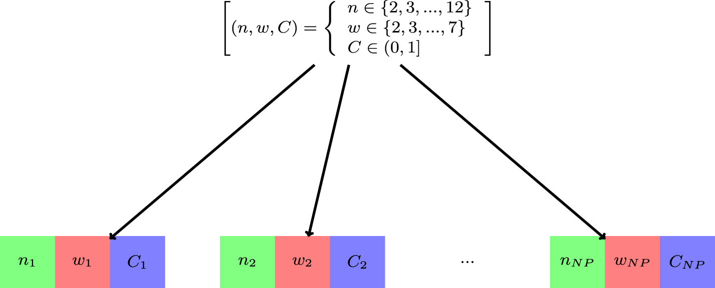
The illustration for the encoding.

After completion of encoding phase, the chromosomes or feasible solutions can be processed by the mutation, crossover and selection operators. Through any iteration i, only a fixed number of solutions n, w, and C can be selected for the next iteration. After maxiter iterations, a chromosome which provides the smallest MAPE will be considered as the best solution and then the optimal n, w, and C are given as input into the main phase of AM model. The overall process of the proposed algorithm, DEABB, is outlined by the Algorithm 1.

Algorithm 1:

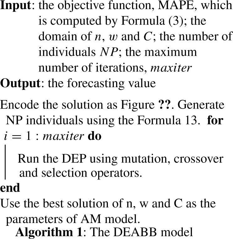
The DEABB model

4 Numerical examples

In this section, the DEABB model is employed to solve forecasting problems. The outline of this section is briefly presented as follows. Firstly, the detail of each data set will be presented. Secondly, we present the investigation of the effects of the mutant factor F, crossover control parameter CR, and the maximum number of iterations maxiter on the optimal solution. Thirdly, the comparison between the DEABB and the others including the models in [1 , 32], the GAABB model and the PSOABB model is designed to measure the effectiveness of the proposed method. Further, the paired samples t-test is performed to validate whether the difference is significant or not. Finally, the proposed model is applied to out-of-sample forecasting.

4.1 The data sets

To evaluate the performance of the proposed method, three experiments are presented. In Experiment 1, we adopted the well-known data of the historical population of Azerbaijan [1] to illustrate the proposed method and test its performance. The Experiment 2 and the Experiment 3 are used to test the robustness of the DEABB model when dealing with the real-world data, Vietnam’s GDP and rice production. For this purpose, Vietnam’s GDP per capita (USD) from 1990 to 2015 and rice production (thousand tons) from 1990 to 2014, are adopted. The original data of all experiments can be found in [1] and http://data.worldbank.org).

4.2 The effects of the parameters F, CR, and maxiter on the optimal solution

Before the DE algorithm can perform well, a set of parameters including the number of individuals NP, the scale factor F, the crossover control parameter CR, the maximum number of iterations maxiter, require to be provided by the user. To obtain satisfactory parameters of F, CR, and maxiter for all experiments, a survey of the effects of parameters on the optimal solutions is presented in this subsection. Based on the obtained results, a suitable set of parameters can be indicated. According to [5, 44], the number of chromosomes or the cardinality of the individual set in each iteration should be set as 10*d where d is the problem dimensions, i.e. NP=30 in this paper. With NP = 30 and a specific number of iterations, the effect of the mutation operator is described in Fig. 2. The data of Azerbaijan population in Experiment 1 have a simple linear trend;.ence, it can be clearly seen from Fig. 2a that the DE can find the solution that has the minimum MAPE in almost all cases of F. In case of more complex data, such as the Experiment 2 and the Experiment 3, the effect of F on the optimum solution is clarified. Using a small value of F, the DE cannot explore the search space effectively, as a result, cannot reach the optimal solution on the completion of the algorithm. In contrast, using a high value of F results in the occasional movement;.ence, the DE has a weak exploitation behavior for reaching the global optimum in the later steps. As evidenced by Fig. 2b and Fig. 2c, the solutions of the DE are not good when F >..7 and F >. in Experiment 2 and Experiment 3, respectively. In this case, F = 1 would be a stable choice, suitable for the data sets in this work.

Fig.2

The effects of F.

For the crossover control parameter CR, the trial vector tends to be the same with the mutant vector when CR →. and the same with the target vector when CR →.. Figure 3 shows how the MAPE changes when increasing CR value. According to Fig. 3, the same trends are obtained for Experiment 1 and Experiment 2 when the global optimal values can be reached in almost all cases. The best CR in Experiment 3 falls in the interval [0.3, 0.7]. According to the obtained results, a CR value which falls within the range [0.3, 0.7] would give the optimal MAPE. In this case, CR = 0.5 is used in this paper to balance the properties of the target and the mutant vectors.

Fig.3

The effects of CR.

Using the found F and CR, we continue to survey the effect of the maximum number of iterations maxiter. Figure 4 shows the MAPE of different maxiter values for the data sets used in the three experiments. It can be seen from Fig. 4 that with the maxiter ≥.0, the global optimum can be reached in all experiments. Based on the obtained results, we choose maxiter = 60 to reduce the computational cost as much as possible. For other applications, users can choose a larger maxiter to ensure convergence to the global minimum.

Fig.4

The effects of maxiter.

4.3 The comparison of the DEABB and other methods

This subsection shows the comparison for the DEABB with other well-known fuzzy time series models for the three data sets. In particular, the performance of the proposed method is compared with those of the AM model [1], the Chen’s model [8], the Huarng’s model [32]. Also, we provide the extensive evaluations and comparisons with other well-known optimization methods such as the GA and the PSO, that is, we compare the performance of the DEABB model with those of the ones termed GAABB model and PSOABB model. To ensure the fairness, in our experiments for DEABB, GAABB and PSOABB, we consider the same stopping criterion, maxiter = 60. The validation is performed using the MAPE, MAE, MSE criteria as well as the paired Student’s t-test. Figure 5 shows the forecasting results of the DEABB and comparative models for the three data sets. Table 2 shows the comparison of some forecasting performance measures for the DEABB with other models. According to the forecasting results, we can group the models into two groups: Group 1 includes the models of Chen and Huarng;.roup 2 includes the AM-based models. The Chen model calculates the output using the simple average of the middle points;.ence, it results in a rough forecast and degrades the forecasting quality. The same deficiency is also found in the Huarng’s model. The AM-based models including the original AM, the GABBB, the PSOABB and the DEABB models utilize the sum of the original data and the first difference forecast as the output and it is because of this that the forecasting results are smooth and can adapt to the original data. Consequently, their performance are better than those of the Chen and the Huarng models. The DEABB model is more efficient than the AM model when it provides the lower MAE, MSE, and MAPE as shown in Table 2. This is due to the fact that the DEABB model not only can adapt to the original data as the AM model but also can optimize the AM model parameters.

Fig.5

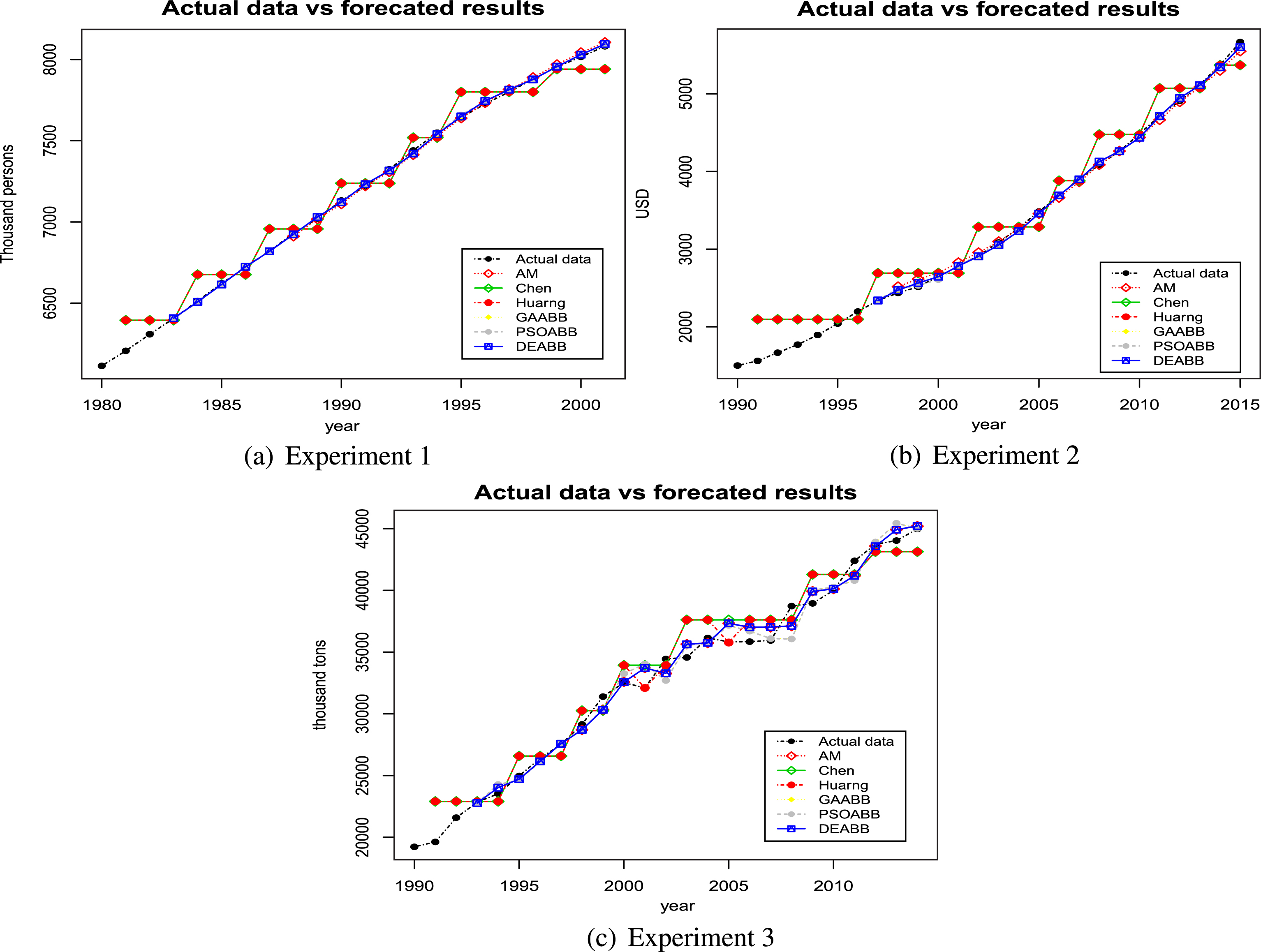
The actual data and forecasted results for all experiments.

Table 2

Forecasting results of comparative models

	Experiment 1			Experiment 2			Experiment 3
MAE	MAPE	MSE	MAE	MAPE	MSE	MAE	MAPE	MSE
AM	15.007	0.197	290.459	42.942	1.224	2834.763	867.224	2.401	1016128.000
Chen	77.756	1.099	8835.054	201.552	7.860	62332.370	1373.772	4.375	2471075.000
Huarng	77.756	1.099	8835.054	201.552	7.860	62332.370	1225.760	3.937	2198843.000
GAABB	8.959	0.120	107.705	25.033	0.693	1023.306	831.390	2.380	1168167.000
PSOABB	9.576	0.130	122.381	25.147	0.697	991.016	831.524	2.381	1169138.000
DEABB	8.953	0.120	107.650	24.320	0.665	992.140	719.418	2.056	797072.100

To perform the comparisons with the GAABB and PSOABB models, we first run the three algorithms with 200 iterations. This would be very useful to obtain an overview of the convergence behavior as shown in Fig. 6. Figure 6 gives us some useful and intuitive views and we can draw some remarkable insights: (i) In the first two experiments, it can be seen that both the GA and the DE can reach the global optimum but the DE has the faster convergence speed. To reach the global optimum, it takes the DE about 5 iterations for Experiment 1 and 20 iterations for Experiment 2;.he corresponding number of iterations for the GA are about 50 and 70. Clearly, taking high computational cost is the major deficiency for the GA. In fact, fuzzy time series algorithms must be able to cope with real-time changes very quickly;.ence, to save the computational cost, we may take a smaller maximum number of iterations maxiter;.or instance, maxiter=60 as presented in the paper. In the event that maxiter=60, the GA would be stopped before converging to the global optimum. Therefore, the DE is the more feasible choice. (ii) The PSO is the worst method in the first two experiments when it gets stuck in a local optimum for a long time. In the last experiment, the PSO is better than the GA but still tends to be trapped in the local optimum. (iii) The DE can quickly reach the global optimum for all the three experiments. The comparison results in case maxiter=60 are shown in Table 2 where the lowest MAE, MSE, and MAPE are shown in bold. It can be observed that the DEABB is the best over the three experiments when providing the lowest MAE, MSE, and MAPE in most of the cases.

Fig.6

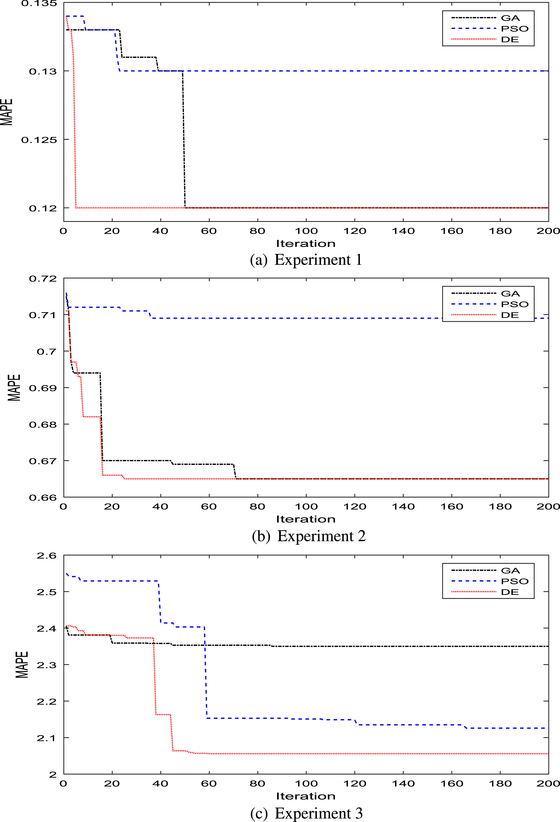
The convergence behavior.

Based on the above results and analyses, it can be initially concluded that the DEABB is more efficient than other conventional and optimization-based methods presented in this paper. However, the results are sometimes very close and are the averages of series of results;.herefore, it is necessary to validate whether the differences between DEABB and the others are significant or not. Therefore, we next perform the paired samples t-test on the forecasting results to get further analyses. Let us set the significance level at 0.1, that is, if the p-value of a test is less than 0.1 then we reject the null hypothesis or the difference is statistically significant. The testing results are presented in Table 3 where the number represents the p-value of the test. The results obtained in Table 3 confirm that the DEABB model outperforms the conventional methods in terms of error prediction. In comparison with other optimization-based methods, such as the GAABB and PSOABB models, the differences are not significant. However, according to their convergence behaviors as analyzed earlier, the DEABB would be the most likely model to reduce the error as well as the computational cost.

Table 3

The results of the paired samples t-test

		Exp. 1	Exp. 2	Exp. 3
Pair 1	AM - DEABB	0.073	0.029	0.675
Pair 2	Chen - DEABB	0.000	0.000	0.001
Pair 3	Huarng - DEABB	0.000	0.000	0.053
Pair 4	GABBB - DEABB	0.356	0.596	0.201
Pair 5	PSOABB - DEABB	0.473	0.813	0.201

4.4 The out-of-sample forecasting

The previous subsection has shown the effectiveness of the DEABB model for in-sample forecasting. We now extend the discussion and conduct the out-of-sample forecasting for the next five years of Vietnam’s GDP and rice production using the DEABB model. It can be implied that the forecasting GDP and rice production of the next five years remain unchanged using the Chen and the Huarng models;.ence both of them are unable to cope with the out-of-sample forecasting. For the DEABB model, as shown in Table 4 new, the forecasting GDP and rice production in the next five years tend to increase substantially. It is possible due to the fact that Vietnam is on the path of development with economic promotion policies. It is evidenced that the DEABB model is a new method which can handle real-world applications in which historical data increase or decrease, continuously.

Table 4
Out-of-sample forecasting results

Year Rice production Year GDP

2015 46157.17 2016 5891.24

2016 47340.09 2017 6119.00

2017 48523.09 2018 6348.12

2018 49706.09 2019 6577.45

2019 50889.09 2020 6807.02

Year	Rice production	Year	GDP
2015	46157.17	2016	5891.24
2016	47340.09	2017	6119.00
2017	48523.09	2018	6348.12
2018	49706.09	2019	6577.45
2019	50889.09	2020	6807.02

5 Conclusion

This paper proposes an improved fuzzy time series model, where the parameters of the AM model are optimized by the differential evolution algorithm. The proposed method can forecast the values that fall outside the min-max range of the original data, whereas most of the previous models are not able to forecast those kinds of values. The illustrative examples confirm the superiority of the DEABB over the conventional methods in terms of the mean of absolute error. In comparison with other optimization-based methods as GAABB and PSOABB, there are no statistically significant differences but the DEABB should be the most reasonable choice due to its ability to quickly reach the global optimum. The proposed model can be applied to numerous practical problems, such as population, GDP, rice production forecasting. The limitation of the proposed method is that it just optimizes the time-invariant fuzzy time series where the intervals have the same length. This has motivated researchers to extend the work towards time-variant AM model and its optimization in the future. Besides, a package can be programmed in R to apply the proposed model as well as other fuzzy time series models to practice.

References

Abbasov

A.M.

, Mamedova

M.H.

, Application of fuzzy time series to population forecasting, in: 8th Symposion on Information Technology in Urban and Spatial Planning, Vienna University of Technology, 2003, pp. 545–552.

Agustin-Blas

L.E.

, Salcedo-Sanz

, Jiménez-Fernández

, Carro-Calvo

, Del Ser

and Portilla-Figueras

J.A.

, A new grouping genetic algorithm for clustering problems, Expert Systems with Applications 39(10) (2012), 9695–9703, ISSN 09574174.

Aladag

C.H.

, Yolcu

, Egrioglu

and Dalar

A.Z.

, A new time invariant fuzzy time series forecasting method based on particle swarm optimization, Applied Soft Computing 12(10) (2012), 3291–3299, ISSN 1568–4946.

Aladag

C.H.

, Egrioglu

, Yolcu

and Uslu

V.R.

, A high order seasonal fuzzy time series model and application to international tourism demand of Turkey, Journal of Intelligent &.uzzy Systems 26(1) (2014), 295–302, ISSN 1064-1246.

Ardia

, Boudt

, Carl

, Mullen

K.M.

and Peterson

B.G.

, Differential evolution with DEoptim, R Journal 3(1) (2011), ISSN 2073–4859.

Bas

, Uslu

V.R.

, Yolcu

and Egrioglu

, A modified genetic algorithm for forecasting fuzzy time series, Applied Intelligence 41(2) (2014), 453–463, ISSN 1573–7497.

Box

G.E.P.

, Jenkins

G.M.

, Time series analysis, Forecasting and control, in: Holden-Day Series in Time Series Analysis, Revised ed., San Francisco: Holden-Day, 1976, (1976).

Chen

S.-M.

, Forecasting enrollments based on fuzzy time series, Fuzzy Sets and Systems 81(3) (1996), 311–319, ISSN 0165-0114.

Chen

S.-M.

, Forecasting enrollments based on high-order fuzzy time series, Cybernetics and Systems 33(1) (2002), 1–16, ISSN 0196-9722.

10.

Chen

S.-M.

and Hsu

C.-C.

, A new method to forecast enrollments using fuzzy time series, International Journal of Applied Science and Engineering 2(3) (2004), 234–244, ISSN 1727-2394.

11.

Cortes

and Vapnik

, Support-vector networks, Machine Learning 20(3) (1995), 273–297, ISSN 0885-6125.

12.

Dacal-Nieto

, Vázquez-Fernández

, Formella

, Martin

, Torres-Guijarro

, González-Jorge

, A genetic algorithm approach for feature selection in potatoes classification by computer vision, 2009, pp. 1955–1960. ISBN 1553-572XVO.

13.

Das

, Abraham

, Konar

, Automatic clustering using an improved differential evolution algorithm, 38 (2008), 218–237. ISBN 1083-4427 VO-38.

14.

De Oliveira

J.F.L.

and Ludermir

T.B.

, A distributed PSOARIMA-SVR hybrid system for time series forecasting, in: Systems, Man and Cybernetics (SMC), 2014 IEEE International Conference on, IEEE, 2014, pp. 3867–3872. ISBN ISBN1479938408.

15.

Durbin

, The fitting of time-series models, Revue de l’Institut International de Statistique 28(3) (1960), 233–244, ISSN 0373-1138.

16.

Engle

R.F.

, Autoregressive conditional heteroscedasticity with estimates of the variance of United Kingdom inflation, Econometrica: Journal of the Econometric Society (1982), 987–1007 ISSN 0012-9682.

17.

Friedman

J.H.

, Multivariate adaptive regression splines, The Annals of Statistics (1991), 1–67, ISSN 0090-5364.

18.

Galton

, Co-relations and their measurement, chiefly from anthropometric data, Proceedings of the Royal Society of London 45(273–279) (1888), 135–145, ISSN 0370-1662.

19.

Garg

, Rani

, Sharma

S.P.

and Vishwakarma

, Intuitionistic fuzzy optimization technique for solving multi-objective reliability optimization problems in interval environment, Expert Systems with Applications 41(7) (2014), 3157–3167, ISSN0957–4174.

20.

Garg

, Solving structural engineering design optimization problems using an artificial bee colony algorithm, Journal of Industrial and Management Optimization 10(3) (2014), 777–794.

21.

Garg

, A hybrid GA-GSA algorithm for optimizing the performance of an industrial system by utilizing uncertain data, in: Handbook of Research on Artificial Intelligence Techniques and Algorithms, IGI Global, 2015, pp. 620–654.

22.

Garg

, An efficient biogeography based optimization algorithm for solving reliability optimization problems, Swarm and Evolutionary Computation 24 (2015), 1–10, ISSN 2210-6502.

23.

Garg

, A hybrid PSO-GA algorithm for constrained optimization problems, Applied Mathematics and Computation 274 (2016), 292–305, ISSN 0096-3003.

24.

Garg

, Performance analysis of an industrial system using soft computing based hybridized technique, Journal of the Brazilian Society of Mechanical Sciences and Engineering 39(4) (2017), 1441–1451, ISSN 1806–3691.

25.

Garg

, Analysis of an industrial system under uncertain environment by using different types of fuzzy numbers, International Journal of System Assurance Engineering and Management 9(2) (2018), 525–538, ISSN 0976-4348.

26.

Ghazali

, Hussain

A.J.

, Al-Jumeily

and Lisboa

, Time series prediction using dynamic ridge polynomial neural networks, in: Developments in eSystems Engineering (DESE), 2009 Second International Conference on, IEEE, 2009, pp. 354–363, ISBN ISBN 1424454026.

27.

Gupta

and Wang

L.P.

, Stock forecasting with feedforward neural networks and gradual data sub-sampling, Australian Journal of Intelligent Information Processing Systems 11(4) (2010), 14–17, ISSN 1321–2133.

28.

Che-Ngoc

, Vo-Van

, Huynh-Le

Q.-C.

, Ho

, Nguyen-Trang

, Chu-Thi

M.-T.

, An Improved Fuzzy Time Series Forecasting Model, in: Econometrics for Financial Applications, Anh

L.H.

, Dong

L.S.

, Kreinovich

and Thach

N.N.

, eds. Springer International Publishing, Cham. 2018. pp. 474–490. ISBN ISBN 978-3-319-73150-6.

29.

Ho-Huu

, Nguyen-Thoi

, Vo-Duy

and Nguyen-Trang

, An adaptive elitist differential evolution for optimization of truss structures with discrete design variables, Computers &.tructures 165 (2016), 59–75, ISSN 0045-7949.

30.

Ho-Huu

, Do-Thi

T.D.

, Dang-Trung

, Vo-Duy

and Nguyen-Thoi

, Optimization of laminated composite plates for maximizing buckling load using improved differential evolution and smoothed finite element method, Composite Structures 146 (2016), 132–147, ISSN 0263-8223.

31.

Holland

J.H.

, Genetic algorithms and the optimal allocation of trials, SIAM Journal on Computing 2(2) (1973), 88–105, ISSN 0097-5397.

32.

Huarng

, Heuristic models of fuzzy time series for forecasting, Fuzzy Sets and Systems 123(3) (2001), 369–386, ISSN 0165-0114.

33.

Huarng

and Yu

H.-K.

, A Type 2 fuzzy time series model for stock index forecasting, Physica A: Statistical Mechanics and its Applications 353 (2005), 445–462, ISSN 0378-4371.

34.

Kachitvichyanukul

, Comparison of three evolutionary algorithms: GA, PSO, and DE, Industrial Engineering and Management Systems 11(3) (2012), 215–223, ISSN 1598–7248.

35.

Kenndy

and Eberhart

R.C.

, Particle swarm optimization, in: Proceedings of IEEE International Conference on Neural Networks, Vol. 4, IEEE Press, 1995, pp. 1942–1948.

36.

Kuo

I.-H.

, Horng

S.-J.

, Kao

T.-W.

, Lin

T.-L.

, Lee

C.-L.

and Pan

, An improved method for forecasting enrollments based on fuzzy time series and particle swarm optimization, Expert Systems with Applications 36(3, Part 2) (2009) 6108–6117, ISSN 0957–4174.

37.

Le-Anh

, Nguyen-Thoi

, Ho-Huu

, Dang-Trung

and Bui-Xuan

, Static and frequency optimization of folded laminated composite plates using an adjusted Differential Evolution algorithm and a smoothed triangular plate element, Composite Structures 127 (2015), 382–394, ISSN 02638223.

38.

Lee

M.H.

and Sadaei

H.J.

, Introducing polynomial fuzzy time series, Journal of Intelligent &.uzzy Systems 25(1) (2013), 117–128, ISSN 1064–1246.

39.

Lewis

P.A.W.

and Stevens

J.G.

, Nonlinear modeling of time series using multivariate adaptive regression splines (MARS), Journal of the American Statistical Association 86(416) (1991), 864–877, ISSN 0162–1459.

40.

Marinoiu

, Forecast of the evolution of employment in romanian agriculture using fuzzy time series, Economic Insights-Trends &.hallenges 68(3) (2016), ISSN 2284-8576.

41.

Park

D.-C.

, A time series data prediction scheme using bilinear recurrent neural network, in: Information Science and Applications (ICISA), 2010 International Conference on, IEEE 2010, pp. 1–7, ISBN ISBN 1424459435.

42.

Patwal

R.S.

, Narang

and Garg

, A novel TVAC-PSO based mutation strategies algorithm for generation scheduling of pumped storage hydrothermal system incorporating solar units, Energy 142 (2018), 822–837, ISSN 0360-5442.

43.

Pearson

, Mathematical contributions to the theory of evolution. III. Regression, heredity, and panmixia, Philosophical Transactions of the Royal Society of London Series A, Containing Papers of a Mathematical or Physical Character 187(1896), 253–318, ISSN 0264–3952.

44.

Price

, Storn

R.M.

and Lampinen

J.A.

, Differential evolution: A practical approach to global optimization, Springer Science &.usiness Media (2006), ISBN ISBN 3540313060.

45.

Qin

A.K.

, Huang

V.L.

and Suganthan

P.N.

, Differential evolution algorithm with strategy adaptation for global numerical optimization, IEEE Transactions on Evolutionary Computation 13(2) (2009), 398–417, ISSN 1089-778X.

46.

Rani

, Gulati

T.R.

and Garg

, Multi-objective non-linear programming problem in intuitionistic fuzzy environment: Optimistic and pessimistic view point, Expert Systems with Applications 64 (2016), 228–238, ISSN 0957–4174.

47.

Ren

, Suganthan

P.N.

, Srikanth

and Amaratunga

, Random vector functional link network for short-term electricity load demand forecasting, Information Sciences 367 (2016) 1078–1093, ISSN 0020–0255.

48.

Sasu

, An application of fuzzy time series to the romanian population, Bulletin of the Transilvania University of Brasov 3 (2010), 52.

49.

Shyi-Ming

and Nien-Yi

, Forecasting enrollments using high-order fuzzy time series and genetic algorithms, International Journal of Intelligent Systems 21(5) (2006), 485–501, ISSN 0884–8173.

50.

Singh

S.R.

, A computational method of forecasting based on fuzzy time series, Mathematics and Computers in Simulation 79(3) (2008), 539–554.

51.

Song

and Chissom

B.S.

, Forecasting enrollments with fuzzy time series part I, Fuzzy Sets and Systems 54(1) (1993), 1–9, ISSN 0165-0114.

52.

Storn

and Price

, Differential evolution âĂŞ. simple and efficient heuristic for global optimization over continuous spaces, Journal of Global Optimization 11(4) (1997), 341–359, ISSN 1573–2916.

53.

Teo

, Wang

and Lin

, Wavelet packet multi-layer perceptron for chaotic time series prediction: Effects of weight initialization, Computational Science-ICCS 2001 (2001), 310–317.

54.

Tseng

F.-M.

and Tzeng

G.-H.

, A fuzzy seasonal ARIMA model for forecasting, Fuzzy Sets and Systems 126(3) (2002), 367–376, ISSN 0165–0114.

55.

Vo-Van

, Nguyen-Thoi

, Vo-Duy

, Ho-Huu

and Nguyen-Trang

, Modified genetic algorithm-based clustering for probability density functions, Journal of Statistical Computation and Simulation 87(10) (2017), 1964–1979. ISSN 0094–9655.

56.

Wang

, Teo

K.K.

and Lin

, Predicting time series with wavelet packet neural networks, in: Neural Networks, 2001 Proceedings IJCNN’01 International Joint Conference on, Vol. 3, IEEE, 2001, pp. 1593–1597, ISBN ISBN0780370449.

57.

Wang

and Fu

, Data mining with computational intelligence, Springer Science &.usiness Media (2006), ISBN ISBN 3540288031.

58.

Wang

, Wu

and Zhao

, Performance comparison of GA, PSO, and DE approaches in estimating low atmospheric refractivity profiles, Wuhan University Journal of Natural Sciences 15(5) (2010), 433–439, ISSN 1993-4998.

59.

H.-K.

, Weighted fuzzy time series models for TAIEX forecasting, Physica A: Statistical Mechanics and its Applications 349(3) (2005), 609–624, ISSN 0378-4371.

60.

Zadeh

L.A.

, Fuzzy sets, Information and Control 8(3) (1965), 338–353, ISSN 0019–9958.

61.

Zecchin

, Facchinetti

, Sparacino

and De

, Nicolao and C. Cobelli, A new neural network approach for short-term glucose prediction using continuous glucose monitoring timeseries and meal information, in: Engineering in Medicine and Biology Society, EMBC, 2011 Annual International Conference of the IEEE, IEEE, 2011, pp. 5653–5656. ISBN ISBN1457715899.

62.

Zhang

G.P.

, Time series forecasting using a hybrid ARIMA and neural network model, Neurocomputing 50 (2003), 159–175, ISSN 0925-2312.

63.

Zhao

and Yang

, PSO-based single multiplicative neuron model for time series prediction, Expert Systems with Applications 36(2, Part 2) (2009), 2805–2812, ISSN 0957-4174.

64.

Zhu

and Wang

, Intelligent trading using support vector regression and multilayer perceptrons optimized with genetic algorithms, in: Neural Networks (IJCNN), The 2010 International Joint Conference on, IEEE, 2010, pp. 1–5. ISBN ISBN142446918X.

An improved fuzzy time series forecasting model using the differential evolution algorithm

Abstract

Keywords

1 Introduction

2.1 The fuzzy time series

2.2 The Abbasov-Mamedova model

3.1 The differential evolution algorithm

4.1 The data sets

4.2 The effects of the parameters F, CR, and maxiter on the optimal solution

Table 4 Out-of-sample forecasting results Year Rice production Year GDP 2015 46157.17 2016 5891.24 2016 47340.09 2017 6119.00 2017 48523.09 2018 6348.12 2018 49706.09 2019 6577.45 2019 50889.09 2020 6807.02

References

Table 4
Out-of-sample forecasting results

Year Rice production Year GDP

2015 46157.17 2016 5891.24

2016 47340.09 2017 6119.00

2017 48523.09 2018 6348.12

2018 49706.09 2019 6577.45

2019 50889.09 2020 6807.02