Estimation and detection of a weak magnetic dipole signal with a latent variable based on a non-probability-distribution EM algorithm

Abstract

The estimation and detection of a weak magnetic dipole signal is a critical problem in magnetic target detection. The difficulty arises due to a latent variable in the model, which affects the estimation and detection performance, especially at low signal-to-noise ratios (SNRs). A non-probability-distribution expectation maximization (NPD-EM) algorithm is proposed to estimate the magnetic dipole signal with the latent variable at low SNRs. A reasonable value of an intermediate variable instead of the optimal one is determined without any probability information in the iteration of the NPD-EM algorithm, which overcomes an unknown probability distribution appearing in the traditional expectation maximization (EM) algorithm and reduces the calculated amount by 3 orders of magnitude compared with the traditional EM algorithm. A statistic based on the NPD-EM algorithm representing an unbiased estimator of the target signal energy is constructed to detect the magnetic dipole signal at low SNRs, and an innovative compensation in the detector is introduced so as to reduce the noise influence on the statistic. The experiment results show that, the constructed detector is comparable to the ideal matching filter due to the attractive performance of the NPD-EM algorithm and the outstanding statistic.

Keywords

EM Algorithm estimation and detection weak magnetic signal latent variable low signal-to-noise ratio

1 Introduction

The estimation and detection of a weak magnetic dipole signal is a critical problem in magnetic target detection, such as pipeline detection, medical micro-apparatus detection and weapon detection [1 –5].

The difficulty occurring in the weak magnetic dipole signal detection arises from a latent variable, especially at low signal-to-noise ratios. The latent variable is a parameter in a detection model that cannot be measured directly. It introduces uncertainty in the detection model and affects the estimation and detection performance especially when the signal-to-noise ratio (SNR) is less than 0 dB. The low SNR is caused by a large detection range or a weak magnetic dipole moment which sometimes may even be reduced manually [6]. At low SNRs, the latent variable is more difficult to process, which makes the estimation and detection performance degraded.

The matching filter is the optimal detector used in time-domain to detect a weak signal [7, 8]. However, the latent variable in the detection model makes the matching functions unclear and affects the detection performance. Traditionally, two kinds of method are applied to solve the problem with a latent variable. One is the method with multi-channel [7]. In these channels, the latent variable would be fixed on different assumed values. Using the matching filters and synthesizing all the channels, the judgment could be done. The advantage of this method is the application of the matching filter which is the optimal detector in time-domain. However, there is a positive correlation between the detection performance and the number of channels. Good performance needs plenty of channels, which might consume lots of hardware resources. The other kind of method is estimating the latent variable at first. Then, the model can be solved based on the estimated value of the latent variable, allowing the statistic of the detector to be built. Common methods applied to the latent variable are the genetic algorithm [8], the neural network algorithm [9, 10], the least squares algorithm [11, 12], et al. The genetic algorithm always needs a great amount of calculation, and some parameters in the algorithm are empirical. The neural network algorithm needs a high SNR which cannot be used in the weak magnetic dipole detection. The least squares algorithm needs a matrix inversion which is nonlinear in the weak magnetic dipole signal problem.

By contrast, the expectation maximization (EM) algorithm is more suitable for the problem with latent variables, which is based on the maximum likelihood theory and requires the posterior probability distribution of the latent variable [13]. However, the probability distribution is unknown in the weak magnetic dipole signal problem.

In this paper, a novel non-probability-distribution (NPD) EM algorithm is proposed to overcome the unknown probability distribution for the estimation and detection of the magnetic dipole signal with the latent variable at low SNRs. First, the weak magnetic dipole detection model is introduced, and the influence of the latent variable in the model estimation and the signal detection is analyzed. Second, the NPD-EM algorithm is proposed to overcome the unknown probability distribution appearing in the traditional EM algorithm and to estimate the signal in the weak magnetic dipole signal problem. Third, a detector is constructed based on the NPD-EM algorithm to detect the weak magnetic dipole signal, in which the statistic represents an unbiased estimator of the target signal energy and an innovative compensation from the NPD-EM algorithm is introduced to reduce the noise influence. Fourth, the feasibility and superiority of the NPD-EM algorithm and constructed detector on the estimation and detection are verified through some experiments with real magnetic target signals and colored noise. Finally, some conclusions are drawn from the related studies.

2 Model of the weak magnetic dipole detection and corresponding latent variable

The detection model of a magnetic target is shown in Fig. 1, where the magnetic target is equivalent to a magnetic dipole. A Cartesian coordinate system is established with the origin at the magnetic dipole. M is the magnetic dipole moment of the dipole. A is the detection path, and a detector observing the magnetic signal magnitude moves along A with speed v which unit is meter per second (m/s). The sampling rate is f_s, and its unit is Hz. The closest proximity approach (CPA) distance is the shortest distance between the magnetic dipole and the detection path, which is indicated by R₀ and the unit is meter (m). The CPA point is the point on the detection path that is closest to the magnetic dipole. In the detection model, the CPA distance R₀ is unmeasurable and is referred to as the latent variable. In the following research, the speed v and the CPA distance R₀ would be unitized; the equivalent f_s is 10 000 Hz. And their units would not be mentioned later.

Fig.1

Detection model of a weak magnetic target.

The observed magnetic dipole signal is indicated by x (n), which is the signal received by the detector shown in Fig. 1. x (n) contains the ideal magnetic dipole signal s (n) and noise w (n). The mathematical model of x (n) can be expressed in Equation (1). $x (n) = s (n) + w (n)$ (1) where n = [-N₀, -N₀ + 1, ... , N₀], and 2N₀ + 1 is the width of sample window. The ideal magnetic dipole signal s (n) is also known as the effective signal or the target signal. From [7, 14], s (n) can be expressed by the unit orthogonal basis functions [f₁ (n) , f₂ (n) , f₃ (n)] as in Equation (2), with any direction of the magnetic dipole moment and any geometric relationship between the magnetic dipole and the detection path.

$s (n) = a_{1} \cdot f_{1} (n) + a_{2} \cdot f_{2} (n) + a_{3} \cdot f_{3} (n)$ (2)

In Equation (2), [a₁, a₂, a₃] are the orthogonal coefficients corresponding to the three unit orthogonal basis functions. And the three unit orthogonal basis functions are expressed in Equation (3). The typical unit orthogonal basis functions are shown in Fig. 2.

Fig.2

Typical unit orthogonal basis functions [f₁ (n), f₂ (n), f₃ (n)]. These functions are built with R₀ = 1, v = 1, f_s = 10000, and N₀ = 60000. n = 0 represents the time the detector reaches the CPA point.

{\begin{matrix} f_{1} (n) = f_{1} (u) |_{u = \frac{vn}{R_{0} f_{s}}} = \sqrt{\frac{128 v}{3 π R_{0} f_{s}}} \frac{u^{2}}{(1 + u^{2})^{5 / 2}} \\ f_{2} (n) = f_{2} (u) |_{u = \frac{vn}{R_{0} f_{s}}} = \sqrt{\frac{128 v}{5 π R_{0} f_{s}}} \frac{u}{(1 + u^{2})^{5 / 2}} \\ f_{3} (n) = f_{3} (u) |_{u = \frac{vn}{R_{0} f_{s}}} \\ = \sqrt{\frac{24 v}{5 π R_{0} f_{s}}} [\frac{1}{(1 + u^{2})^{5 / 2}} - \frac{5}{3} \frac{u^{2}}{(1 + u^{2})^{5 / 2}}] \end{matrix}

(3)

The CPA distance R₀ is the latent variable in the detection model, due to the unmeasurable relative position between the detector and the target. The latent variable R₀ makes the basis functions indeterminate and influences the estimation of the signal model. It can be seen from Equation (3) that the shapes of the unit orthogonal basis functions are associated with the CPA distance R₀, which can affect the amplitude and effective width of the signals. As R₀ increases, the effective width increases and the amplitude decreases. Figure 3 shows the curves of the basis function f₁ (n) at different R₀; f₂ (n) and f₃ (n) are similar to f₁ (n).

Fig.3

Basis functions f₁ (n) with different R₀. The functions are built with f_s = 10000, v = 1, and N₀ = 60000. n = 0 represents the time the detector reaches the CPA point.

The latent variable R₀ has a large influence on the estimation and detection of the magnetic dipole signal. On the one hand, the latent variable R₀ makes the signal model difficult to estimate and the statistic in the detector complex. On the other hand, an inaccurate R₀ reduces the performance of the detector.

For example, the orthogonal coefficients [a₁, a₂, a₃] are the characteristics of the signal model and the basis of the detector. Their values are often calculated by some matching filters with unit orthogonal matching functions [7]. This method is based on the unit orthogonality between the matching functions in the matching filters and the basis functions in the signal model. However, if $R_{0}^{'}$ which is not equal to the true R₀ is used to construct the matching functions $[f_{1}^{'} (n), f_{2}^{'} (n), f_{3}^{'} (n)]$ , the constructed matching functions lose their unit orthogonality with the true basis functions. Therefore, the calculated orthogonal coefficients is not accurate, and the performance of the estimation and detection is degraded.

To ensure the superiority of the estimation and detection performance, the latent variable should be processed appropriately in the estimation and detection of the weak magnetic dipole signal.

3 Estimation of the magnetic dipole signal with the latent variable based on the non-probability-distribution EM algorithm

In this section, the NPD-EM algorithm is proposed based on the traditional EM algorithm to estimate the magnetic dipole signal with the latent variable. First, the traditional EM algorithm applied to this estimation problem is introduced, and the difficulty due to an unknown probability distribution is analyzed. Second, the NPD-EM algorithm is proposed to overcome the difficulty and to estimate the magnetic dipole signal. Third, the feasibility and performance of the NPD-EM algorithm are studied through some numerical experiments and comparison studies.

3.1 Traditional EM algorithm applied to the estimation of the magnetic dipole signal

The traditional EM algorithm applied to the magnetic dipole signal problem is introduced in detail. And the difficulty appearing in the traditional EM algorithm is pointed out, showing the reason why the NPD-EM algorithm is needed.

In the EM algorithm, the unknowns are θ = [a₁, a₂, a₃], the observations are x = [x (- N₀) , x (- N₀ + 1) , . . . , x (N₀)], and the latent variable is R₀. A prior knowledge of the latent variable is R₀ ∈ Φ_R = [r₁, r₂], where r₁ > 0. ${\hat{R}}_{0}^{(t)}$ is the intermediate variable used in step t of the traditional EM algorithm. Assume w (n) is additive white Gaussian noise, and w (n) ∼ N (0, σ²). The log-likelihood function is given in Equation (4).

$\begin{matrix} L_{c} (θ) & = & log p (R_{0}, x | θ) \\ = & log p (x | R_{0}, θ) + log p (R_{0} | θ) \end{matrix}$ (4) where, ${\begin{matrix} P (x | R_{0}, θ) = \prod_{n = - N_{0}}^{N_{0}} \frac{1}{\sqrt{2 π σ}} exp {- \frac{[x (n) - s (n)]^{2}}{2 σ^{2}}} \\ P (R_{0} | θ) = p (R_{0}) = \frac{1}{r_{2} - r_{1}} \end{matrix}$

3.1.1 E-step

Let the estimate of R₀ in step t + 1 be ${\hat{R}}_{0}^{(t + 1)}$ , which is the expectation of R₀ under ${\hat{θ}}^{(t)} = [{\hat{a}}_{1}^{(t)}, {\hat{a}}_{2}^{(t)}, {\hat{a}}_{3}^{(t)}]$ from step t. ${\hat{R}}_{0}^{(t + 1)}$ is expressed in Equation (5). $\begin{matrix} {\hat{R}}_{0}^{(t + 1)} & = & E_{R_{0} | x, {\hat{θ}}^{(t)}} [log p (R_{0}, x | θ)] \\ = & \sum_{R_{0} \in Φ_{R}} [p (R_{0} | x, {\hat{θ}}^{(t)}) \cdot log p (x | R_{0}, θ)] \end{matrix}$ (5) $+ \sum_{R_{0} \in Φ_{R}} [p (R_{0} | x, {\hat{θ}}^{(t)}) \cdot log p (R_{0} | θ)]$

In Equation (5), $p (R_{0} | x, {\hat{θ}}^{(t)})$ is unknown and hard to determine, so ${\hat{R}}_{0}^{(t + 1)}$ cannot be calculated using Equation (5) directly. The standard EM algorithm cannot solve the magnetic dipole signal problem.

Traditionally, the common method to obtain ${\hat{R}}_{0}^{(t + 1)}$ with the unknown $p (R_{0} | x, {\hat{θ}}^{(t)})$ is to convert Equation (5) to a least squares problem. Solving the expectation ${\hat{R}}_{0}^{(t + 1)}$ of the latent variable R₀ under ${\hat{θ}}^{(t)}$ can be equivalent to minimize the mean square error between the observed signal x (n) and the signal $\hat{s} (n) |_{θ = {\hat{θ}}^{(t)}, R_{0} = {\hat{R}}_{0}^{(t + 1)}}$ rebuilt by ${\hat{R}}_{0}^{(t + 1)}$ and ${\hat{θ}}^{(t)}$ . This mean square error is shown in Equation (6). $J = \frac{1}{2 N_{0} + 1} \sum_{n = - N_{0}}^{N_{0}} {[x (n) - \hat{s} (n) |_{θ = {\hat{θ}}^{(t)}, R_{0} = {\hat{R}}_{0}^{(t + 1)}}]}^{2}$ (6)

So, ${\hat{R}}_{0}^{(t + 1)} = arg min_{{\hat{R}}_{0}^{(t + 1)}} J$ (7)

Let $\frac{\partial J}{\partial R_{0}} = 0$ (8)

with ${\begin{matrix} \sum_{n = - N_{0}}^{N_{0}} f_{1} (n) \cdot \frac{\partial f_{2} (n)}{\partial R_{0}} = \sum_{n = - N_{0}}^{N_{0}} f_{2} (n) \cdot \frac{\partial f_{1} (n)}{\partial R_{0}} = 0 \\ \sum_{n = - N_{0}}^{N_{0}} f_{2} (n) \cdot \frac{\partial f_{3} (n)}{\partial R_{0}} = \sum_{n = - N_{0}}^{N_{0}} f_{3} (n) \cdot \frac{\partial f_{2} (n)}{\partial R_{0}} = 0 \\ \sum_{n = - N_{0}}^{N_{0}} f_{1} (n) \cdot \frac{\partial f_{3} (n)}{\partial R_{0}} + \sum_{n = - N_{0}}^{N_{0}} f_{3} (n) \cdot \frac{\partial f_{1} (n)}{\partial R_{0}} = 0 \end{matrix}$ (9)

Then, ${\hat{R}}_{0}^{(t + 1)}$ is the solution of Equation (10), and ${\hat{f}}_{i = 1, 2, 3}^{(t)} (n)$ are the basic functions built by ${\hat{R}}_{0}^{(t)}$ . However, Equation (10) is not easy to solve yet. The unknown probability still troubles the traditional EM algorithm. $\sum_{n = - N_{0}}^{N_{0}} \sum_{i = 1}^{3} {{\hat{a}}_{i}^{(t)} \cdot \frac{\partial {\hat{f}}_{i}^{(t)} (n)}{\partial R_{0}} \cdot [x (n) - {\hat{a}}_{i}^{(t)} \cdot {\hat{f}}_{i}^{(t)} (n)]} = 0$ (10)

3.1.2 M-step

Assuming ${\hat{R}}_{0}^{(t + 1)}$ is obtained, the estimated orthogonal coefficients ${\hat{θ}}^{(t + 1)} = [{\hat{a}}_{1}^{(t + 1)}, {\hat{a}}_{2}^{(t + 1)}, {\hat{a}}_{3}^{(t + 1)}]$ can be determined by maximizing the log-likelihood function with respect to ${\hat{θ}}^{(t + 1)}$ through the partial derivatives shown in Equation (11). $\frac{\partial L_{c} (θ) |_{{\hat{R}}_{0}^{(t + 1)}}}{\partial a_{i}} = 0, i = 1, 2, 3$ (11)

Then, the estimated orthogonal coefficients are shown in Equation (12), and the M-step is finished. ${\hat{a}}_{i}^{(t + 1)} = \sum_{n = - N_{0}}^{N_{0}} x (n) \cdot {\hat{f}}_{i}^{(t + 1)} (n), i = 1, 2, 3$ (12)

3.1.3 Difficulty in the traditional EM algorithm applied to the magnetic dipole signal problem

The difficulty in the traditional EM algorithm applied to the magnetic dipole signal problem is the unknown probability distribution $p (R_{0} | x, {\hat{θ}}^{(t)})$ which results in the difficulty to solve ${\hat{R}}_{0}^{(t + 1)}$ . It makes the standard EM algorithm cannot be realized in the magnetic dipole signal problem. And the common method, replacing the E-step by a least squares problem, solving the unknown probability distribution problem is extremely complex and time-consuming. There is a huge computational cost if the equivalent least squares problem is solved at every step. So the traditional EM algorithm needs to be developed to overcome the difficulty arising from the unknown probability distribution and to guarantee the iteration and the estimation performance.

3.2 Non-probability-distribution EM algorithm

The NPD-EM algorithm is proposed to solve the weak magnetic dipole problem. It overcomes the difficulty appearing in the traditional EM algorithm.

The key idea of the NPD-EM algorithm is to determine an applicable and efficient solution of the intermediate variable without any probability information instead of the optimal solution of the intermediate variable in the traditional EM algorithm to overcome the unknown probability distribution and to guarantee the iteration.

The key idea of the NPD-EM algorithm is based on the theoretical study of the traditional EM algorithm, which is shown in Fig. 4. The NPD-EM algorithm is to maximize the log-likelihood function L_c (θ) by the iteration. In an iteration, such as step t + 1, the traditional EM algorithm constructs an expectation function based on ${\hat{θ}}^{(t)}$ and $L_{c} ({\hat{θ}}^{(t)})$ , then solves ${\hat{θ}}^{(t + 1)}$ by maximizing the expectation function, that is shown in Fig. 4. However, there is an unknown probability distribution in the magnetic dipole signal problem, which makes the expectation function of the traditional EM algorithm cannot be constructed and the iteration fails. As to the NPD-EM algorithm, from Fig. 4, it can be seem that any ${\hat{θ}}^{(t + 1)}$ in $[{\hat{θ}}^{(t)}, {\hat{θ}}_{0}^{(t)}]$ can ensure $L_{c} ({\hat{θ}}^{(t + 1)}) ⩾$ $L_{c} ({\hat{θ}}^{(t)})$ . The ${\hat{θ}}^{(t + 1)}$ in $[{\hat{θ}}^{(t)}, {\hat{θ}}_{0}^{(t)}]$ , may not be the optimal solution in this iteration, but it doesn’t need any probability information and can guarantee the iteration of the NPD-EM algorithm. In other words, the traditional EM algorithm is the optimum in one iteration, but may not be the global optimum and cannot be realized because of an unknown probability distribution; the NPD-EM algorithm is under looser constraint compared with the traditional EM algorithm, which gives up the local iteration optimum but can finish the iteration without any probability information.

Fig.4

The key idea of the NPD-EM algorithm.

The theoretical study of the looser constraint in the NPD-EM algorithm is based on the Jensen’s inequality. The Jensen’s inequality is shown in Equation (13), which means that an expectation of a function is greater than or equal to the function of the expectation. And the traditional EM algorithm is based on the equality of the Jensen’s inequality, the latent variable is estimated when the Jensen’s inequality is equality, which is the optimal solution. While it does not mean that the EM algorithm could not iterate successfully when the Jensen’s inequality is not equal. If there is a Z satisfying Equation (14), the EM method would also iterate successfully. The ${\hat{θ}}^{(t + 1)}$ in the NPD-EM algorithm is the Z satisfying Equation (14). $E [g [(X)] ⩾ g [E (X)]$ (13) $E [g [(X)] ⩾ Z ⩾ g [E (X)]$ (14)

One step in the iteration of the NPD-EM algorithm applied to the weak magnetic dipole signal problem is shown in Fig. 5. Figure 5 also contains the comparison between the traditional EM algorithm and the NPD-EM algorithm. ${\hat{R}}_{0 m}^{(t)}$ is the intermediate variable used in step t of the NPD-EM algorithm, which is corresponding to the latent variable R₀.

Fig.5

One step in the iteration of the NPD-EM algorithm applied to the weak magnetic dipole signal problem, and the comparison between the traditional EM algorithm and the NPD-EM algorithm.

From Fig. 5, it can be seen that, the NPD-EM algorithm applied to the weak magnetic dipole signal problem is to determine the applicable and efficient solution of the intermediate variable ${\hat{R}}_{0 m}^{(t + 1)}$ without any probability information, which includes two aspects: one is how to find ${\hat{R}}_{0 m}^{(t + 1)}$ that is better than ${\hat{R}}_{0 m}^{(t)}$ under ${\hat{θ}}^{(t)}$ , and the other is how to judge whether ${\hat{R}}_{0 m}^{(t + 1)}$ is better than ${\hat{R}}_{0 m}^{(t)}$ . These issues involve the updating problem for ${\hat{R}}_{0 m}^{(t)}$ and will be detailed in the following algorithm parsing. Comparing the traditional EM algorithm and the NPD-EM algorithm applied to the weak magnetic dipole signal problem, the main difference between them is in the E-step. The traditional EM algorithm solves ${\hat{R}}_{0}^{(t + 1)}$ by its expectation under ${\hat{θ}}^{(t)}$ ; the NPD-EM algorithm just finds ${\hat{R}}_{0 m}^{(t + 1)}$ better than ${\hat{R}}_{0 m}^{(t)}$ under ${\hat{θ}}^{(t)}$ .

The NPD-EM algorithm applied to estimate the weak magnetic dipole signal can be divided into four parts: the initialization, the NPD E-step (the update of ${\hat{R}}_{0 m}^{(t)}$ the NPD M-step, and the convergence condition. In the NPD-EM algorithm, there are two instrumental variables $J^{(t)} |_{{\hat{θ}}^{(t)}}$ and $J^{(t + 1)} |_{{\hat{θ}}^{(t)}}$ , expressed in Equations (15) and (16), respectively. The returned values of the NPD-EM algorithm are the estimated model parameters $\hat{θ} = [{\hat{a}}_{1}, {\hat{a}}_{2}, {\hat{a}}_{3}]$ , the estimated latent variable ${\hat{R}}_{0}$ , and the estimated minimum mean square error $\hat{J}$ at the final iteration. The flowchart of the NPD-EM algorithm applied to the weak magnetic dipole signal problem is shown inFig. 6.

Fig.6

The flowchart of the NPD-EM algorithm applied to the weak magnetic dipole signal problem.

$J^{(t)} |_{{\hat{θ}}^{(t)}} = \frac{1}{2 N_{0} + 1} \sum_{n = - N_{0}}^{N_{0}} {[x (n) - \hat{s} (n) |_{θ = {\hat{θ}}^{(t)}, R_{0} = {\hat{R}}_{0 m}^{(t)}}]}^{2}$ (15) $J^{(t + 1)} |_{{\hat{θ}}^{(t)}} = \frac{1}{2 N_{0} + 1} \sum_{n = - N_{0}}^{N_{0}} {[x (n) - \hat{s} (n) |_{θ = {\hat{θ}}^{(t)}, R_{0} = {\hat{R}}_{0 m}^{(t + 1)}}]}^{2}$ (16)

For the initialization, the primary variable is ${\hat{R}}_{0 m}^{(0)}$ which is the initial value of ${\hat{R}}_{0 m}^{(t)}$ corresponding to the latent variable. To ensure the convergence speed of the NPD-EM algorithm, ${\hat{R}}_{0 m}^{(0)}$ needs to be set in [r₁, r₂] according to the prior knowledge of the latent variable R₀ ∈ [r_1,r₂]. Then, ${\hat{θ}}^{(0)}$ and $J^{(0)} |_{{\hat{θ}}^{(0)}}$ can be obtained using Equations (3), (12), and (15).

For the NPD E-step (the update of ${\hat{R}}_{0 m}^{(t)}$ ) the purpose is to determine ${\hat{R}}_{0 m}^{(t + 1)}$ better than ${\hat{R}}_{0 m}^{(t)}$ under ${\hat{θ}}^{(t)}$ , which represents the key idea of the NPD-EM algorithm. A variable increment is employed to update ${\hat{R}}_{0 m}^{(t)}$ and the superiority of ${\hat{R}}_{0 m}^{(t + 1)}$ is judged by the relationship between the two instrumental variables $J^{(t)} |_{{\hat{θ}}^{(t)}}$ and $J^{(t + 1)} |_{{\hat{θ}}^{(t)}}$ . In an iteration, ${\hat{R}}_{0 m}^{(t + 1)}$ can be obtained by Equation (17), where $Δ R_{0}^{(b)}$ is the variable increment and $Δ R_{0}^{(0)}$ depends on the prior knowledge of R₀. If $J^{(t + 1)} |_{{\hat{θ}}^{(t)}} < J^{(t)} |_{{\hat{θ}}^{(t)}}$ , it means that this ${\hat{R}}_{0 m}^{(t + 1)}$ is better than ${\hat{R}}_{0 m}^{(t)}$ under ${\hat{θ}}^{(t)}$ and the NPD E-step in this iteration is finished. If $J^{(t + 1)} |_{{\hat{θ}}^{(t)}} ⩾ J^{(t)} |_{{\hat{θ}}^{(t)}}$ , it means that the absolute value of the variable increment $| Δ R_{0}^{(b)} |$ is too large and the corresponding ${\hat{R}}_{0 m}^{(t + 1)}$ is not suitable. Then, a new variable increment $Δ R_{0}^{(b + 1)}$ updated by Equation (18) is used to calculate a new ${\hat{R}}_{0 m}^{(t + 1)}$ until $J^{(t + 1)} |_{{\hat{θ}}^{(t)}} < J^{(t)} |_{{\hat{θ}}^{(t)}}$ or the convergence condition. Equation (18) is the update of the variable increment, where b₀ is an agreed-upon value which indicates $| Δ R_{0}^{(b)} |$ is small enough ( $Δ R_{0}^{(b)} \to 0)$ when b > b₀. When $J^{(t + 1)} |_{{\hat{θ}}^{(t)}} ⩾ J^{(t)} |_{{\hat{θ}}^{(t)}}$ and b > b₀, $| Δ R_{0}^{(b)} |$ is reduced by a proportionality coefficient k which is in the interval (0,1). When $J^{(t + 1)} |_{{\hat{θ}}^{(t)}} ⩾ J^{(t)} |_{{\hat{θ}}^{(t)}}$ and b > b₀, it means that $| Δ R_{0}^{(b)} |$ is small enough. The variable increment $Δ R_{0}^{(b)}$ should be replaced by its opposite number to guarantee the iteration. At this time, when $Δ R_{0}^{(b)} \to 0^{+}$ indicating ${\hat{R}}_{0 m}^{(t)} > R_{0}$ , $Δ R_{0}^{(b + 1)}$ = $- Δ R_{0}^{(b)}$ can lead to ${\hat{R}}_{0 m}^{(t + 1)} \to R_{0}$ ; when $Δ R_{0}^{(b)} \to 0^{-}$ indicating ${\hat{R}}_{0 m}^{(t)} < R_{0}$ , $Δ R_{0}^{(b + 1)} = - Δ R_{0}^{(b)}$ can lead to ${\hat{R}}_{0 m}^{(t + 1)} \to R_{0}$ .

${\hat{R}}_{0 m}^{(t + 1)} = {\hat{R}}_{0 m}^{(t)} + Δ R_{0}^{(0)} \in (0, r_{2} - r_{1})$ (17) ${\begin{matrix} Δ R_{0}^{(b + 1)} = - Δ R_{0}^{(b)}, \\ when J^{(t + 1)} |_{{\hat{θ}}^{(t)}} > J^{(t)} |_{{\hat{θ}}^{(t)}} and b > b_{0} \\ Δ R_{0}^{(b + 1)} = k \cdot Δ R_{0}^{(b)}, k \in (0, 1) \\ when J^{(t + 1)} |_{{\hat{θ}}^{(t)}} > J^{(t)} |_{{\hat{θ}}^{(t)}} and b ⩽ b_{0} \end{matrix}$ (18)

For the NPD M-step, the purpose is to obtain ${\hat{θ}}^{(t + 1)}$ and $J^{(t + 1)} |_{{\hat{θ}}^{(t + 1)}}$ . ${\hat{θ}}^{(t + 1)}$ is solved using Equation (12), which is same as the M-step in the traditional EM algorithm. Then, $J^{(t + 1)} |_{{\hat{θ}}^{(t + 1)}}$ is solved by Equations (3) and (15) to support the next iteration and the convergence problem.

There are two convergence conditions in the NPD-EM algorithm. One is called the convergence condition of the mean square error. It is about the relationship between the mean square errors $J^{(t)} |_{{\hat{θ}}^{(t)}}$ and $J^{(t + 1)} |_{{\hat{θ}}^{(t + 1)}}$ . When $J^{(t)} |_{{\hat{θ}}^{(t)}} < J^{(t + 1)} |_{{\hat{θ}}^{(t + 1)}}$ , the algorithm is converged. The other is called the convergence condition of the increment. This convergence condition is related to the number of times that the increment is replaced by its opposite number. This number of times is indicated by N_f. If N_f ⩾ N_f0, the algorithm is converged as well, where N_f0 is an agreed-upon value. The convergence condition of the mean square error can guarantee the rapid convergence of the algorithm at ‘ ${\hat{R}}_{0 m}^{(t)} = R_{0}, \exists t$ .’ The convergence condition of the increment can guarantee the rapid convergence of the algorithm at ‘ ${\hat{R}}_{0 m}^{(t)} \neq R_{0}, \forall t$ .’ It should be noted that the convergence condition of the mean square error is also suitable for ‘ ${\hat{R}}_{0 m}^{(t)} \neq R_{0}, \forall t$ .’

3.3 Feasibility and performance of the NPD-EM algorithm

The feasibility and performance of the NPD-EM algorithm are studied through some numerical experiments. The parameters of the magnetic dipole signal detection model and the NPD-EM algorithm are shown in Tables 1 and 2.

Table 1
Parameters of the magnetic dipole signal detection model

Parameters Quantity

Orthogonal coefficients, [a₁, a₂, a₃] [1 , 1]

Speed, v 1

Sampling rate, f_s 10000

Width of sample window, 2N₀ + 1 120001

Range of latent variable, [r₁, r₂] [0.5, 1.5]

Parameters	Quantity
Orthogonal coefficients, [a₁, a₂, a₃]	[1 , 1]
Speed, v	1
Sampling rate, f_s	10000
Width of sample window, 2N₀ + 1	120001
Range of latent variable, [r₁, r₂]	[0.5, 1.5]

Table 2

Parameters of the NPD-EM algorithm

Parameters	Quantity
Initial value of the latent variable, ${\hat{R}}_{0 m}^{(0)}$	0.5
Initial value of the variable increment, $Δ R_{0}^{(0)}$	0.2
Proportionality coefficient, k	0.5
Limit count of b, b₀	10
Limit count of N_f, N_f 0	4

3.3.1 Feasibility of the NPD-EM algorithm

The NPD-EM algorithm is applied to calculate the model parameters $\hat{θ} = [{\hat{a}}_{1}, {\hat{a}}_{2}, {\hat{a}}_{3}]$ and the latent variable ${\hat{R}}_{0}$ when R₀ ∈ [0.5, 1.5]. The solutions of $\hat{θ} = [{\hat{a}}_{1}, {\hat{a}}_{2}, {\hat{a}}_{3}]$ are shown in Fig. 7. The relative errors between the estimated $[{\hat{a}}_{1}, {\hat{a}}_{2}, {\hat{a}}_{3}]$ and the true [a₁, a₂, a₃] are indicated by $e_{{\hat{a}}_{i} | i = 1, 2, 3}$ and are expressed in Equation (19). The relative error between the estimated ${\hat{R}}_{0}$ and the true R₀ is indicated by $e_{{\hat{R}}_{0}}$ and is expressed in Equation (20). $e_{{\hat{R}}_{0}}$ is shown in Fig. 8 when R₀ ∈ [0.5, 1.5].

Fig.7

Estimated model parameters $\hat{θ} = [{\hat{a}}_{1}, {\hat{a}}_{2}, {\hat{a}}_{3}]$ using the NPD-EM algorithm when R₀ ∈ [0 . 5, 1 . 5].

Fig.8

Relative error $e_{{\hat{R}}_{0}}$ between the estimated ${\hat{R}}_{0}$ and the true R₀ when R₀ ∈ [0 . 5, 1 . 5] .

e_{{\hat{a}}_{i}} = ({\hat{a}}_{i} - a_{i}) / a_{i}, i = 1, 2, 3

(19)

e_{{\hat{R}}_{0}} = ({\hat{R}}_{0} - R_{0}) / R_{0}

(20)

Figures 7 and 8 show that, $e_{{\hat{a}}_{i} | i = 1, 2, 3}$ are less than 0.3% and $e_{{\hat{R}}_{0}}$ is less than 0.21% when R₀ ∈ [0.5, 1.5]. That is, the NPD-EM algorithm can accurately estimate the model parameters θ = [a₁, a₂, a₃] and the latent variable R₀.

In addition, Figs. 7 and 8 show that the error in each parameter increases with increasing R₀, because the corresponding effective signal is truncated by the sample window. As R₀ increases, more energy of the effective signal becomes lost. The basis functions of the truncated signal would lose their unit orthogonality by the gradual increase of R₀, which can be seen from $[{\hat{a}}_{1}, {\hat{a}}_{2}, {\hat{a}}_{3}]$ gradually deviating from 1 in Fig. 7. Furthermore, the change in ${\hat{a}}_{2}$ is smaller and smoother than ${\hat{a}}_{1}$ and ${\hat{a}}_{3}$ since f₂ (n) is an odd function; however, f₁ (n) and f₃ (n) are even functions. The orthogonality between f₁ (n) and f₃ (n) would be lost as the signals are truncated, but the orthogonality between f₂ (n) and the other basis functions would not. Increasing the width of sample window can reduce the errors.

The convergence processes of the NPD-EM algorithm are studied through two numerical experiments with different R₀. The convergence processes of these tests are shown in Figs. 9 and 10. The test that assumes R₀ = 1 is called test_R₀=1, and the test that assumes R₀ = 1.07 is called test_R₀=1.07. test_R₀=1 satisfies ‘ ${\hat{R}}_{0 m}^{(t)} = R_{0,} \exists t$ ’ and would meet the convergence condition of the mean square error. test_R₀=1.07 satisfies ‘ ${\hat{R}}_{0 m}^{(t)} \neq R_{0}, \forall t$ ’ and would meet the convergence condition of the increment.

Fig.9

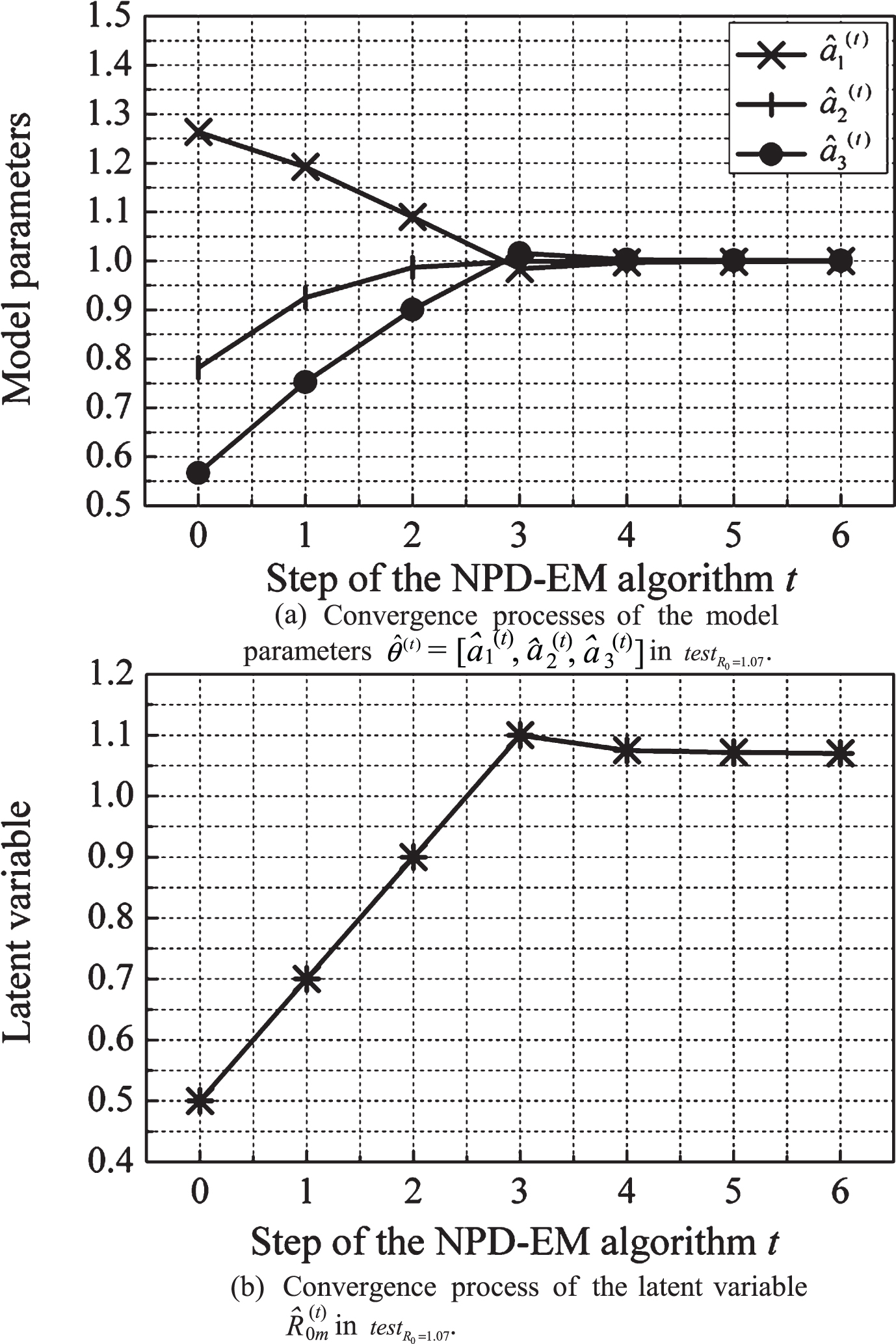
Convergence process of test_R₀=1 with R₀ = 1. test_R₀=1 satisfies ‘ ${\hat{R}}_{0 m}^{(t)} = R_{0}, | \exists t$ ’ and meets the convergence condition of the mean square error.

Fig.10

Convergence process of test_R₀=1.07 with R₀ = 1.07. test_R₀=1.07 satisfies ‘ ${\hat{R}}_{0 m}^{(t)} \neq R_{0}, \forall t$ ’ and meets the convergence condition of the increment.

In test_R₀=1, Fig. 9 shows that there are three iterative times for the NPD-EM algorithm. The variable increments in the iteration process are [0.2, 0.2, 0.1]. ${\hat{R}}_{0 m}^{(t)}$ accurately converges to the true value 1. ${\hat{θ}}^{(t)} = [a_{1}^{(t)}, a_{2}^{(t)}, a_{3}^{(t)}]$ converge to [0.9996, 1.0000, 1.0003] and the maximum $e_{{\hat{a}}_{i} | i = 1, 2, 3}$ is only 0.04%.

In test_R₀=1.07, Fig. 10 shows that there are six iterative times for the NPD-EM algorithm. The variable increments in the iteration process are [0.2, 0.2, 0.2, - 0.2 × 2^-3, - 0.2 × 2^-6, - 0.2 × 2^-7]. ${\hat{R}}_{0 m}^{(t)}$ converges to 1.0731, and $e_{{\hat{R}}_{0}}$ is only 0.29%. ${\hat{θ}}^{(t)} = [a_{1}^{(t)}, a_{2}^{(t)}, a_{3}^{(t)}]$ converge to [0.9994, 1.0000, 1.0004] so that the maximum $e_{{\hat{a}}_{i} | i = 1, 2, 3}$ is only 0.06%. In the third iteration, the condition to replace the variable increment with its opposite number is satisfied. At this time, ${\hat{R}}_{0 m}^{(3)} = 1.1 > R_{0}$ . There is no ${\hat{R}}_{0 m}^{(4)} = {\hat{R}}_{0 m}^{(3)} + Δ R_{0}^{(b)}$ satisfying $J^{(4)} |_{{\hat{θ}}^{(3)}} < J^{(3)} |_{{\hat{θ}}^{(3)}}$ when $Δ R_{0}^{(b)} > 0$ . So, the variable increment should be replaced by its opposite number, then ${\hat{R}}_{0 m}^{(4)} < {\hat{R}}_{0 m}^{(3)}$ and ${\hat{R}}_{0 m}^{(t)}$ tends to the true value.

From Figs. 9 and 10, it can be seen that test_R₀=1.07 is almost converged by the third iteration when test_R₀=1 converges. In test_R₀=1.07, ${\hat{θ}}^{(3)} = [{\hat{a}}_{1}^{(3)}, {\hat{a}}_{2}^{(3)}, {\hat{a}}_{3}^{(3)}]$ is [0.9840, 1.0000, 1.0156] and the maximum corresponding $e_{{\hat{a}}_{i} | i = 1, 2, 3}$ is only 1.56%; ${\hat{R}}_{0 m}^{(3)}$ is 1.1 and the corresponding $e_{{\hat{R}}_{0}}$ test_R₀=1 2.8%. These results are acceptable for some occasions when the accuracy requirement is not very strict. Therefore, the iterative times for the NPD-EM algorithm can be reduced according to the accuracy requirement. The least iteration times and the precision are determined by R₀, ${\hat{R}}_{0 m}^{(0)}$ , Δ $R_{0}^{(0)}, k, b_{0}, and [r_{1}, r_{2}]$ together.

3.3.2 Comparison between the NPD-EM algorithm and the traditional EM algorithm

In the magnetic dipole signal problem, the standard EM algorithm cannot be applied because of the unknown probability distribution. So, the comparison study is between the NPD-EM algorithm and the traditional EM algorithm in which the E-step is replaced by a least squares problem.

To compare the two EM algorithms, the problems in test_R₀=1 and test_R₀=1.07 are also solved by the traditional EM algorithm in which the E-step is replaced by a least squares problem. Equation (10) in the equivalent least squares problem of the traditional EM algorithm is solved by Newton method which is a typical numerical method to solve equations. Then the results of the two algorithms are compared in Table 3.

Table 3
The comparison between the NPD-EM algorithm and the traditional EM algorithm in which the E-step is replaced by a least squares problem

Parameters NPD-EM Traditional EM

test _R₀=1 test _R₀=1.07 test _R₀=1 test _R₁=1.07

Estimated [a₁, a₂, a₃] [0.9996, 1.0000, 1.0003] [0.9994, 1.0000, 1.0004] [0.9988, 1.0000, 1.0011] [0.9982, 1.0000, 1.0016]

Estimated R₀ 1.0000 1.0731 1.0017 1.0726

Iterative times 3 6 8 8

Elapsed time 0.35s 0.71s 1528s 1599s

Parameters	NPD-EM	Traditional EM
Estimated [a₁, a₂, a₃]	[0.9996, 1.0000, 1.0003]	[0.9994, 1.0000, 1.0004]	[0.9988, 1.0000, 1.0011]	[0.9982, 1.0000, 1.0016]
Estimated R₀	1.0000	1.0731	1.0017	1.0726
Iterative times	3	6	8	8
Elapsed time	0.35s	0.71s	1528s	1599s

In Table 3, the most attractive comparison between the two algorithms is the elapsed time. The elapsed time of the NPD-EM algorithm is 3 orders of magnitude less than the elapsed time of the traditional EM algorithm, which shows that the calculated amount of the NPD-EM algorithm is much smaller than the calculated amount of the traditional EM algorithm. The big difference on the calculated amount between the two algorithms is because of the different E-step. In each step, the NPD-EM algorithm just finds an applicable and efficient solution of the intermediate variable by a simple way with little calculated amount; the traditional EM algorithm calculates the intermediate variable by solving Equation (10) with a numerical method causing huge calculated amount.

As to the iterative times, the NPD-EM algorithm is less than the traditional EM algorithm. It proves that the traditional EM algorithm or the standard EM algorithm may be the optimum in each step, but they may not be the global optimum. The NPD-EM algorithm with less iterative times are more efficient than the traditional EM algorithm or the standard EM algorithm in the completed iterative process.

As to the precision of the estimation, the two algorithms are both accurate. All of the relative errors in estimation are less than 0.3%. The less calculated amount in the NPD-EM algorithm does not influence the accuracy of the algorithm.

From the comparison study, it shows that the NPD-EM algorithm can solve the magnetic dipole signal problem accurately and more efficient, while the standard EM algorithm cannot solve because of an unknown probability distribution and the traditional EM algorithm needs huge calculated amount.

3.3.3 Estimation performance of the NPD-EM algorithm in the presence of noise

To study the estimation performance of the NPD-EM algorithm in the presence of noise, the signal expressed in Equation (1) is employed, and the Monte-Carlo simulation is applied. The SNR indicated by SNR is expressed in Equation (21). There are 5000 Monte-Carlo simulation times for each SNR. The results about the estimation performance of the NPD-EM algorithm are shown inTable 4.

In Table 4, the expectations and variances of the estimated model parameters [a₁, a₂, a₃] and latent variable ${\hat{R}}_{0}$ at different SNRs are shown. $e_{\hat{s}}$ expressed in Equation (22) is the relative error between the target signal s (n) and the estimated signal $\hat{s} (n)$ , where $\hat{s} (n)$ is rebuilt by the estimated model parameters $[{\hat{a}}_{1,} {\hat{a}}_{2,} {\hat{a}}_{3}]$ and latent variable ${\hat{R}}_{0}$ . The mean values of $e_{\hat{s}}$ at different SNRs are also shown in Table 4 to verify the estimation accuracy on the signal.

Table 4
The Monte-Carlo simulation results about the estimation performance of the NPD-EM algorithm at different SNRs

SNR ${\hat{a}}_{1}$ ${\hat{a}}_{2}$ ${\hat{a}}_{3}$ ${\hat{R}}_{0}$ $e_{\hat{s}}$

Expectation Variance Expectation Variance Expectation Variance Expectation Variance Mean

α 1 0 1 0 1 0 1 0 0

0 dB 0.9997 2 . 34 × 10^-5 1.0002 2 . 53 × 10^-5 1.0002 3 . 43 × 10^-5 1.0002 2 . 86 × 10^-5 0.003%

-10 dB 0.9994 2 . 34 × 10^-4 0.9999 2 . 47 × 10^-4 1.0001 3 . 37 × 10^-4 1.0003 2 . 86 × 10^-4 0.030 %

-20 dB 0.9988 2 . 28 × 10^-3 1.0007 2 . 50 × 10^-3 1.0002 3 . 43 × 10^-3 1.0020 2 . 78 × 10^-3 0.312 %

-30 dB 0.9969 2 . 58 × 10^-2 1.0137 2 . 55 × 10^-2 0.9908 3 . 64 × 10^-2 1.0137 3 . 47 × 10^-2 3.117 %

-34 dB 1.0053 6 . 42 × 10^-2 1.0336 6 . 48 × 10^-2 0.9644 9 . 66 × 10^-2 1.0146 9 . 79 × 10^-2 8.182 %

-40 dB 1.0994 2 . 50 × 10^-1 1.0712 3 . 50 × 10^-1 0.8108 4 . 01 × 10^-1 0.9650 3 . 88 × 10^-1 36.84 %

SNR	${\hat{a}}_{1}$	${\hat{a}}_{2}$	${\hat{a}}_{3}$	${\hat{R}}_{0}$	$e_{\hat{s}}$
α	1	0	1	0	1	0	1	0	0
0 dB	0.9997	2 . 34 × 10^-5	1.0002	2 . 53 × 10^-5	1.0002	3 . 43 × 10^-5	1.0002	2 . 86 × 10^-5	0.003%
-10 dB	0.9994	2 . 34 × 10^-4	0.9999	2 . 47 × 10^-4	1.0001	3 . 37 × 10^-4	1.0003	2 . 86 × 10^-4	0.030 %
-20 dB	0.9988	2 . 28 × 10^-3	1.0007	2 . 50 × 10^-3	1.0002	3 . 43 × 10^-3	1.0020	2 . 78 × 10^-3	0.312 %
-30 dB	0.9969	2 . 58 × 10^-2	1.0137	2 . 55 × 10^-2	0.9908	3 . 64 × 10^-2	1.0137	3 . 47 × 10^-2	3.117 %
-34 dB	1.0053	6 . 42 × 10^-2	1.0336	6 . 48 × 10^-2	0.9644	9 . 66 × 10^-2	1.0146	9 . 79 × 10^-2	8.182 %
-40 dB	1.0994	2 . 50 × 10^-1	1.0712	3 . 50 × 10^-1	0.8108	4 . 01 × 10^-1	0.9650	3 . 88 × 10^-1	36.84 %

SNR = 10 \cdot {log}_{10} \frac{\sum_{n = - N_{0}}^{N_{0}} {[s (n)]}^{2}}{(2 N_{0} + 1) σ^{2}}

(21)

e_{\hat{s}} = \frac{\sum_{n = - N_{0}}^{N_{0}} {[s (n) - \hat{s} (n)]}^{2}}{\sum_{n = - N_{0}}^{N_{0}} {[s (n)]}^{2}}

(22)

From Table 4, it can be seen that the expectations of the estimated model parameters $[{\hat{a}}_{1,} {\hat{a}}_{2,} {\hat{a}}_{3}]$ and latent variable ${\hat{R}}_{0}$ are always around the true value 1, while the variances and the mean of $e_{\hat{s}}$ increase with a decrease in SNR. When SNR≥-30 dB, the deviations between the expectations and the true values are less than 1.4% of the corresponding true values, the maximum variance is only 3.64% of the corresponding true value, and the maximum mean of $e_{\hat{s}}$ is only 3.117%. When SNR ⩾ -34dB,, the deviations between the expectations and the true values are less than 4% of the corresponding true values, the maximum variance is only 9.79% of the corresponding true value, and the mean of $e_{\hat{s}}$ is only 8.182%. When SNR =- 40 dB, the deviations between the expectations and the true values are less than 19% of the corresponding true values, the maximum variance is 40.1% of the corresponding true value, and the mean of $e_{\hat{s}}$ is 36.84%. Thus, when SNR≥-34 dB, the performance of the NPD-EM algorithm is satisfied.

Therefore, the NPD-EM algorithm is reasonable and feasible for estimating the signal model, especially processing the latent variable. The estimation precision of the NPD-EM algorithm is attractive in noise-free signals, and the estimation performance of the NPD-EM algorithm in noisy signals is satisfied when SNR ≥-34 dB. These characteristics are suitable for the estimation and detection of the weak magnetic dipole signal with the latent variable.

4 Detection of the weak magnetic dipole signal based on the non-probability-distribution EM algorithm

In this section, a detector based on the NPD-EM algorithm is constructed to detect the weak magnetic dipole signal. The statistic in the detector represents an unbiased estimator of the target signal energy, and an innovative compensation from the NPD-EM algorithm is introduced to reduce the noise influence. The performance of the detector is studied and is compared with an ideal matching filter.

4.1 Construction of the detector based on the NPD-EM algorithm

A detector can be built according to Equation (23), for which the corresponding statistic is T. Thus, this detector is called the detector T. Based on the energy of the effective signal s (n), the statistic T is built with both the convergence characteristics of the NPD-EM algorithm and the relationship between the NPD-EM algorithm and the corresponding ideal matching filter. ${\begin{matrix} H_{0} : T < λ \\ H_{1} : T ⩾ λ \end{matrix}$ (23)

In Equation (23), H₀ represents that there is no magnetic dipole signal in the observation, H₁ represents that there is a magnetic dipole signal in the observation, and λ is a threshold. The expression of the statistic T is given in Equation (24), where $\hat{J}$ is the estimated mean square error and $[{\hat{a}}_{1}, {\hat{a}}_{2}, {\hat{a}}_{3}]$ are the estimated orthogonal coefficients from the NPD-EM algorithm. The energy of the effective signal s(n) is indicated by En and is expressed in Equation (25). $T = {\hat{a}}_{1}^{2} + {\hat{a}}_{2}^{2} + {\hat{a}}_{3}^{2} - 3 \hat{J}$ (24) $En = a_{1}^{2} + a_{2}^{2} + a_{3}^{2}$ (25)

The statistic T can be regarded as the unbiased estimator of En, due to the innovative compensation $- 3 \hat{J}$ from the NPD-EM algorithm. To analyze the expression of the statistic T and the compensation $- 3 \hat{J}$ , the relationship between the NPD-EM algorithm and the corresponding ideal matching filter is studied.

In the corresponding ideal matching filter, the latent variable R₀ and the unit orthogonal basis functions [f₁ (n) , f₂ (n) , f₃ (n)] are known. Thus, the estimators of θ = [a₁, a₂, a₃] by the ideal matching filter can be expressed in Equation (26). With the noise w(n), the estimators $[{\hat{a}}_{1 M}^{2}, {\hat{a}}_{2 M}^{2}, {\hat{a}}_{3 M}^{2}]$ are biased and their expectations are $E = a_{i}^{2} |_{i = 1, 2, 3} + σ^{2}$ , where σ² is the variance of the noise and needs to be compensated for unbiased estimation. Therefore, the unbiased estimator of En by the ideal matching filter is indicated by T_M and is expressed in Equation (27), where the expectation of T_M is E [T_M] = En . ${\hat{a}}_{iM} |_{i = 1, 2, 3} = \sum_{n = - N_{0}}^{N_{0}} x (n) \cdot f_{i = 1, 2, 3} (n)$ (26) $T_{M} = {\hat{a}}_{1 M}^{2} + {\hat{a}}_{2 M}^{2} + {\hat{a}}_{3 M}^{2} - 3 σ^{2}$ (27)

In the NPD-EM algorithm, estimating θ = [a₁, a₂, a₃] is a process of gradually approaching the corresponding ideal matching filter. On the one hand, when the NPD-EM algorithm is converged, ${\hat{R}}_{0 m} \to R_{0}$ and ${\hat{f}}_{i = 1, 2, 3} (n) \to f_{i = 1, 2, 3} (n)$ . Thus, Equation (12) is equivalent to Equation (26) and ${\hat{a}}_{i}^{2} | i = 1, 2, 3 \to {\hat{a}}_{iM}^{2} | i = 1, 2, 3$ . On the other hand, the optimum solution of the latent variable R₀ is based on the minimum mean square error between the observed signal and the estimated signal. When the NPD-EM algorithm is converged, the mean square error is minimum, then $\hat{s} (n) \to s (n)$ . At this time, the mean square error $\hat{J}$ is expressed in Equation (28), which shows that $\hat{J}$ can replace σ² to compensate the deviation from the noise.

Therefore, replacing ${\hat{a}}_{iM}^{2} |_{i = 1, 2, 3}$ and σ² in Equation (27) with ${\hat{a}}_{i}^{2} |_{i = 1, 2, 3}$ and $\hat{J}$ respectively, the statistic T can be expressed in Equation (24). Thus, the statistic T represents the unbiased estimator of En, and the innovative compensation $- 3 \hat{J}$ from the NPD-EM algorithm is used to reduce the deviation from the noise. Because of this, the expectation of the statistic T is hardly influenced by the noise intensity. $\begin{matrix} \hat{J} = {\sum_{n = - N_{0}}^{N_{0}} {[x (n) - \hat{s} (n)]}^{2}} / - (2 N_{0} + 1) \\ = {\sum_{n = - N_{0}}^{N_{0}} {[s (n) - \hat{s} (n) + w (n)]}^{2}} / - (2 N_{0} + 1) \\ = {\sum_{n = - N_{0}}^{N_{0}} {[w (n)]}^{2}} / - (2 N_{0} + 1) = σ^{2} \end{matrix}$ (28)

Besides, the statistic T with a clear physical meaning is helpful for calculating other auxiliary parameters. An example is the SNR of the sampled signal, which can be estimated using Equation (29). $\hat{SNR} = 10 \cdot {log}_{10} (T / \hat{J})$ (29)

4.2 Detection performance

To verify the outstanding performance of the detector T based on the NPD-EM algorithm, the detector is studied at different SNRs using Monte-Carlo simulations with additive white Gaussian noise. The parameters of the detection model and the NPD-EM algorithm are shown in Table 1 and 2. Besides, R₀ = 1 and there are 5000 Monte-Carlo simulation times for each SNR. Thus, the receiver operating characteristic (ROC) curves of the detector T are shown in Fig. 11, where P_D is the detection probability and P_FA is the false alarm probability.

Fig.11

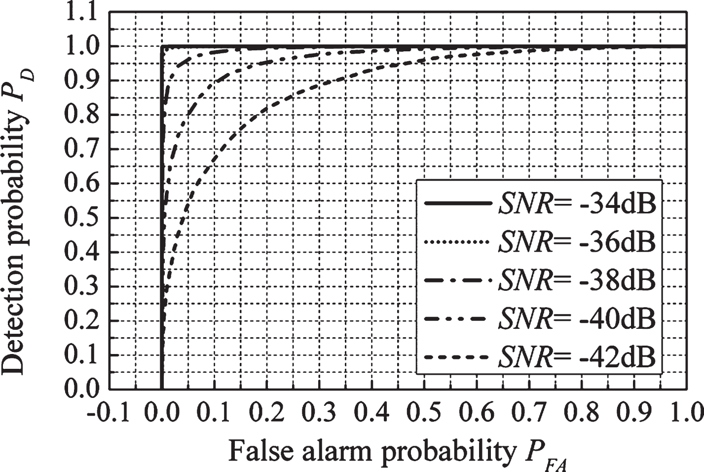
ROC curves of the detector T at different SNRs.

From Fig. 11, it can be seen that the detection performance worsens when the SNR decreases. When SNR = -34 dB, the ROC curve is an ideal curve, in which P_FA = 0 and P_D = 1 Thus, when SNR ⩾ -34dB, the detector T can be regarded as an ideal detector. Assuming P_FA = 0.01 , P_D = 0.09 and P_D = 0.87 when SNR = -36dB and SNR = -38dB, respectively. Assuming P_FA = 0.05, P_D = 0.96 and P_D = 0.8 when SNR = -38dB and SNR = -40dB, respectively.

To study the performance limit of the detector T based on the NPD-EM algorithm, its relationship with the ideal matching filter should be studied. The matching filter, which is also called the correlation detector, performs optimally in time-domain detection. In the ideal matching filter, the unit orthogonal basis functions [f₁ (n) , f₂ (n) , f₃ (n)], the latent variable R₀ and the noise variance σ² are known. T_M expressed in Equation (27), which is the unbiased estimator of En, is employed as the statistic in the ideal matching filter to correspond with the statistic T based on the NPD-EM algorithm. The ideal matching filter based on the statistic T_M is called the detector T_M. Comparing the statistics T_M and T, the relationship between the variances of T_M and T is Var[T] ≥ Var[T_M], because the latent variable R₀ and the unit orthogonal basis functions [f₁ (n) , f₂ (n) , f₃ (n)] need to be estimated in the NPD-EM algorithm. When the estimation of the latent variable R₀ and the basis functions [f₁ (n) , f₂ (n) , f₃ (n)], is accurate enough in the NPD-EM algorithm, the detector T can be equivalent to the detector T_M. That is, the performance of the detector T_M based on the ideal matching filter is the performance limit of the detector T based on the NPD-EM algorithm. Figure 12 shows the relationship between the detector T and the performance limit.

Fig.12

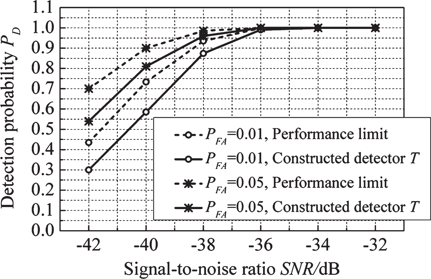
Comparison between the detector T and the performance limit. The detector T is based on the NPD-EM algorithm with the latent variable unknown. The performance limit is based on the ideal matching filter T_M with the latent variable R₀ known.

From Fig. 12, it can be seen that the difference between the performance limit and the performance of the detector T based on the NPD-EM algorithm decreases with increasing SNR. When SNR ⩾ -38dB, there are still gaps between the performance limit and the performance of the detector T. When SNR ⩾ -36dB, the gaps are very small. When SNR ⩾ ; -34dB, the performance of detector T achieves the performance limit. This is because, when SNR ⩾ -34dB, the NPD-EM algorithm estimates the latent variable R₀ and the model parameters θ = [a₁, a₂, a₃] accurately enough, which can be seen in Table 4. That is, because of the accurate estimation of the NPD-EM algorithm when SNR ⩾ -34dB, the performance of the detector T based on the NPD-EM algorithm is comparable with an ideal matching filter.

Above all, the performance of detector T based on the NPD-EM algorithm is perfect when SNR ⩾ -34dB and is acceptable when SNR ⩾ -40dB. One more important note: when SNR ⩾ - 34dB, the performance of the detector T based on the NPD-EM algorithm is comparable with an ideal matching filter and is no longer affected by the latent variable, due to the excellent performance of the NPD-EM algorithm.

5 Experiments on the estimation and detection with real magnetic target signals and noise

By some experiments in a magnetic detection system with real magnetic target signals and colored noise, the superiority and feasibility of the NPD-EM algorithm and the constructed detector T are verified.

In the experiment system, the relative position between the detector and the magnetic target is shown in Fig. 1. The detector is constructed by a fluxgate sensor ‘Mag03’, a signal acquisition ‘NI USB-4432’, and a PC. The sampling rate is f_s = 10000Hz. The width of sample window is 2N₀ + 1 = 120001. The relative speed between the detector and the magnetic target is v = 1m/s . The real CPA distance is R₀ = 1m. The frequency-domain characteristic of the noise in the experiment field is shown in Fig. 13. It can be seen that the noise is colored. Its energy is mainly concentrated in low frequency bands. And the DC offset in the noise is from the geomagnetic field.

Fig.13

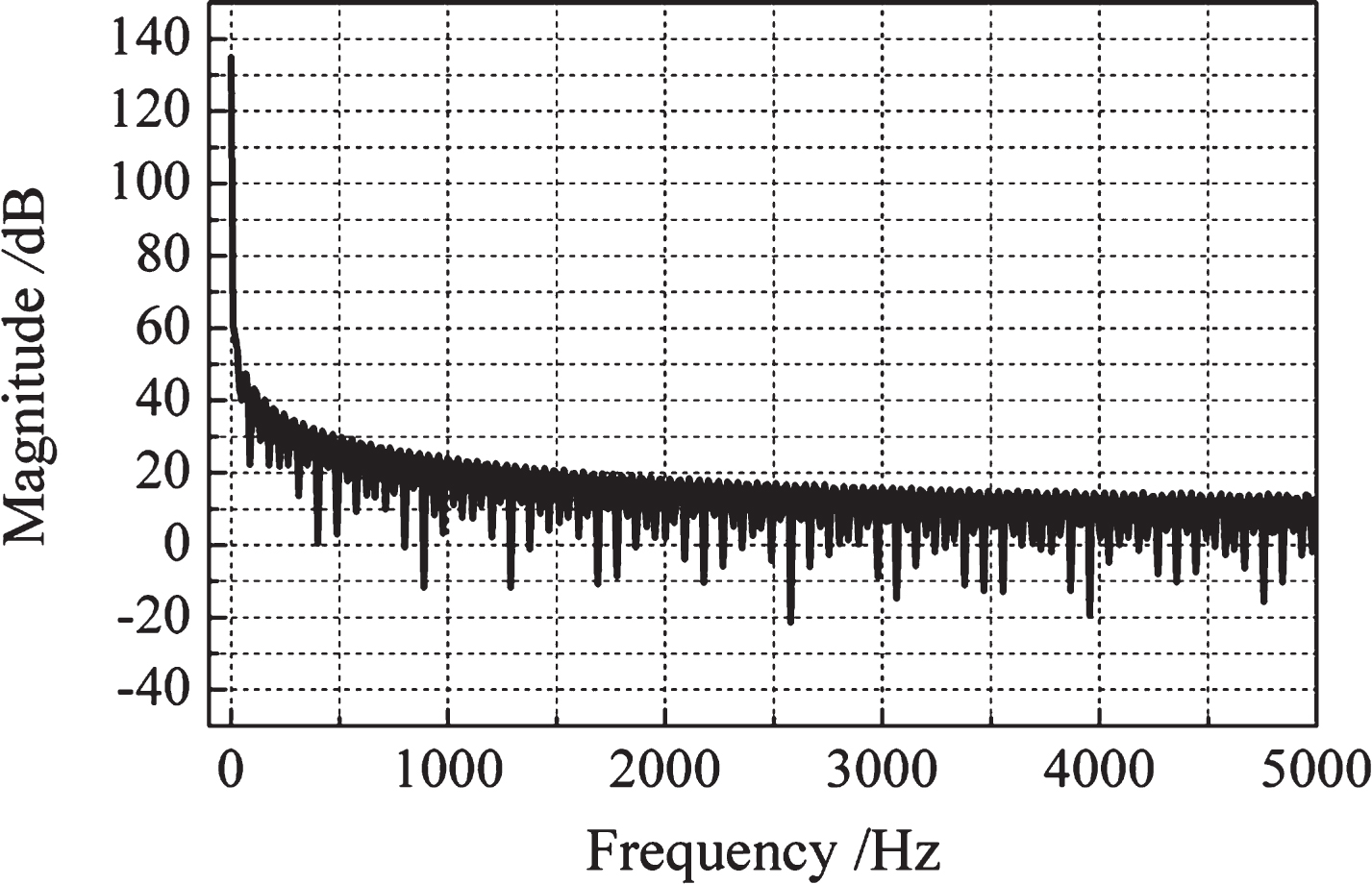
Frequency-domain characteristic of the noise in experiments.

Besides, a low pass filter (LPF), which is a finite impulse response filter with the cut-off frequency being 1 Hz, can be employed to preprocess the observed signals. The estimation and detection results with and without the LPF are compared and analyzed.

5.1 Estimation of the real magnetic target signal by the NPD-EM algorithm

The NPD-EM algorithm is employed to estimate the real magnetic target signal. Real magnetic target signals and the corresponding estimated signals are compared in Fig. 14. The estimation results with and without the LPF are shown in Fig. 14 andTable 5.

Fig.14

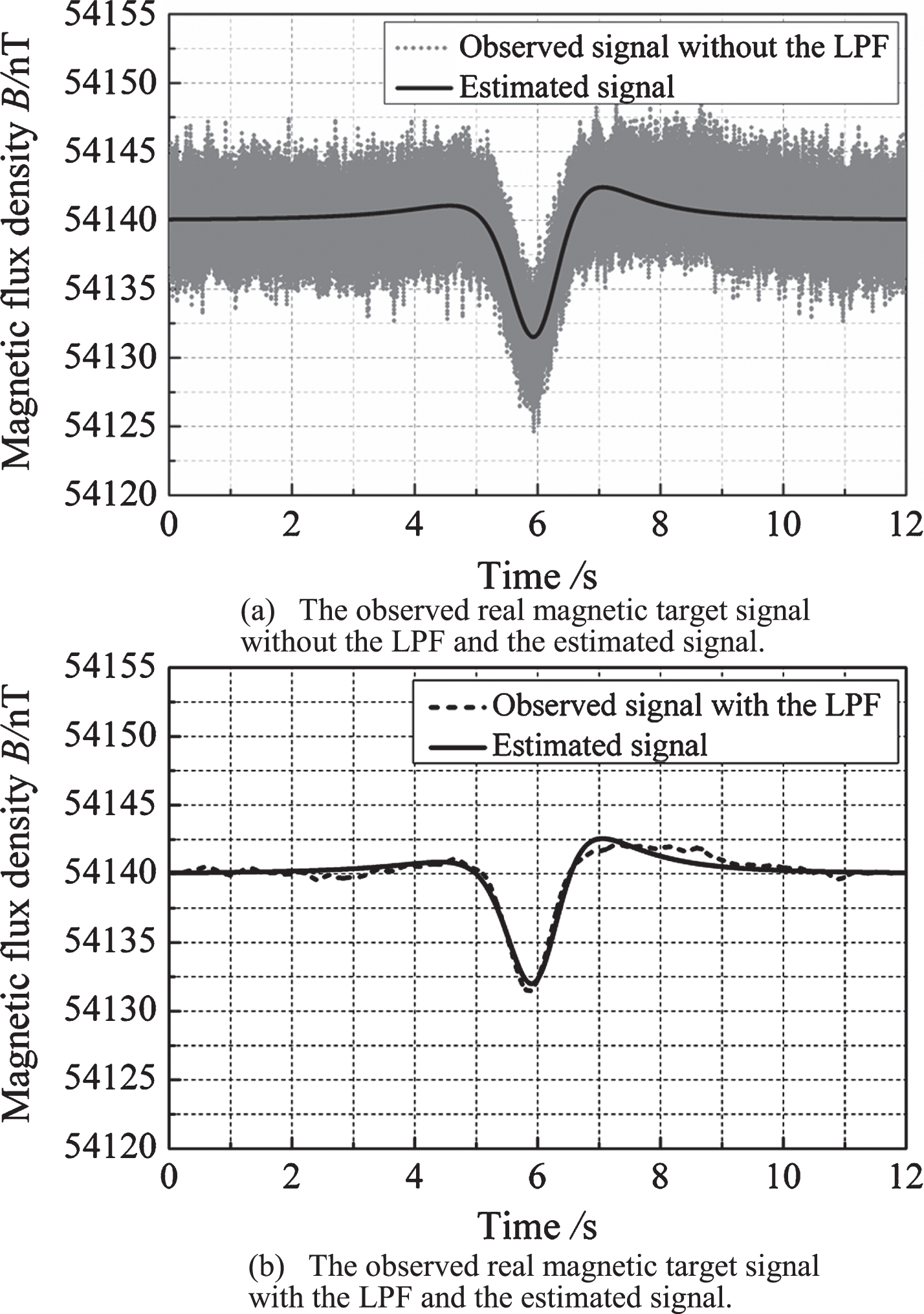
Comparison between the observed real magnetic target signals and the estimated signals.

Table 5

Estimated parameters by the NPD-EM algorithm from the real magnetic target signals in the experiment

Signal	${\hat{a}}_{1} / 1 0^{- 2}$	${\hat{a}}_{2} / 1 0^{- 2}$	${\hat{a}}_{3} / 1 0^{- 2}$	${\hat{R}}_{0} / m$
Without LPF	0.68	1.91	– 6.67	0.9910
With LPF	0.68	2.47	– 6.30	1.0344

In Fig. 14(a), the estimated signal shows the main characteristic of the observed signal without the LPF. In Fig. 14(b), the estimated signal and the observed signal with the LPF are exactly similar. Using Equation (30), the estimated relative error e_est is 4.59%, where x_lpf (n) is the observed signal with the LPF and $\hat{s} (n)$ is the estimated signal. Comparing the estimation results with and without the LPF, there are some differences in the estimated parameters $[{\hat{a}}_{1}, {\hat{a}}_{2}, {\hat{a}}_{3}]$ , but the estimated values of the latent variable ${\hat{R}}_{0}$ are both close to the real CPA distance R₀ = 1. The maximum error of the ${\hat{R}}_{0}$ is only 3.44% of the real CPA distance. That is, the NPD-EM algorithm can estimate the real magnetic target signal in noisy signals, especially the latent variable CPA distance R₀.

From Table 5, it can be seen that the LPF still has some influences on the estimation. The estimated latent variable ${\hat{R}}_{0}$ without the LPF is smaller and more accurate than the estimated latent variable ${\hat{R}}_{0}$ with the LPF, due to the smoothing of the LPF. Thus, the LPF would impact the estimation performance and is not recommended. $e_{est} = \frac{\sum_{n = - N_{0}}^{N_{0}} {[x_{lpf} (n) - \hat{s} (n)]}^{2}}{\sum_{n = - N_{0}}^{N_{0}} {[\hat{s} (n)]}^{2}}$ (30)

5.2 Detection of the weak real magnetic target signal by the detector T

In this experiment, the detector T based on the NPD-EM algorithm is employed to detect the real magnetic target signal at the low SNR, which verifies the superiority of the detector T. The experiment results with and without the LPF are both shown in Fig. 15 and Table 6. In the experiment, the detector reached the CPA point at the 34th second. The time scale of the statistic is set as the middle of the corresponding sample window. Thus, the time the statistic peaks can be regarded as the time the detector reaches the CPA point. The time the statistic peaks is indicated by t₀, and the estimated results at t₀ are also shown in Fig. 15 and Table 6.

Fig.15

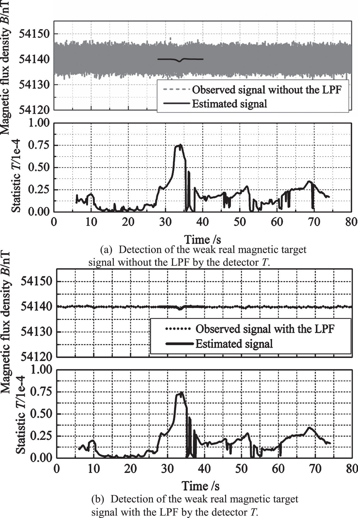
Detection of the weak real magnetic target signals by the detector T.

Table 6

Estimated parameters by the NPD-EM algorithm from the weak real magnetic target signals in the experiment

Signal	${\hat{a}}_{1} / 10^{- 2}$	${\hat{a}}_{2} / 10^{- 2}$	${\hat{a}}_{3} / 10^{- 2}$	${\hat{R}}_{0} / - M$	t₀/s
Without LPF	– 0.28	0.50	– 0.66	1.185	34
With LPF	– 0.26	0.45	– 0.69	1.188	33.7

From Fig. 15, it can be seen that the statistic appears an evident peak around the 34th second, no matter the LPF is employed or not. The time the statistic peaks accords with the recorded time the detector reaches the CPA point. Thus, the detector T based on the NPD-EM algorithm is feasible.

Comparing Fig. 15(a) and 15(b), the detection results with and without the LPF are extremely similar. It is because of the statistic T. In the detector, the statistic T is corresponding to the unbiased estimator of the efficient signal energy, and the innovative compensation $- 3 \hat{J}$ from the NPD-EM algorithm would reduce the impact from the noise, no matter the LPF is employed or not. In other words, the statistic T with the innovative compensation can automatically remove some noise influence as a filter and can guarantee the performance.

Besides, the LPF still has some adverse impacts on the detection and estimation performance, though the LPF can enhance the SNR from –17 dB to 4.2 dB. First, compared with the statistic’s peak without the LPF, the statistic’s peak with the LPF is reduced 1.6%. Second, without the LPF, the time the statistic peaks hits the recorded time the detector reaches the CPA point. While, with the LPF, the error between the time the statistic peaks and the recorded time the detector reaches the CPA point are 0.3 seconds. Third, the estimation of the latent variable without the LPF is more accurate than the one with the LPF. The reason of these adverse impacts is that the target signal preprocessed by the LPF would be distorted and would lose its characteristics in high frequency bands. So, the LPF is not recommended in the application of the NPD-EM algorithm and the corresponding detector.

6 Conclusion

This paper proposes a novel NPD-EM algorithm for the estimation and detection of a magnetic dipole signal with a latent variable at low SNRs. From related studies, the following conclusions can be drawn:

The latent variable, which is in the orthogonal model of the weak magnetic dipole signal, impacts the amplitude and effective width of the unit orthogonal basis functions. The unit orthogonal basis functions constructed with an inaccurate latent variable would lose their unit orthogonality with the real signal model and impact the estimation and detection.

The NPD-EM algorithm can accurately and efficiently estimate the magnetic dipole signal with a latent variable at low SNRs. It overcomes an unknown probability distribution which disables the standard EM algorithm and makes the traditional EM algorithm need huge calculated amount. In the NPD-EM algorithm, the estimation error of the parameters and latent variable are less than 0.3% of the corresponding true values in noise-free signals, which is comparable with the traditional EM algorithm. And the calculated amount of the NPD-EM algorithm is 3 orders of magnitude less than the calculated amount of the traditional EM algorithm. In additive white Gaussian noise, when the SNR is over –34 dB, the deviations between the true values and the expectations of the estimated parameters are less than 4% of the corresponding true values, and the maximum variance of the estimated parameters is 9.79% of the corresponding true values.

The detector T based on the NPD-EM algorithm has outstanding detection performance of the weak magnetic dipole signal, in which the statistic represents the unbiased estimator of the magnetic dipole signal energy and the introduced innovative compensation reduces the noise influence. In additive white Gaussian noise, when the SNR is over –34 dB, the detector T is comparable to the ideal matching filter which is the optimal detector in time-domain; when the SNR is –36 dB and the false alarm probability is 0.01, the detection probability can be 0.99; when the SNR is –38 dB and the false alarm probability is 0.05, the detection probability can be 0.96. Besides, the detector T would no longer be impacted by the latent variable when the SNR is over –34 dB, due to the excellent performance of the NPD-EM algorithm.

The NPD-EM algorithm and the corresponding detector can also be applied to estimate and detect real magnetic target signals in real colored noise. In the experiments with real magnetic targets and colored noise, the estimation error of the NPD-EM algorithm on a magnetic target signal is 4.59%, and the detector based on the NPD-EM algorithm is effective when the SNR is –17 dB. Besides, a low pass filter is not recommended, due to its adverse impacts and the superiority of the constructed detector.

Footnotes

Acknowledgments

This research is supported by the National Key R&D Program of China (Grant Number 2017 YFF0107400).

References

Iacca

, Bakker

F.L.

, Wörtche

, Real-time magnetic dipole detection with single particle optimization, Applied Soft Computing 23 (2014), 460–473.

Zhu

, Liao

, Yang

, Tao

, A New Method for Radar High-Speed Maneuvering Weak Target Detection and Imaging, IEEE Geoscience & Remote Sensing Letters 11(7) (2014), 1175–1179.

Pan

, Liu

D.J.

, Guo

Z.Y.

, Fang

H.F.

, Feng

M.Q.

, Magnetic anomaly inversion using magnetic dipole reconstruction based on the pipeline section segmentation method, Journal of Geophysics & Engineering 13(3) (2016), 242–258.

Ege

, Nazlibilek

, Kakilli

, Çıtak

, Kalender

, Erturk

K. L.

, Sengul

and Karacor

, A Magnetic Measurement System and Identification Method for Buried Magnetic Materials Within Wet and Dry Soils, IEEE Trans Geosci Electron 54(3) (2016), 1803–1811.

Zhang

, Wang

, Guo

, Research of extremely low frequency to magnetic dipole in seawater media, Int Conf on Information and Communications Technologies IET (Xi’an, China) (2015), 1–6.

Holmes

, Reduction of a Ship’s Magnetic Field Signatures, Morgan & Claypool 2 (2008), 1–68.

Ginzburg

, Frumkis

, Kaplan

B.Z.

, Processing of magnetic scalar gradiometer signals using orthonormalized functions Sens, Actuators A 102(1-2) (2002), 67–75.

Ginzburg

, Frumkis

, Kaplan

B.Z.

, Sheinker

, Salomonski

, Investigation of advanced data processing technique in magnetic anomaly detection systems, Int J Smart Sens Intell Syst 1(1) (2008), 110–122.

Zhou

, Xiao

, Liu

, Magnetic moments estimation and localization of a magnetic object based on Hopfield neural network, Automation Congress IEEE (Hawaii, HI, USA) (2008), 1–5.

10.

Umurkan

, Koroglu

, Kilic

, Adam

A.A.

, A neural network based estimation method for magnetic shielding at extremely low frequencies, Expert Systems with Applications 37(4) (2010), 3195–3201.

11.

, Wang

, Sun

, Target positioning and parameter estimation of magnetic dipole model with nonlinear least square method, Int Cong on Image and Signal Processing IEEE (Dalian, China) (2015), 923–927.

12.

Guo

, Tan

, Cai

, Estimation and detection of the weak transient ELF signal based on the phase inverting double-peak exponential model, Yi Qi Yi Biao Xue Bao/chinese Journal of Scientific Instrument 8 (2015), 1682–1691.

13.

Dempster

A.P.

, Maximum likelihood estimation from incomplete data via the EM algorithm, Journal of the Royal Statistical Society (1977), 1–38.

14.

Birsan

, Measurement of the extremely low frequency (ELF) magnetic field emission from a ship, Meas Sci Technol 22(8) (2011), 085709.