Prediction of a multi-mode coupling model based on traffic flow tensor data

Abstract

The modeling and prediction of short-term traffic flow can reflect the prediction results of the traffic state and traffic flow data. In this paper, first, we use a high-dimensional tensor to represent the multi-mode characteristics of traffic flow data, and we make use of the basic operations properties of tensors, such as Tucker decomposition, to study the methods for filling in data, such as ITRM. Additionally, we preprocess the lost traffic flow and abnormal data. At the same time, we study the short-term traffic flow based on the “week-day-time” multi-mode of the traffic flow data. Using the grey model (GM (1, 1)) to predict the same period of the weekly mode, the scrolling grey model (SGM) of the same time period is predicted. For the time mode, a neural network time series of wavelet analysis is used to predict the traffic flow forecast during the same period. Then, the prediction results of the three different models are weighted by the grey correlation analysis method, and then, the coupling prediction model of the three models is obtained. In the end, according to the traffic flow data of the main road of Shaoshan road in Changsha, Hunan, China, we first preprocess the lost data by using the filling algorithm for the tensor data, and then, we make the traffic flow data complete, use the three tensor data modes of traffic flow, and analyze the results. The experimental results show that the coupling prediction model with the tensor model is much better than the single GM (1, 1) model, the SGM and the neural network prediction model.

Keywords

High-dimensional tensor multi-mode traffic flow data short-term traffic flow forecasting grey model

1 Introduction

The traffic control system, traffic management system and traffic guidance system are important parts of an Intelligent Transportation System (ITS). Traffic prediction based on real-time traffic information is the premise of real-time control and induction, and it is an important theoretical basis of an ITS. The effective method of studying short-term traffic flow modeling and prediction theory can reflect the prediction results of the traffic flow data. It is directly applied to the advanced traffic information system (ATIS) and the advanced traffic management system (ATMS), and it provides travelers with real-time and effective travel information, such as stroke data, expected delay and path information. This information helps travelers to better choose paths, to realize path induction, to save time, to alleviate short circuit congestion, to reduce pollution, to save energy and so on. Traffic flow data from time and space contains rich multi-mode features [1]. It is still a difficult problem to make full use of the multi-mode characteristics of the traffic data in a unified framework. A tensor is a multidimensional array. It is a generalization of vector and matrix models to multidimensional data. It can represent the characteristics of multi-modal traffic data. According to the different modes of traffic flow data over a week, day, time and space, a multidimensional tensor can be used to overcome the issue that vector data flow and matrix data flow are difficult to characterize in terms of multidimensional features [2]. The traffic flow tensor mode [3] is constructed, and the short-term traffic flow prediction theory and method under the tensor multi-mode framework can be studied, which means that the traffic data can be better excavated in over a week, day, time and space. The characteristic of having multiple modes serves to the benefit of short-term traffic flow prediction.

Most of the functions of the subsystems of intelligent transportation systems are based on the complete and available traffic data. However, due to the breakdown of the detection equipment, transmission equipment and so on, the original traffic data often have the phenomena of data loss and data anomalies, which brings adverse effects to the analysis of traffic data and the deep mining of the actual traffic information system. In addition, the lost and abnormal traffic data have substantial impacts on the traffic information system and other intelligent transportation systems based on this system [4]. Traffic prediction, which is the key technical basis of intelligent transportation systems, requires complete historical data to obtain more accurate predictions. In the case of loss of traffic data, a traffic prediction model becomes especially sensitive, which leads to large error prediction. Therefore, according to the data characteristics of the tensor multi-mode, the traffic data are restored [5 –8]. The clean, accurate, and structured traffic data information is the basis of the efficient operation of the intelligent transportation system.

Autoregressive Integrated Moving Average Model [9] is widely used in short-term traffic flow prediction and is based on vector data flow. The local chaos prediction model [10], support vector machine (SVM) [11] and others have better prediction effects on the link travel traffic flow. The short-term traffic flow prediction in the form of matrix data flow mainly includes a multivariable time series prediction model [12] and multi-section short-term traffic flow prediction, which are applications from Yibing Wang et al. [13] that have been popularized by the Kalman filter method to predict the real time traffic flow on an expressway. At the same time, researchers have studied the significant periodicities in traffic flow data, especially in the week-mode and day-mode [14], which improve the accuracy of short-term traffic flow prediction. Guo et al. [15] considered seasonal characteristics in the traffic flow data to predict the traffic flow in real time. Zhang and others [16] analyzed traffic data cycle trends, certainty and volatility to study traffic flow prediction, and all of these approaches had good results.

At the same time, the grey model is adaptable, and it can handle mutation parameters. Since the founding of [17] in 1982, the grey prediction model has been a core part of grey system theory. It has been widely applied in various fields [18 –21]. Among them, short-term traffic flow prediction is an important application aspect. Xiao et al. [22] proposed a seasonal grey GM (1,1) rolling prediction model based on a periodic truncation accumulating operator (CTAGO). Guo et al. [23] established a grey nonlinear delayed GM (L, l) model to pretest the short time traffic flow of urban roads. Bezuglov and Comert [24] improved the Fourier error by improving the GM (L, l) model and grey Verhulst model, and they applied them to traffic flow prediction. On the other hand, wavelet analysis has good time frequency loal-ization. It is applied in the field of traffic flow prediction with a combination of wavelet theory and other algorithms, and a combination of wavelet theory and neural networks [25 –27] can obtain better results.

However, in view of the above short-term traffic flow forecasting methods, it is found that most of the prediction methods are based on a single prediction model, while a single prediction model cannot guarantee absolute good performance indicators, and the combined model can obtain different information from different perspectives and different models. After learning from each other, the model can improve the accuracy and stability of the model prediction. The MA model is used to forecast the trends of the week by Tan et al. [28], forecasting the intraday trends by using an ARIMA model, while a neural network is used for data aggregation. Chan et al. [29] introduced the hybrid exponential smoothing method and the least square method into a neural network model. Their experiment proves the effectiveness and feasibility of the combined prediction model for traffic flow prediction. Wang et al. [30] integrated the Bayes ensemble method, ARIMA model, Kalman filter and three other models. In addition, the researchers used ARIMA [31, 32] combined with other models for short-term traffic flow prediction to achieve better results.

However, the above combined predictive models concern only time information and only pay attention to the characteristics of nonlinearity, volatility and periodicity in the single time series change of the target section, and they fail to make full use of the time information features of traffic flow data; thus, the prediction results are affected in this way. Therefore, to better excavate the characteristics of traffic data in the three modes of week, day and time, this paper uses a high-dimensional tensor model to represent the multi-mode data characteristics of the traffic flow data. First, we study the lost and abnormal aspects of the traffic flow data, and we use the basic operational properties of tensor Tucker decomposition to study the method of tensor filling data using ITRM and other approaches. The traffic flow loss and abnormal data are pretreated effectively to obtain clean, accurate and structured traffic data. We discuss the tensor “week - day - time” mode, and for the same time cycle mode, the classical GM (1,1) model is used for the prediction. For the day mode, we use the SGM. We forecast the traffic flow data at the same time over two weeks; we obtained the forecasting data, removed the old information and added new information to predict the next data, and then, we repeated the previous process and completed the prediction of the subsequent part of the data. For the time mode, a prediction method with good time frequency localization properties and neural networks is applied. Then, the prediction data over the same time period obtained by the three models are correlated with the original data by the grey correlation analysis method, and the different correlation coefficients are obtained. According to the correlation coefficients, the different weights of the three models are obtained, and the final prediction results are obtained according to the different weights. Finally, we take the 7:00–9:00 traffic flow data of the main road of the Shaoshan road in Changsha, Hunan as an example. According to the multi-mode characteristics of the data, three typical tensor models of “week - day - time” are established. First, we use the filling algorithm of the tensors for the missing data, and we make an empirical analysis of the data filling technology. Then, for the traffic flow prediction at the same time, three different tensor models are compared, and the experimental results show that the simulation and prediction effects of the coupling of the three models for the tensor is better than the GM(1,1) model, SGM model and wavelet analysis of neural network.

The sections in this paper are arranged as follows: The second section introduces the multi-modal characteristics of the traffic flow data tensor and introduces the filling algorithm that includes a tensor based on the operational properties of the tensors. In the third section, we use different tensor models to express the characteristics of the multimodal data of the traffic flow, and we introduce three different models and grey relational analysis. In the fourth section, we preprocess the traffic flow data and analyze the results of the coupling model and individual method. The last section is the conclusions.

2 High-dimensional tensor pattern data filling method

2.1 Decomposition model of tensors

A tensor is a multi-dimensional array that is composed of data. It can be seen as a further extension of vectors and matrices in high-dimensional space. It is composed of multi-dimensional arrays or multi-dimensional matrices. For example, a vector can be regarded as a 1-order tensor, and a matrix can be regarded as a 2-order tensor. Here are some related concepts [33]:

Definition 2.1. N-order tensor χ ∈ R^{I₁×I₂×⋯×I_N} can be expanded to a matrix at any order, reordering the tensor elements into $I_{n} \times \prod_{j = 1, j \neq n}^{N} I_{j}$ dimensional matrix X⁽ⁿ⁾, the (i_n, k) element is x_{i₁i₂⋯i_N}, and among them, $k = 1 + \sum_{m = 1, m \neq n}^{N} ((i_{m} - 1) \prod_{m^{'} = 1, m^{'} \neq n}^{m} I_{m^{'}} .$

This process is called tensor n-mode matrixing.

Definition 2.2. Set two N-order tensors χ ∈ R^{I₁×I₂×⋯×I_N} and y ∈ R^{I₁×I₂×⋯×I_N}; then, $< χ, y > = \sum_{i_{1} = 1}^{I_{1}} \sum_{i_{2} = 2}^{I_{2}} \dots \sum_{i_{N} = 1}^{I_{N}} x_{i_{1} i_{2} \dots i_{N}} y_{i_{1} i_{2} \dots i_{N}}$

is called the inner product of two N-order tensors.

Definition 2.3. Set N order tensors χ ∈ R^{I₁×I₂×⋯×I_N}, and define the Frobenius norm as follows: $∥ χ ∥ = \sqrt{〈 χ, χ 〉} = \sqrt{\sum_{i_{1} = 1}^{I_{1}} \sum_{i_{2} = 1}^{I_{2}} \dots \sum_{i_{n} = 1}^{I_{n}} x_{i_{1} i_{2} \dots i_{N}}^{2}} .$

The Frobenius norm is also called the tensor modulus.

Definition 2.4. Set N-order tensors χ₁ ∈ R^{I₁×I₂×⋯×I_N} and M-order tensors χ₂ = R^{I₁×I₂×⋯×I_M}, then $χ_{1} \otimes χ_{2} = x_{i_{1} i_{2} \dots i_{N}} y_{i_{1} i_{2} \dots i_{M}},$

which is called the outer product of two tensors.

Definition 2.5. If N-order tensors χ ∈ R^{I₁×I₂×⋯×I_N} can be expressed as a form of N vector exterior product: χ = x₁ ⊗ x₂ ⊗ ⋯ ⊗ x_N, x_k ∈ R^I_k (k = 1, 2, …, N), then the tensor χ is a rank-1 tensor.

2.2 Iterative tensor Tucker decomposition data recovery method

Tucker decomposition is proposed by Tucker in 1963 about Principal Component Analysis of higher order. It expresses a tensor as a core-tensor multiply by a matrix along each mode. Afterward, tucker decomposition is mainly used to matrix singular threshold decomposition in high dimensional space which called Higher Order Singular Value Decomposition (HOSVD). To learn more about tucker decomposition, we introduce two common decomposition model, CP decomposition and Tucker decomposition [32].

The CP decomposition model is used to decompose the N-order tensor χ ∈ R^{I₁×I₂×⋯×I_N} into a number of rank-1 tensor sums: $\begin{matrix} χ & \approx & [A^{(1)}, A^{(2)}, \dots, A^{(N)}] \\ = \sum_{r = 1}^{R} a_{r}^{(1)} \otimes a_{r}^{(2)} \otimes \dots \otimes a_{r}^{(N)} . \end{matrix}$

The factor matrix of tensor χ as follow: $\begin{matrix} A^{(1)} = (a_{1}^{(1)}, a_{2}^{(1)}, \dots, a_{R}^{(1)}), A^{(2)} = (a_{1}^{(2)}, a_{2}^{(2)}, \dots, a_{R}^{(2)}) \\ , \dots, A^{(N)} = (a_{1}^{(N)}, a_{2}^{(N)}, \dots, a_{R}^{(N)}) \end{matrix}$

R is an integer.

For three order tensor χ ∈ R^I×J×K, its CP decomposition as follow: $\begin{matrix} χ \approx [λ, A, B, C] = \sum_{r = 1}^{R} λ_{r} a_{r} \otimes b_{r} \otimes c_{r}, \\ a_{r} \in R^{I}, b_{r} \in R^{J}, c_{r} \in R^{K}, r = 1, 2, \dots, R . \end{matrix}$

The corresponding element of tensor χ: $\begin{matrix} x_{ijk} & \approx & \sum_{r = 1}^{R} a_{ir} \otimes b_{jr} \otimes c_{kr}, i = 1, 2, \dots, I; \\ j = 1, 2, \dots, J; k = 1, 2, \dots, K . \end{matrix}$

Figure 1 shows a schematic diagram of a third-order tensor decomposition.

Fig. 1.

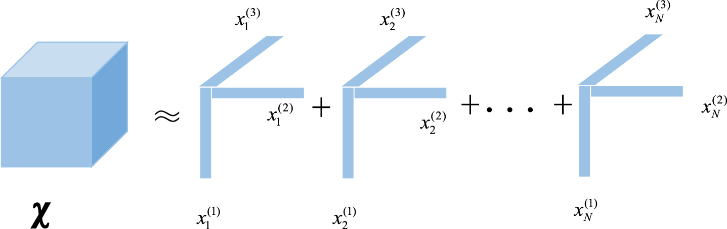
CP decomposition of third-order tensors.

Tucker decomposition of tensors aims to decompose the N-order tensor χ ∈ R^{I₁×I₂×⋯×I_N} into low-dimensional kernel tensors χ₃ ∈ R^{R₁×R₂×⋯×R_N} and the N factor matrix product model

$\begin{matrix} A^{(n)} \in R^{I_{n} \times R_{n}}, n = 1, 2, \dots, N : \\ χ \approx [χ_{3} : A^{(1)}, A^{(2)}, \dots, A^{(N)}] \\ = χ_{3} \times_{1} A^{(1)} \times_{2} A^{(2)} \times \dots \times_{N} A^{(N)} . \end{matrix}$

The factor matrix A⁽¹⁾, A⁽²⁾, ⋯ , A^(N) always orthonormal. The element of tucker decomposition as follow: $x_{i_{1} i_{2} \dots i_{N}} \approx \sum_{k_{1} = 1}^{R_{1}} \sum_{k_{2} = 1}^{R_{2}} \dots \sum_{k_{N} = 1}^{R_{N}} r_{k_{1} k_{2} \dots k_{N}} a_{i_{1} k_{1}}^{(1)} a_{i_{2} k_{2}}^{(2)} \dots a_{i_{N} k_{N}}^{(N)} .$

The matrix form of tucker decomposition as follow: $X_{(n)} \approx A^{(n)} R_{(n)} {(A^{(N)} \otimes \dots \otimes A^{(n + 1)} \otimes A^{(n - 1)} \otimes \dots \otimes A^{(1)})}^{T} .$

For instance, for three order tensor χ ∈ R^{I₁×I₂×I₃}, if $R \times_{1} A \times_{2} B \times_{3} C$ matriculated each side simultaneous, then the tucker decomposition of three order tensor can be expressed as: $\begin{matrix} X_{(1)} \approx {AR}_{(1)} {(C \otimes B)}^{T}, X_{(2)} \approx {BR}_{(1)} {(C \otimes A)}^{T}, \\ X_{(3)} \approx {AR}_{(3)} {(B \otimes A)}^{T} . \end{matrix}$

Figure 2 shows the Tucker decomposition of the third-order tensor.

Fig. 2

Tucker decomposition of a third-order tensor.

CP decomposition can be considered as a special form of tucker decomposition. If core tensor $R$ is diagonal and r₁ = r₂ = ⋯ = r_n, then tucker decomposition retrograde to CP decomposition.

According to the principle of tucker decomposition, we introduce the process of recovery by tucker decomposition:

The tensor χ and the sheltered tensor Omega which means that some data of tensor are missing are superimposed to obtain a tensor with missing data B = χ_· * O_mega. In the process of an iteration, we first decompose the original tensor B′ = B to obtain the kernel tensor L and a series of singular value matrices U¹⁽¹⁾, U¹⁽²⁾, ⋯ , U^1(N), where 1 in front of the bracketed bracket indicates the number of iterations; then, there are $B^{'} = L \times_{1} U^{1 (1)} \times_{2} U^{1 (2)} \dots \times_{N} U^{1 (N)} .$

From the Tucker decomposition principle and process introduced above, it can be known that the tensor n-th order singular matrix is the left singular matrix that corresponds to the tensor n-th order matrix, and thus, the N singular value matrix of Tucker decomposition of N-order tensors is calculated. The process can be seen as calculating N times the size of I_n = I₁I₂ ⋯ I_n-1I_n+1 ⋯ I_N (1 ≤ n ≤ N).

With Tucker decomposition of the different matrices of the matrix in such a way that a singular matrix can be found U¹⁽¹⁾, U¹⁽²⁾, ⋯ , U^1(N), nuclear tensors can pass B′, and we have a series of singular matrix calculations: $L = B^{'} \times_{1} U^{1 (1) T} \times_{2} U^{1 (2) T} \dots \times_{N} U^{1 (N) T} .$

Then, select k₁, k₂, ⋯ , k_N singular vectors in the front of each singular value matrix, and the number of singular vectors can be chosen based on experience. Then, we obtain a matrix B¹ similar to B′. Additionally, let $\begin{matrix} {\tilde{U}}^{1 (1)} = U^{1 (1)} (:, 1 : k_{1}), {\tilde{U}}^{1 (2)} = U^{1 (2)} (:, 1 : k_{2}), \\ \dots, {\tilde{U}}^{1 (N)} = U^{1 (N)} (:, 1 : k_{N}) . \end{matrix}$

At this time, we have the nuclear tensor

$\tilde{L} = L (1 : k_{1}, 1 : k_{2}, \dots, 1 : k_{N})$ . Therefore, $B^{1} = \tilde{L} \times_{1} U^{1 (1) T} \times_{2} U^{1 (2) T} \dots \times_{N} U^{1 (N) T}$

We extract the missing part of the tensor and restore it to the original missing data tensor B. The missing data part of the tensor ${\tilde{B}}^{1}$ has the following results: ${\tilde{B}}^{1} = B + B^{1} * (1 - O_{mega})$

Next, using Tucker decomposition for the new tensor ${\tilde{B}}^{1}$ , we can obtain the similar tensor B¹. While it is possible to restore the missing data of B² to the original matrix B to obtain the measured ${\tilde{B}}^{2}$ , repeat the entire process until the objective function converges. It can be seen that at each iteration, the similarity matrix is closer to the true tensor, and the missing elements are also closer to the true value. It can be seen that the objective function of the above process is convergent, and ultimately, the missing data can be recovered by using the feature contribution of the principal component and the internal relationship between the tensor elements in the Tucker decomposition process.

When the iteration process satisfies the convergence condition, the missing data recovery process completes the evaluation of the data recovery. The following error calculation formula was used: $Error = \frac{\sum | (B - \tilde{B}) * (1 - O_{mega}) |}{Nmis}$

The numerator represents the sum of the absolute value error in the sheltered part, and Nmis represents the number of sheltered elements in the tensor. Because the main basis for the algorithm is the known elements in the tensor and the value of the known elements do not change, the part that must be evaluated is only the missing data part.

The above are the process of tucker-decomposition, it aims to figure out a new tensor $R$ by means of iterative decomposition on tensor χ which lost some data. The ITRM algorithm [33] is used to implement the tensor Tucker threshold method in an iterative form for the reconstruction process with missing data tensors. The algorithm uses tensor principal components to recover the missing data. The following is the iterative tensor Tucker decomposition method for data recovery: the ITRM algorithm. The algorithm is given in Table 1.

Table 1

ITRM algorithm

ITRM algorithm: Iterative tensor Tucker decomposition data recovery method
Input: χ ∈ R^{I₁×I₂×⋯×I_N}, the rank of χ is k₁, k₂, ⋯ , k_N, Omega, Iter_max .
Set B′ = B, calculate the Tucker decomposition of B′
1.	Repeat
2.	for n ← 1 to N
3.	B (n) ← U⁽ⁿ⁾Σ⁽ⁿ⁾V⁽ⁿ⁾
4.	end
5.	L ← B′ × ₁U^(1)T × ₂U^(2)T ⋯ × _NU^(N)T
6.	${\tilde{B}}^{'} \leftarrow L (1 : k_{1}, 1 : k_{2}, \dots, 1 : k_{N}) \times_{1} U^{(1)} (:, 1 : k_{1}) \dots \times_{N} U^{(N)} (:, 1 : k_{N})$
7.	B¹ ← B + B′ * (1 - O_mega)
8.	$B^{'} \leftarrow {\tilde{B}}^{1}, i \leftarrow i + 1$
9.	Computer Error
10.	Until i ≤ Iter_max
11.	Output: χ

ITRM algorithm realize the tensor reconstruction by tensor Tucker threshold iterative method. In the algorithm, the data are in the form of tensor. Through tucker decomposition we get the potential structure of those items of tensor, then extract the principal component of tensor to realize the reconstruction of missing data.

2.3 Experiments on the data recovery method of the iterative tensor Tucker decomposition

The data used in this study are obtained from the Urban Transportation Research Institute of Central South University [34]. The selected data were derived from four straight lines in the direct direction of Shaoshan Road from south to north in Changsha, China. The collector collects the traffic flow every five minutes, and there are a total of 63 days of traffic flow from September 17, 2013 to November 18, 2013.

To verify the convergence of the algorithm, we make a comparative analysis from three aspects. First, a tensor χ was randomly generated on Wednesday and Saturday’s five-minute data, according to the continuous 63-day week. The missing data make up 50% (these data we don’t know). The mean absolute percentage error (MAPE) and iterative times are used in the algorithm’s convergence process, as shown in Fig. 3.

Fig. 3

The convergence graph of the 50% loss rate.

Figure 3 shows that the algorithm can converge after approximately 10 iterations. It shows that the convergence speed of ITRM is better at filling in the initial incomplete traffic flow data, and the following experiments were conducted according to the traffic flow data. For different loss rates, when the loss rate increased from 0.1 to 0.9 with a step length of 0.1, the experiment was compared and analyzed. The following is a comparison of the data from the data of Friday in 63 days.

Figure 4 shows that when the loss rate is between 0.1 and 0.6, there is almost a smooth linear increase between the MAPE and the loss rate. Additionally, the error is relatively small for the five-minute interval traffic flow data, within acceptable limits. The figure shows that the ITRM algorithm in this range can achieve better experimental results in implementing the data recovery. Because the algorithm can successfully restore the unknown data in the traffic flow tensor, the equipment that currently tests the transportation equipment is also advanced, and the data that are lost in the experimental section of 63 days are less than 10%. Therefore, we choose this method to preprocess the data. Figure 5 represents the 16th day of the nine weeks (October 2nd). The experimental comparison diagram of the lost data and recovered data is shown below:

Fig. 4

Comparison of the loss rate from 0.1 to 0.9.

Fig. 5

Data-filled diagram for 20-minute intervals on October 2nd.

3 Model introduction

This section mainly introduces the GM(1,1) prediction model, GM (1,1), the SGM prediction model, and the model based on the wavelet network, in addition to the grey relational analysis.

3.1 GM (1,1)model

Set the original sequence to be $X^{(0)} = (x^{(0)} (1), x^{(0)} (2), \dots, x^{(0)} (n)),$ (3.1)

An accumulative generation sequence of the original sequence is $X^{(1)} = (x^{(1)} (1), x^{(1)} (2), \dots, x^{(1)} (n))^{T}$ (3.2) where $\begin{matrix} x^{(1)} (k) & = & AGO (x^{(0)} (i)) \\ = & \sum_{i = 1}^{k} x^{(0)} (i), k = 1, 2, \dots, n \end{matrix}$

In addition, set Z⁽¹⁾ = (z⁽¹⁾ (2) , x⁽¹⁾ (3) , ⋯ , z⁽¹⁾ (n)) ^T as the adjacent mean equal weight-generating sequence of X⁽¹⁾ $z^{(1)} (k) = 0.5 x^{(1)} (k) + 0.5 x^{(1)} (k - 1) k = 2, 3, \dots, n .$ (3.3)

Definition 3.1. Set the sequences X⁽⁰⁾, X⁽¹⁾ and Z⁽¹⁾ according to (3.1–3.3), which is called the grey differential equation $x^{(0)} (k) + {az}^{(1)} (k) = b$

which is a grey system prediction model for first-order equations with a variable, referred to as the GM (1,1) model [17]. The equation $\frac{d x^{(1)}}{dt} + a x^{(1)} = b$

is called whitening equation of x⁽⁰⁾ (k) + az⁽¹⁾ (k) = b which called grey differential equation The parameter estimation of grey differential equation as follows: $\begin{matrix} (\begin{matrix} a \\ b \end{matrix}) = (B^{T} B)^{- 1} B^{T} Y \\ B = (\begin{matrix} - z^{(1)} (2) & 1 \\ - z^{(1)} (3) & 1 \\ ⋮ & ⋮ \\ - z^{(1)} (n) & 1 \end{matrix}), Y = (\begin{matrix} x^{(0)} (2) \\ x^{(0)} (3) \\ ⋮ \\ x^{(0)} (n) \end{matrix}), \end{matrix}$

The GM (1,1) grey model has the following conclusions

(1) The time response function (solution) of the whitening equation $\frac{d x^{(1)}}{dt} + a x^{(1)} = b$ is $x^{(1)} (t) = (x^{(1)} (1) - \frac{b}{a}) e^{- a t} + \frac{b}{a}$

(2) The time response sequence of the GM (1,1) grey differential equation: $\begin{matrix} {\hat{x}}^{(1)} (k + 1) & = & (x^{(0)} (1) - \frac{b}{a}) e^{- a k} + \frac{b}{a}, \\ k = 1, 2, \dots, n \end{matrix}$

(3) Then, the restored values of x⁽⁰⁾ is given by ${\hat{x}}^{(0)} (k + 1) = a^{(1)} ({\hat{x}}^{(1)} (k + 1)) = {\hat{x}}^{(1)} (k + 1) - {\hat{x}}^{(1)} (k), k = 1, 2, \dots, n .$

GM(1,1) model is classical model of grey forecast. It studies specially on poor data system which is uncertain and is well-adapted to handle better variational parameter, and it can be used in traffic tensor flow forecast at week-mode.

3.2 Rolling grey SGM(1,1) prediction model

Definition 3.2. Set sequence X⁽⁰⁾ as Equation (3.2), $\begin{matrix} Y^{(0)} = CTAGO (x^{(0)} (k)) = \sum_{j = 1}^{q} x^{(0)} (k + j - 1) \\ \forall k = 1, 2, \dots n - q + 1 . \end{matrix}$ (3.4)

which is called the cycle truncation accumulated generating operation (denoted CTAGO), where q is the number of elements in each cycle. Setting r = n - q + 1, the sequence $y^{(0)} = (y^{(0)} (1), y^{(0)} (2), \dots, y^{(0)} (r))$ (3.5)

becomes the cycle truncation accumulated generating operation (denoted as CTAGO).

Definition 3.3. Set Y⁽¹⁾ = (y⁽¹⁾ (1) , y⁽¹⁾ (2) , ⋯ , y⁽¹⁾ (r)) , and then,

$\begin{matrix} y^{(1)} (k) & = & \sum_{i = 1}^{k} y^{(0)} (i) = \sum_{i = 1}^{k} \sum_{j = 1}^{q} x^{(0)} (i + j - 1), \\ k = 1, 2, \dots, r \end{matrix}$ (3.6)

Here, y⁽¹⁾ (k) is called the 1-AGO sequence of the CTAGO sequence y⁽⁰⁾ (k).

In addition, we regard $Z_{2}^{(1)} = (z_{2}^{(1)} (2), z_{2}^{(1)} (3), \dots, z_{2}^{(1)} (n))^{T}$ as the adjacent mean equal weight generating sequence for X⁽¹⁾,

$\begin{matrix} z_{2}^{(1)} (k) & = & 0.5 y^{(1)} (k) + 0.5 y^{(1)} (k - 1) \\ k = 2, 3, \dots, n . \end{matrix}$ (3.7)

Definition 3.4. Set sequence Y⁽⁰⁾, Y⁽¹⁾, $Z_{2}^{(1)}$ to satisfy (3.4–3.6), and then, we call the grey differential equation

$y^{(0)} (k) + {az}_{2}^{(1)} (k) = b$

the grey system prediction model with a first-order equation with one variable, which is called SGM [21]. Its parameter estimation is as follows: $(\begin{matrix} a \\ b \end{matrix}) = (B^{T} B)^{- 1} B^{T} Y$

and $B = (\begin{matrix} - z_{2}^{(1)} (2) & 1 \\ - z_{2}^{(1)} (3) & 1 \\ ⋮ & ⋮ \\ - z_{2}^{(1)} (n) & 1 \end{matrix}), Y = (\begin{matrix} y^{(0)} (2) \\ y^{(0)} (3) \\ ⋮ \\ y^{(0)} (n) \end{matrix}) .$

SGM provides the following conclusions:

(1) The time response function (solution) of the whitening equation $\frac{d y^{(1)}}{dt} + a y^{(1)} = b$ is $y^{(1)} (t) = (y^{(1)} (1) - \frac{b}{a}) e^{- at} + \frac{b}{a}$ (3.8)

(2) The time response sequence of the $y^{(0)} (k) + {az}_{2}^{(1)} (k) = b$ of the GM(1,1) is as follows: ${\hat{y}}^{(1)} (k + 1) = (y^{(0)} (1) - \frac{b}{a}) e^{- ak} + \frac{b}{a}, k = 1, 2, \dots, n .$ (3.9)

(3) The recuperative values of x⁽⁰⁾ (k) as follow:

$\begin{matrix} {\hat{x}}^{(0)} (k + 1) & = & {\hat{y}}^{(0)} (k - q + 2) - y^{(0)} (k - q + 1) \\ + x^{(0)} (k - q + 1) \end{matrix}$ (3.10)

The grey rolling prediction SGM(1,1) prediction model is generalized form of classical grey model of GM(1,1). It applies the AGO of GM(1,1) to CTAGO of SGM(1,1). Each item of the y⁽⁰⁾ (k) is sum of cyclic data. Grey rolling SGM(1,1) uses former q item of data to forecast the (q+1) th data. Then, replace the oldest data of x⁽⁰⁾ (k + 1) with the predicted data, and so on.

This model can be used to forecast the traffic seasonal flow data. Through studying the cyclic raw, we can transform seasonal traffic flow data to mild sequence by means of limited past data and confirm the timeliness of forecast. Likewise, it can be used in day-mode forecast at the same time of each day.

3.3 Wavelet neural network

The wavelet neural network is a neural network that is based on the topology of the BP neural network, which takes the wavelet basis function as the transfer function of the hidden layer node, and the signal propagates forward while the error is propagated in reverse. When the input signal sequence is x_i = (i = 1, 2, ⋯ , k), the output formula of the hidden layer is $h (j) = h_{j} [\frac{\sum_{i = 1}^{k} ω_{i j} - b_{j}}{a_{j}}], j = 1, 2, \dots, l .$

Here, h (j) is the output value of the j nodes of the hidden layer; ω_ij is the connection weight of the input layer and the hidden layer; b_j is the shift factor of the small wave base function h_j; a_j is the expansion factor of the small wave basis function h_j; and h_j is a small wavelet basis function.

The wavelet basis function is the Morlet mother wavelet basis function, and the mathematical formula is $y = cos (1.75 x) e^{\frac{- x^{2}}{2}} .$

The output calculation formula of the wavelet neural network is $y (k) = \sum_{i = 1}^{1} ω_{ik} h (i), k = 1, 2, \dots, m .$

Here, ω_ik is the weight of the hidden layer to the output layer; h (i) is the output of the i-th hidden layer node; l is the number of hidden layer nodes; and m is the number of nodes in the output layer.

Wavelet neural network is better than neural network because its element and structure is decided by wavelet analysis theory, it avoids the blindness of BP neural network on structure design. It owns better learning skill and has faster, more accurate rate of convergence. Likewise, wavelet neural network has a better effect on short-time traffic flow forecast. It can forecast the whole trend of traffic flow. Consequently, it can be used to short-time traffic flow forecast of time-mode data.

3.4 Coupling of three models in tensor mode data

In traffic flow data, the traffic data between different weeks is correlated, and additionally, there is a stronger correlation between the weekday and weekend of a continuous week. Traffic flow data can be built into various forms of traffic flow data tensor models through a coupling mode. According to the characteristics of multiple modes of tensor data, a hybrid algorithm is used to predict the traffic flow data.

This paper collects traffic flow tensor data. Focusing on the correlation of traffic flow data, we adopted the “week-day-time” model. For the week model, we extracted data from the same time period in each week to build the sequence and adopted the classic GM(1,1) model for the prediction. The data of the day mode is seasonal, and the rolling seasonal SGM model based on the periodic truncation operator is used for the prediction. Focusing on the time-series data over time, we used the model of the neural network with wavelet analysis for the prediction. The predictive value of the data in the same time period on the same day of the week mode id was defined as $x_{t}^{m}$ , and its weight was defined as $w_{t}^{m}$ . The predicted value of the data during the same time period of the day mode is defined as $x_{t}^{n}$ , while its weight is defined as $W_{t}^{n}$ . Additionally, the predicted value of the data during the same time period of the time mode was defined as $x_{t}^{s}$ , and its weight is defined as $w_{t}^{s}$ . The coupling of three different prediction methods of the three modes is as follows: $x_{t} = w_{t}^{m} x_{t}^{m} + w_{t}^{n} x_{t}^{n} + w_{t}^{s} x_{t}^{s}$ (3.11)

The coupling algorithm is used to identify the weight of Deng’s grey relational degree [15]. The basic principle is to use the model fitting value and the actual value of the correlation degree. The higher the correlation degree of the model is, the higher the reliability, and the greater the weight in the coupling model. Conversely, the lower the correlation is, the lower the reliability, and the smaller the weight in the coupling model.

The definition of Deng’s grey correlation is as follows:

Definition 3.5. [15] Let X₀ = (x₀ (1) , x₀ (2) , ⋯, x₀ (n)), X_i = (x_i (1) , x_i (2) , ⋯ , x_i (n)).

These consequences have the same length. We define the grey relational degree of the vector as follows: $γ_{0 i} = \frac{1}{n} \sum_{k = 1}^{n} γ_{0 i} (k),$ $γ_{0 i} (k) = \frac{min_{i} min_{k} | x_{0} (k) - x_{i} (k) | + ξ max_{i} max_{k} | x_{0} (k) - x_{i} (k) |}{| x_{0} (k) - x_{i} (k) | + ξ max_{i} max_{k} | x_{0} (k) - x_{i} (k) |} .$ (3.12)

The coupling prediction model algorithm is as follows:

We extracted the fitting value and the real value sequence of the GM(1,1), SGM and Wavelet Analysis model.

According to formula (3.11), the corresponding close correlation degree $ρ_{t}^{m}, ρ_{t}^{n}, ρ_{t}^{s}$ is obtained.

The corresponding weighting coefficients in the coupling model are determined according to the degree of correlation:

$\begin{matrix} w_{t}^{m} = ρ_{t}^{m} / (ρ_{t}^{m} + ρ_{t}^{n} + ρ_{t}^{s}), \\ w_{t}^{n} = ρ_{t}^{n} / (ρ_{t}^{m} + ρ_{t}^{n} + ρ_{t}^{s}), \\ w_{t}^{s} = ρ_{t}^{s} / (ρ_{t}^{m} + ρ_{t}^{n} + ρ_{t}^{s}) . \end{matrix}$

4) According to formula (3.10), the time series and the cross-sectional data coupling predictive value are obtained:

The method of predicting the above is called a coupling model of tensor multi-mode data, and the prediction flow diagram is shown in Fig. 6

Fig. 6.

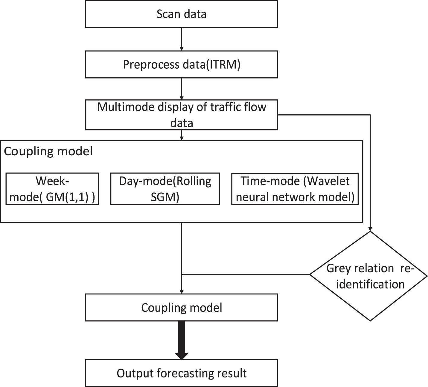
A flowchart of the data coupling model for the traffic flow in tensor mode.

4 Empirical analysis of the coupling model of the traffic flow tensor model

This section focuses mainly on the real-time data of traffic flows and fills in the lost data through the ITRM algorithm and through the properties of tensor operations. After filling in the traffic flow data, a tensor multi-mode representation is performed. For data of different tensor modes, the coupling model is empirically analyzed.

4.1 Establishment of traffic data model of tensor

Among traffic data, the traffic data of same day of different weeks have correlation, and especially the weekend of adjacent weeks. Hence, the correlation between several mode and traffic time-spatial data should be considered in traffic data model. We can express different forms of traffic data. Such as the tensor in location-week-day-time mode can be used to a traffic flow of some roads. We can get that: $χ \in R^{L \times W \times D \times T}, L = 11, W = 11, D = 7, T = 288$

Thereinto, L means loop, this model has 11 collectors, W means Weeks which contains 11 weeks data. D means Day which on behalf of that there are 7 days in a week. T means Time which shows that 288 times in a day.

Above model can be described as a week-day-time mode, and it also can be described as form like χ ∈ R^W×D×T; If set T = 288 = 24 × 12, denote the collect data each five minutes, 12 times an hour, then a five order tensor χ ∈ R^{11×11×7×24×12} can be derived. For time series, we can build different tensor model according different collected time. Such as collect data each ten minutes, than a five order tensor χ ∈ R^{11×11×7×24×6} can be derived.

After the traffic flow data are preprocessed, the data are collected by the collector every 5 minutes, and 288 data points can be collected in one day in section 2.3. Therefore, the third-order tensor form of the traffic data “week-day-time” can be obtained: χ ∈ R^9×7×288 tensor model, or fourth-order tensor, χ ∈ R^9×7×24×3, χ ∈ R^9×7×24×2, χ ∈ R^9×7×24×1, and so on. Here, 9 represents 9 weeks of data, 7 represents 7 days per week, 24 represents 24 hours per day, 2 represents two collection times per hour, 3 represents three collection times per hour, and 1 represents one collection per hour.

4.2 Analysis of the results of the tensor multi-mode data coupling model prediction

A comparative experiment for the first tensor model χ ∈ R^9×7×24×3 was compared to the experimental data with the data of 6 traffic flows every 20 minutes from 7:00 am to 9:00 am on Wednesday, November 14th. Here are the specific steps of the experiment:

Choose September 19, September 26, October 10, October 17, October 24, October 31, November 7, and November 14, removing the holiday on October 3. Data from 7:00–7:20 in the 8th week are forecasted using the GM (1,1) grey prediction model, and the 8th data point is predicted from the first 7 data points. The same method is used to predict the data for the other 5 periods.

For traffic flow from 7:00 to 7:20 on the 22nd day of November 14th, the real-time data from October 31 to November 14 are 14 days in length, and using the grey rolling prediction model SGM to predict the data for November 14th, the other time will also use the same method.

Using the 20-minute data from November 11 and November 13 for three days, a wavelet neural network model was used to predict the traffic flow data for 20 minutes between 7:00 and 9:00.

The data traffic predicted by the three models is correlated with the original data using formula (3.11), and then, the weights of the models are obtained by (3.10). The three models are coupled to obtain the final predicted values.

Compute and compare the predictive values and errors

Define the mean absolute percent error as follows: $MAPE = \frac{1}{n} \sum_{k = 1}^{n} \frac{| x^{(0)} (k) - {\hat{x}}^{(0)} (k) |}{x^{(0)} (k)} \times 100 %$ (4.1)

Here, x⁽⁰⁾ (k) represents the original data, and ${\hat{x}}^{(0)} (k)$ represents the predicted value.

The predictive values and errors of the coupling model, GM(1,1), SGM and wavelet analysis neural network models are depicted in Table 2.

Table 2

Simulation values and errors of the amount of the χ ∈ R^9×7×24×3 model

Serial number	Real data	GM(1,1)model	SGM model	Wavelet neural network model	Coupling model
1	344	365.31	371.22	348.95	362.08
2	491	505.10	490.56	484.03	493.36
3	569	591.96	603.94	530.11	575.97
4	515	525.96	487.14	436.70	483.99
5	474	490.91	472.15	460.82	474.82
6	492	493.88	486.85	489.21	489.97
MAPE		0.03180	0.03499	0.04708	0.02261

In Table 2, the effect of the coupling model depends on χ ∈ R^9×7×24×3 and is better than a single gray GM (1,1) model, gray rolling SGM model and wavelet neural network model. Among them, we have the GM (1,1) model predictive effect of the week-model and the day-mode gray rolling model SGM model, and the prediction results are comparable, while both are better than the wavelet neural network model. According to Table 1, the prediction percentage errors of the above three models for the traffic flow are illustrated in Fig. 7.

Fig. 7

Experimental comparison of coupling models and three single models.

As seen from Fig. 7, the effect of the coupling model depends on χ ∈ R^9×7×24×3 and is better than the three single models, which indicates that the coupling model is effective.

5 Conclusions

Traffic data provide an important data foundation for the research and development of intelligent transportation systems. The data contain rich multi-mode features. Tensors are a generalization of vector and matrix models, which can represent multidimensional data and exhibit multi-mode features. In this paper, multi-mode traffic flow data are represented by high-dimensional tensors, and a coupling model suitable for multi-mode state traffic flow is proposed. For comparison experiments, good results are achieved, specifically in the following areas:

To mine the characteristics of traffic data better in several modes such as week, day, and time, we attempt to fill in the lost traffic data and make use of Tucker decomposition and other basic computing properties; then, we preprocess the traffic flow data according to the ITRM algorithm to obtain whole and accurate traffic flow data.

We study the multi-mode characteristics of the traffic flow data and use different high-dimensional tensor models to represent different traffic flow data. According to the multi-mode correlation of traffic flow data, we use a classical gray GM (1,1) model for forecasting the week-mode data, use a grey rolling SGM prediction model to predict day-mode data and use a wavelet neural network for the time model prediction for the time-mode. Finally, three models are coupled according to the grey correlation technique.

Finally, we use the traffic flow data of 7:00–9:00 in the early peak period of the main road of Shaoshan Road in Changsha City, Hunan Province, China as an example for analyzing the data, and we establish the “week-day-time” mode according to the multi-mode characteristics of the data. Through comparative analysis, the experimental results show that the coupling model of the multi-mode data is better than the single model in terms of prediction effect.

Footnotes

Acknowledgments

This work is supported by the National Natural Science Foundation of China (No. 71871174, 71271226, 11671001). Project of Humanities and Social Sciences Planning Fund of Ministry of Education of China (18YJA630022).

References

Acar and

Yener , Unsupervised multiway data analysis: A literature survey, Knowledge and Data Engineering, IEEE Transactions on 21 (2009), 6–20.

M.A.O.

Vasilescu and

Terzoploulos , Multilinear(Tensor) image synthesis, analysis, and recognition, Signal Processing Magazine, IEEE 24 (2007), 118–123.

Tan and

Feng , et al., A tensor-based method for missing traffic data completion, Transportation Research Part C, Emerging Technologies 28 (2013), 15–27.

Chen and

S.S.

Grant-Muller , A study of hybrid neural network approaches and the effects of missing data on traffic forecasting, Neural Computing & Applications 3 (2001), 277–286.

Tan ,

Feng ,

Chen et al., Low multilinear rank approximation of tensors and application in missing traffic data, Advances in Mechanical Engineering (2014).

Tan ,

G.F.

Yang et al., Correlation analysis for tensor-based traffic data imputation method, Procedia-Social and Behavioral Sciences 96 (2013), 2611–2620.

Ran ,

Tan ,

Wu et al., Tensor based missing traffic data completion with spatial-temporal correlation, Physics A 446 (2016), 54–63.

Moniruzzaman ,

Maoh and

Anderson , Short-term prediction of border crossing time and traffic volume for commercial trucks: A case study for the Ambassador Bridge, Transportation Research part C-Emerging 63 (2016), 182–194.

Castro-Neto ,

Y.S.

Jeong et al., Online-SVR for short-term traffic flow prediction under typical and atypical traffic conditions, Expert Systems with Applications 36 (2009), 6164–6173.

10.

A.Y.

Cheng ,

Jiang and

Y.F.

Li , Muliple sources and multiple measures based traffic flow prediction using the chaos theory and support vector regression method, Physica A-Statistical Mechanics and ITS Applications 466 (2017), 422–434.

11.

Zhu ,

Peng and

C.F.

Xiong , Short-term traffic flow prediction with linear conditional Gaussian Bayesian network, Journal of Advanced Transportation 50 (2016), 1111–1123.

12.

Min and

Wynter , Real-time road traffic prediction with spatio-temporal correlations, Transportation Research Part C: Emerging Technologies 19 (2011), 606–616.

13.

Y.B.

Wang ,

Markos , Real-time freeway traffic state estimation based on extended Kalman filter: A general approach, Transportation Research Part B 39 (2005), 141–167.

14.

Chen ,

Wang ,

Li et al., The retrieval of intra-day trend and itsinfluence on traffic prediction, Transportation Research Part C: Emerging Technologies 22 (2012), 103–118.

15.

Guo ,

Huang and

B.M.

Williams , Adaptive Kalman filter approach for stochastic traffic flow rate prediction and uncertainty quantification, Transportation Research Part C: Emerging Technologies 43 (2014), 50–64.

16.

Zhang ,

Haghani , A hybrid short-term traffic flow forecasting method based on spectral analysis and statistical volatility model, Transportation Research Part C: Emerging Technologies 43 (2014), 65–78.

17.

J.L.

Deng , Estimate and decision of grey system, Wuhan: Huazhong University of Science and Technology Press, 2002.

18.

L.F.

Wu ,

S.F.

Liu and

Y.J.

Yang , et al., Multi-variable weakening buffer operator and its application, Information Sciences 339 (2016), 98–107.

19.

and Zhi

B.L.

, The GMC (1, n) model with optimized parameters and its application, The Journal of Grey System 29(4) (2017), 122–138.

20.

Zeng ,

H.M.

Duan and

Bai , Forecasting the output of shale gas in China using an unbiased grey model and weakening buffer operator, Energy 151 (2018), 238–249.

21.

L.F.

Wu ,

S.F.

Liiu ,

Y.J.

Yang , A gray model with a time varying weighted generating operator, IEEE Transactions on Systems Man Cybernetics-Systems 46 (2016), 427–433.

22.

X.P.

Xiao and Xiao , An improved seasonal rolling grey forecasting model using a cycle truncation accumulated generating operation for traffic flow, Applied mathematical Modelling 51 (2017), 386–404.

23.

Duan

H.M.

, Xiao

X.P.

and Pei

L.L.

, Forecasting the short-term traffic flow in the intelligent Transportation system based on an inertia nonhomogenous discrete grey model, Complexity (2017) 1–16.

24.

Bezuglov and

Comert , Short-term freeway traffic parameter prediction: Application of grey system theory models, Expert System Applied 62 (2016), 284–292.

25.

Yang ,

Hu , Wavelet neural network with improved genetic algorithm for traffic flow series prediction, International Journal for Light and Electron Optics 127 (2016), 8103–8110.

26.

Lin ,

Li and

Sadek , A k nearest neighbor based loacl linear wavelet neural network model for on-line short-term traffic volume prediction, Social and Behavioral Sciences 96 (2014), 2066–2077.

27.

Ma ,

Tao and

Wang , Long short-term memory neural network for traffic speed prediction using remote microwave sensor data, Transportation Research Part C: Emerging Technologies 54 (2015), 187–197.

28.

Tan ,

S.C.

Wong ,

Xu , et al., An aggregation approach to short-term traffic flow prediction, IEEE Transactions on Intelligent Transportation Systems 10 (2009), 60–69.

29.

K.Y.

Chan ,

T.S.

Dillon ,

Singh et al., Traffic flow forecasting neural networks based on exponential smoothing method, In: 2011 6th IEEE Conference on Industrial Electronics and Applications(ICIEA), Piscataway: IEEE, 2011, pp. 376–381.

30.

Wang ,

Deng and

Guo , New Bayesian combination method for short-term traffic flow forecasting, Transportation Research Part C: Emerging Technologies 43 (2014), 79–94.

31.

Wang ,

Liu ,

Qian , et al., Empirical mode decomposition-autoregressive integrated moving average, Transportation Research Record Journal of the Transportation Research Board 2460 (2014), 66–76.

32.

Wang ,

Papageorgiou and

Messmer , Real-time freeway traffic state estimation based on extended kalman filter: A case study, Transportation Science 41 (2007), 167–181.

33.

J.X.

Zhou ,

G.Y.

Qiu ,

S.G.

Liu , et al., Image restoration method with high order singular value decomposition of iterative tensor, Computer Application Research 6 (2013), 3488–3491.

34.

Li , Central South University Openits Data, .