
Abstract
A key component of many types of time series classification methods is an appropriate dissimilarity measure. Elastic measures like DTW, LCS, ERP and EDR are methods that have long been known in the time series community. The methods have flourished, particularly in the last decade, and have been applied to many real problems in a variety of branches. All of the above-mentioned measures have the common feature that they work in the time domain and equalize for possible localized misalignment through some elastic adaptation. However, being of quadratic time complexity, global constraints are often used to speed up computation. Apart from this advantage, it has been shown by simulations that constrained measures can also give better classification results than unconstrained measures.
In this paper, our aim is to verify experimentally the effects of the Sakoe–Chiba band on classification (by the 1NN method) with the above-mentioned measures. Using rigorous statistical analysis we demonstrate that it is possible to find global constraints which lead to improvement of the classification accuracy for all methods. Additionally, for each measure we suggest the best values of the parameter r (the size of the band).
Keywords
Introduction
A key element in dealing with time series is the use of an appropriate dissimilarity measure. There exist a large number of elastic dissimilarity measures used for time series analysis. The most popular are Dynamic Time Warping (DTW), Longest Common Subsequence (LCS), Edit Distance with Real Penalty (ERP), Edit Distance on Real Sequence (EDR) and Derivative Dynamic Time Warping (DDTW).
The implementation of each of these measures relies on dynamic programming. Such programming is quite slow and has some serious limitations when dealing with very large data. To improve the calculation time, various methods have been developed. It seems that because of its simplicity, the most popular is the Sakoe–Chiba band [30]. This constraint narrows the warping window around the diagonal using a single parameter R (Figure 1). The Sakoe–Chiba band is classified as global constraint. Another common such constraint is the Itakura parallelogram [19]. Global constraints are different from local constraints, because they do not provide local restrictions [21]. Ref. [23] reported that appropriately selected global constraints can significantly reduce the computation time of DTW and LCS. Additionally they noted that constrained variants of the above measures are qualitatively different from their unconstrained equivalents. Apart from reducing the computation time, the use of some constraints can lead to improved accuracy of classification with a nearest neighbors classifier, compared with unconstrained measures [2, 33]. Other recent papers devoted to the comparison of constrained dissimilarity measures are that of [10, 24].
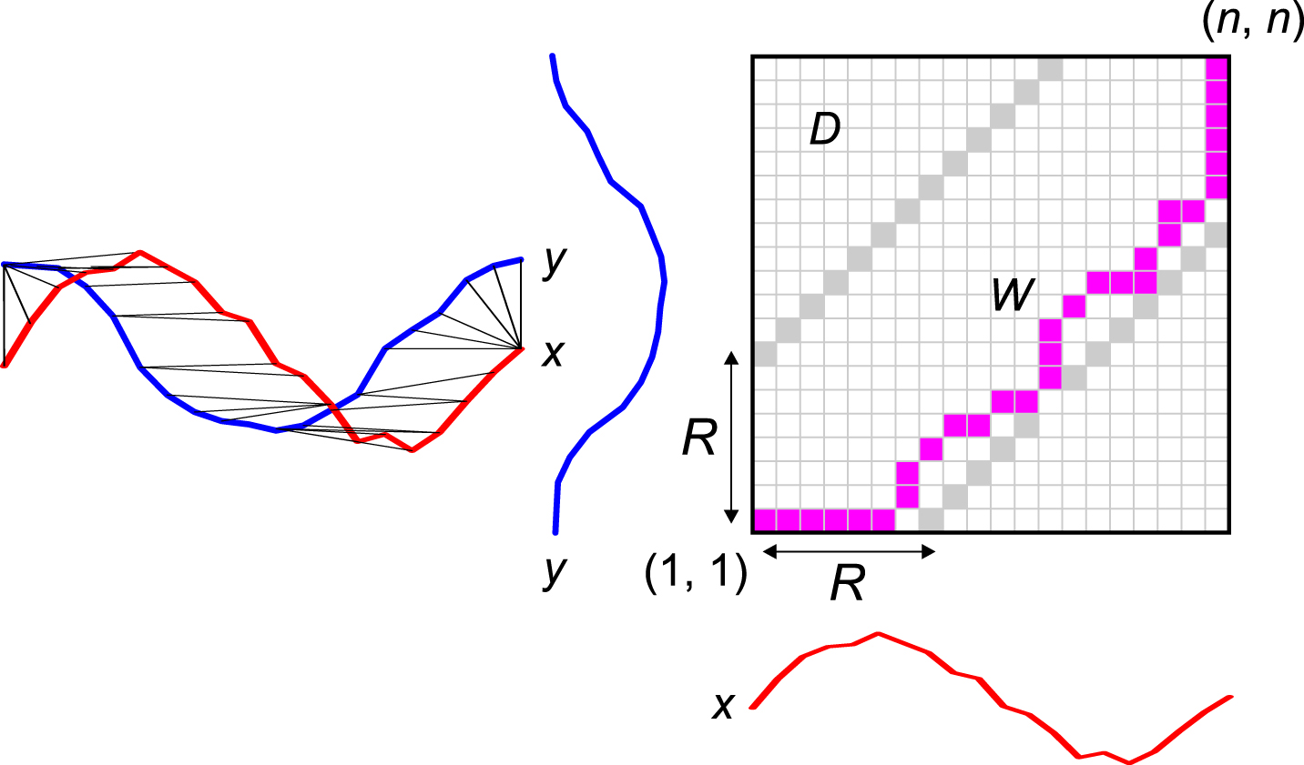
Time series alignment and the corresponding warping path.
The remainder of the paper is organized as follows. Firstly, we give an overview of the dissimilarity measures used (Section 2). The data sets used are described at the beginning of Section 3. Later in that section we describe the experimental setup. The analysis of results is illustrated with tables and figures in Section 4. The same section contains the results of rigorous statistical analysis. We conclude the paper in Section 5.
Classifier
The most popular time series classification method involves the use of a nearest-neighbor-based classifier with various distance measures [34]. The most popular specific method is 1NN-DTW, which is a special case of the k-nearest neighbor classifier with k = 1 and the DTW distance, which demonstrates superior performance for time series classification [4, 31].
Dynamic time warping (DTW)
The Dynamic Time Warping distance measure (DTW) is a very popular and efficient
dissimilarity measure for time series [6]. To
compute the DTW value for two one-dimensional time series with length
n ∈ N
Then we construct a square matrix D with dimensions
n × n containing values of the local cost function
D (i,
j) = d (x (i) ,
y (j)). The matrix element
D (i, j) corresponds to the alignment
between values x (i) and
y (j) of the time series. Then we construct a warping
path W = {w1, w2,
…, w
K
} (K ∈ N) of elements
of the matrix D. For classical DTW the warping path is required to meet
the following criteria: w1 = d (1, 1) and
w
K
= D (n,
n) (boundary conditions), if
w
k
= D (i
k
,
j
k
) and
wk+1 = D (ik+1,
jk+1) then
ik+1 - i
k
≤ 1
and
jk+1 - j
k
≤ 1
(continuity), ik+1 - i
k
≥ 0
and
jk+1 - j
k
≥ 0
(monotonicity).
To obtain a warping path we start from the element D (1, 1) and,
shifting at most one index forward, we end at the element
D (n, n) (Figure 1). The path that minimizes the warping path
gives the value of DTW:
In practice we often compute DTW by building a cumulative distance matrix
Γ. We can use dynamic programming with the following recurrence:
The distance measure DTW does not satisfy the triangle inequality, so it is not a metric. However, it is the case that DTW (x, x) =0 and DTW (x, y) = DTW (y, x) for the cost function (1).
To decrease the computation time and to increase the accuracy of the classification we can use global constraints for distance measures. One of the most popular for DTW and other elastic measures is the Sakoe–Chiba band [30] with radius R (Figure 1). The same technique can be used for the other elastic dissimilarity measures presented below.
DTW
We will use an integer percentage radius r ∈ [0 % , 100 %] with a step
of 1%. Then to obtain the absolute radius R, depending on the length
n of a time series, we compute
To compute DTW we usually use dynamic programming with the following recursion:
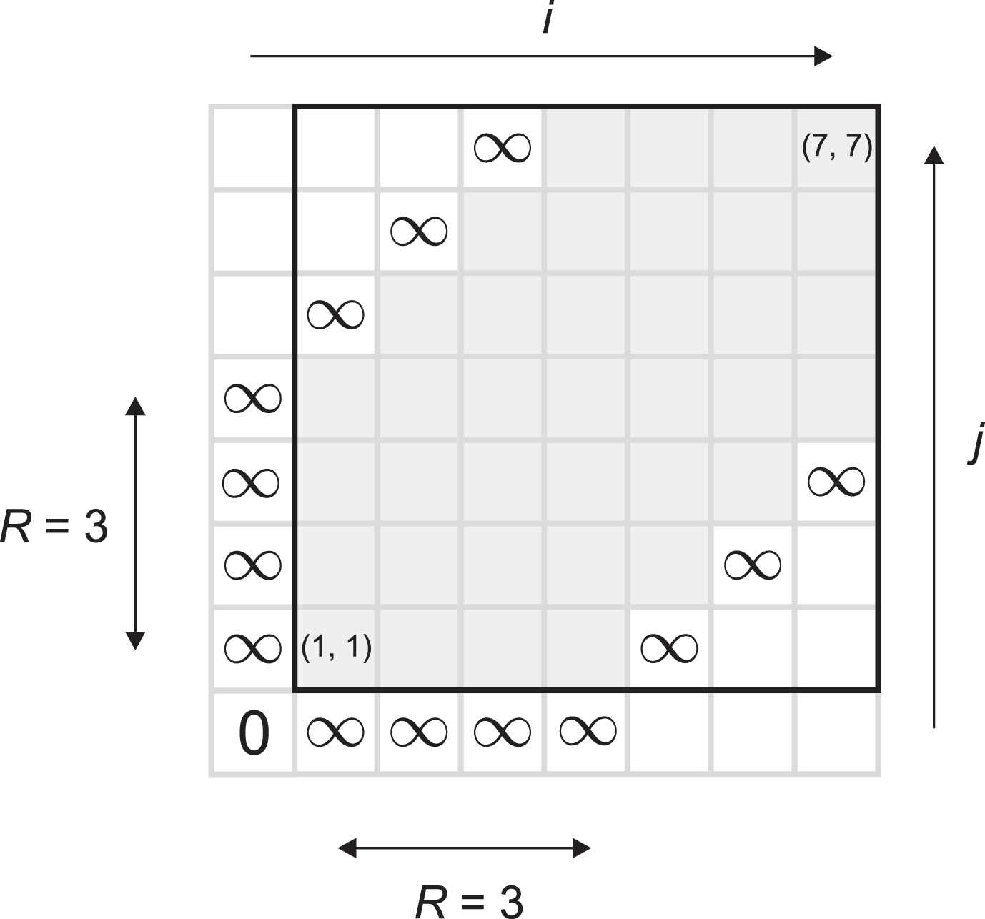
The matrix Γ with initial conditions for DTW.
Then the value of DTW is
The Longest Common Subsequence (LCS) distance measure is based on the edit distance
used for string comparison. It is computed as the longest matching subsequence [32]. The strict string condition
x
i
= y
j
is weakened for time series to
|x
i
- y
j
| ≤ ɛ
with parameter 0 < ɛ < 1. To compute LCS we usually use dynamic
programming with the following recursion:
Then the value of LCS is
ERP
The Edit Distance with Real Penalty (ERP) uses the L1
distance between elements of time series as the penalty for local shifting of time
series [7, 8]. ERP is used in many areas of classification and clustering of time series
data [27, 35]. To compute ERP we usually use dynamic programming with the following
recursion:
EDR
The Edit Distance on Real sequence (EDR) is a variation of the edit distance that finds
the minimal number of edit operations to convert one time series to another [1, 8].
The strict condition
x
i
= y
j
is weakened for time series to
|x
i
- y
j
| ≤ ɛ
with parameter 0 < ɛ < 1. To compute EDR we usually use dynamic
programming with the following recursion:
Then the value of EDR is
Distance measures with derivatives
We will also examine two distance measures based on derivatives with global constraints of radius r.
DDTW
Derivative Dynamic Time Warping [20] is the
DTW distance measure computed on the data transformed by the first (discrete)
derivative:
Then we can simply compute the value of DDTW with radius r by:
DDDTW
Parametric Derivative Dynamic Time Warping was introduced in [16] and examined in several papers [15, 25]. It is a convex combination of the distances DTW and DDTW:
where α ∈ [0, 1] is a parameter chosen in the learning phase of the classification. To obtain a constrained version of DDDTW with radius r we use DTW and DDTW (Sections 2.3.1 and 2.4.1) with the same radius r.
Data sets and experimental setup
We performed experiments on 85 data sets from the UCR Time Series Classification Archive [9]. This is a database with labeled time series data from a very broad range of fields, including medicine, finance, multimedia and engineering. Each data set from the database is split into training and testing subsets. All time series instances are z-normalized.
Constrained versions (with radius r) of the following elastic distance measures were used in the experiments: DTW, LCS, ERP, EDR, DDTW, and DDDTW. For LCS and EDR the parameter ɛ was fixed at the value ɛ = 0.25.
For the classification process the nearest neighbor method (1NN) is used for all of the compared distance measures. We use the cross-validation (leave-one-out) method to find the best r value on the training subset, where r ∈ [0, 100] with a step of 1. If there is more than one optimal value of r, we may choose the minimum, median or maximum of those values. These three methods of tie-breaking are analyzed in the results of the experiments. We study two different strategies for selecting the best value of the radius r. First, we try to fix the same perfect value of the r parameter for all data sets. Second, we try to select the best value for each data set separately, from 0 to a fixed rmax.
For the parametric distance DDDTW a finite subset of values of the parameter α is considered, ranging from 0 to 1 with a fixed step size of 0.01. This means that, for the fixed r, we find the best α by leave-one-out cross-validation on the learning subset.
Results
Methods of tie-breaking
We find a set of radii r with the same minimal error on the training subset. Then we examine three methods of tie-breaking by choosing the minimal, median, or maximal r and computing the error on the test subset.
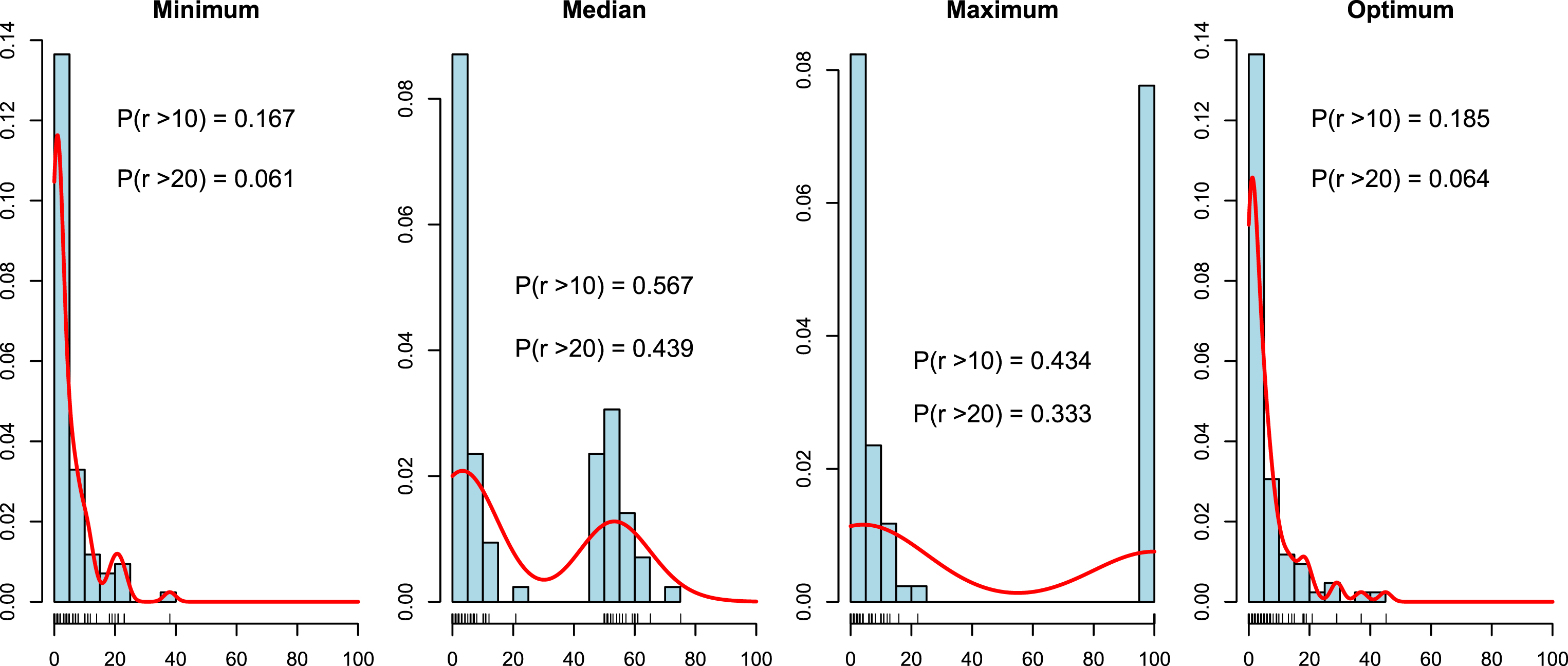
In the first step we decided to create histograms of r (selected by the leave-one-out method on the training data set) for different methods of tie-breaking and different dissimilarity measures (Figures 3–8). We also include a non-parametric estimate of the density of r. Additionally, in each figure we have added the probabilities that r is greater than 10% and 20%. For each dissimilarity measure we have four plots, with three methods of tie-breaking and the optimum value of the parameter r found on the test data set. We would like to find the tie-breaking method which gives us the true value of the parameter r.
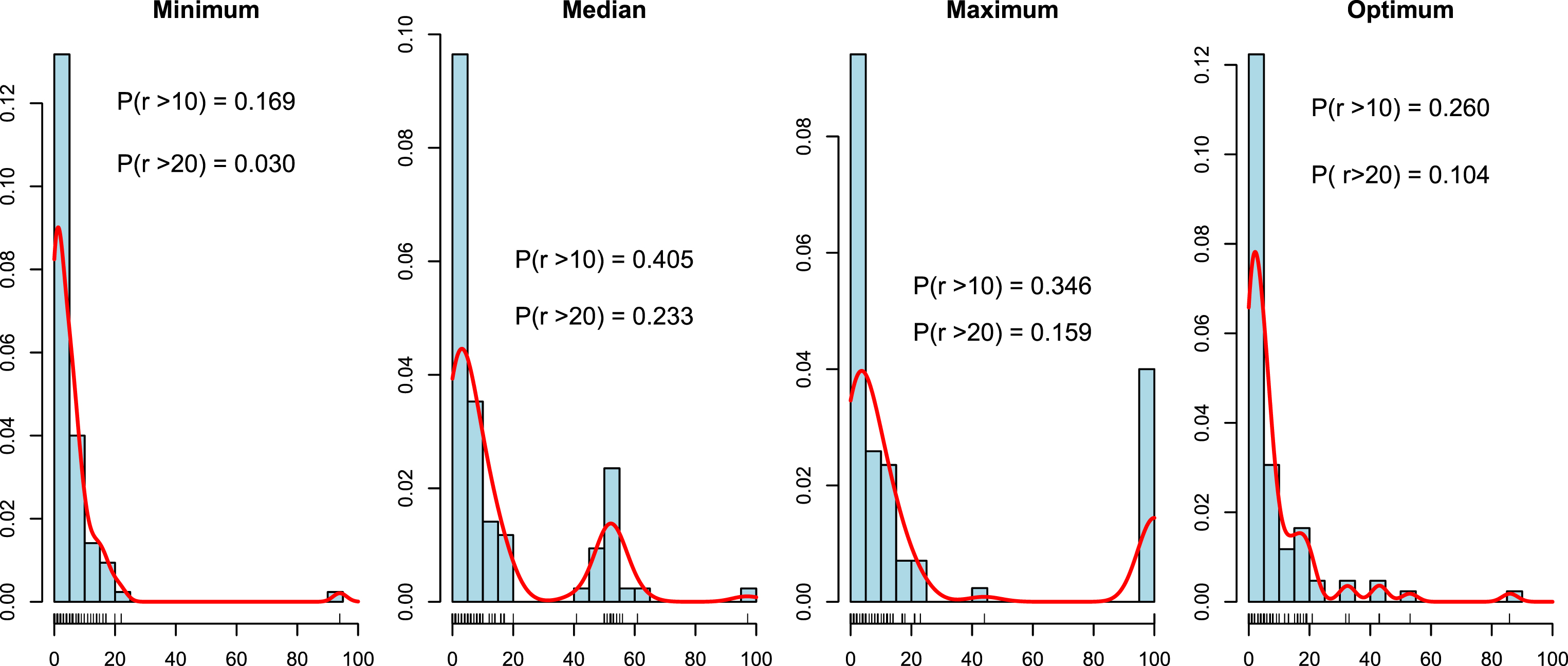
Histograms and densities of r for tie-breaking methods for DTW distance.
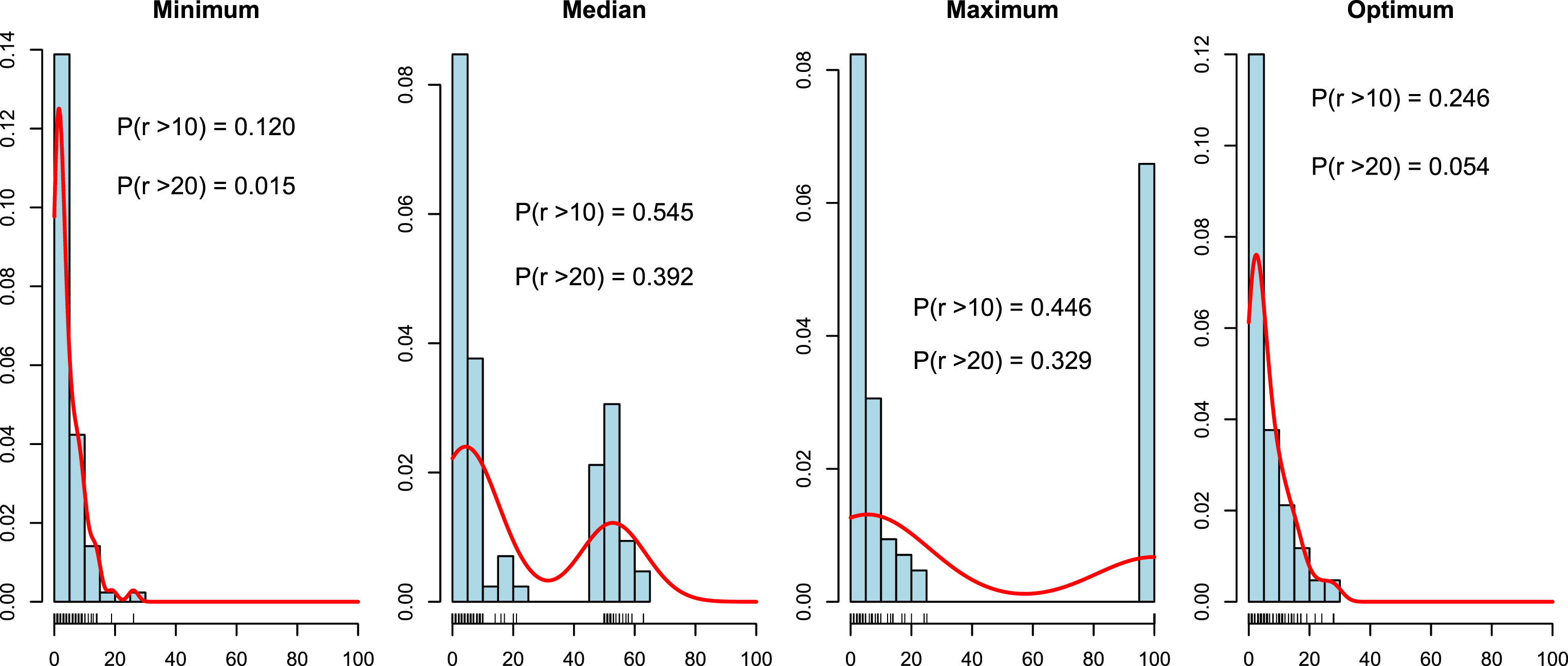
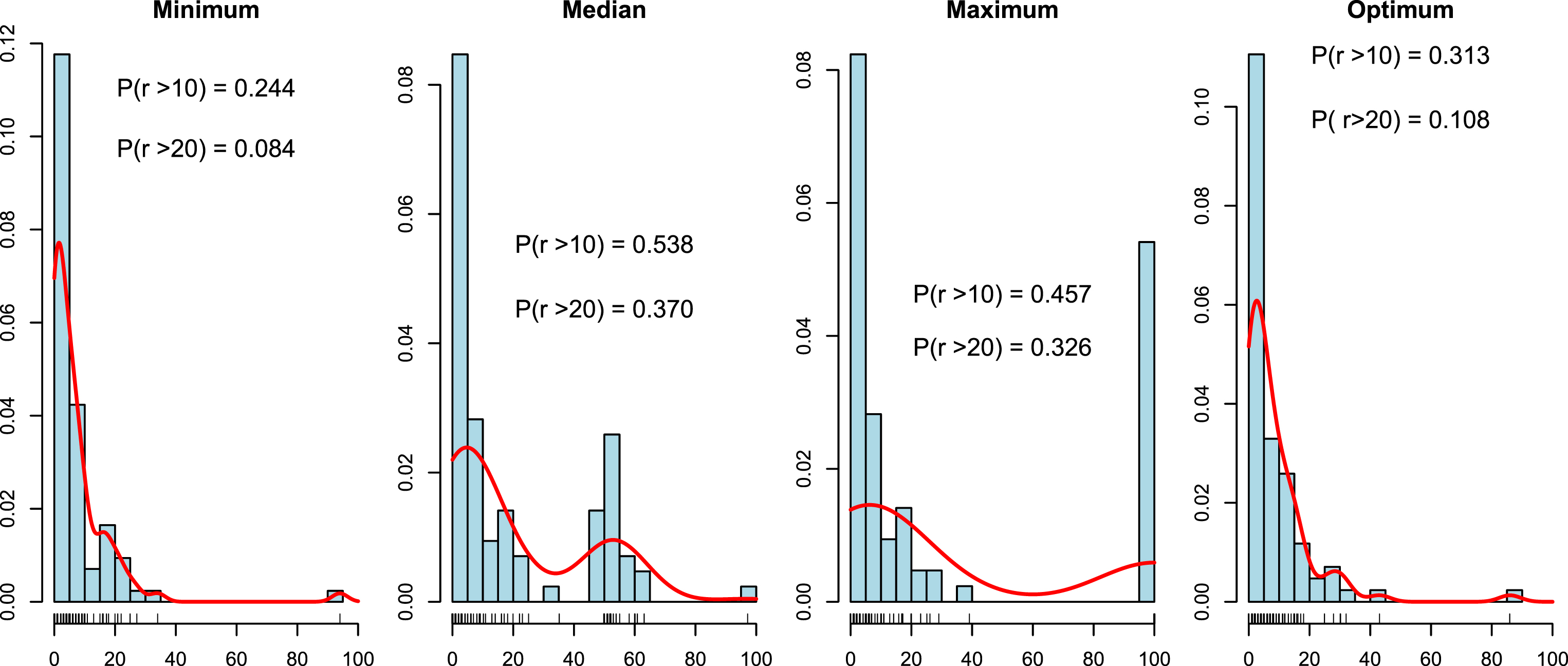
Histograms and densities of r for tie-breaking methods for LCS distance.
Histograms and densities of r for tie-breaking methods for ERP distance.

Histograms and densities of r for tie-breaking methods for EDR distance.

Histograms and densities of r for tie-breaking methods for DDTW distance.
Histograms and densities of r for tie-breaking methods for DDDTW distance.
We can observe that for each dissimilarity measure the histogram of the “Minimum” method looks the most similar to that of the “Optimum” method. For the “Median” method of tie-breaking we notice a high peak in the middle of the distribution of r. This peak is not observed for the “Optimum” method. Similar behavior can be observed for the “Maximum” method. In this case the peak is at the end of the distribution. The probability P (r > 10) is less than 30% and P (r > 20) is less than 10% for the perfect value of r. The “Minimum” method approximates this probabilities quite well (it is definitively the best method) for each dissimilarity measure. Hence, looking at the densities we can recommend the “Minimum” method of tie-breaking. Additionally, it seems that r less than 20% is sufficient for most of the data sets.
Finally, to distinguish statistically the methods of tie-breaking for each distance
measure, we performed a detailed statistical comparison. We tested the hypothesis that
there are no differences between tie-breaking methods. We used the [18] test, which is a less conservative variant of the Friedman’s
repeated-measures ANOVA. This test is recommended by [11, 13] as the best test to compare
several different classifiers. In this test we rank the classifiers for each data set
separately. Let R
ij
be the rank of the
jth of K methods on the ith of
N data sets and let
P-values from the Iman & Davenport test for tie-breaking methods
Fixed r
The first way to choose the radius r is to fix the same
r for all data sets. We try to find an r which is
statistically better (higher rank, lower error) than the full radius
r = 100. To test this statistically we used the [18] test, introduced earlier. For each comparison we obtained
p-values equal to 0. In such a case we should apply a post hoc test to discover the
structure of groups of similar radii. The test statistic for comparing the
ith and jth algorithm is
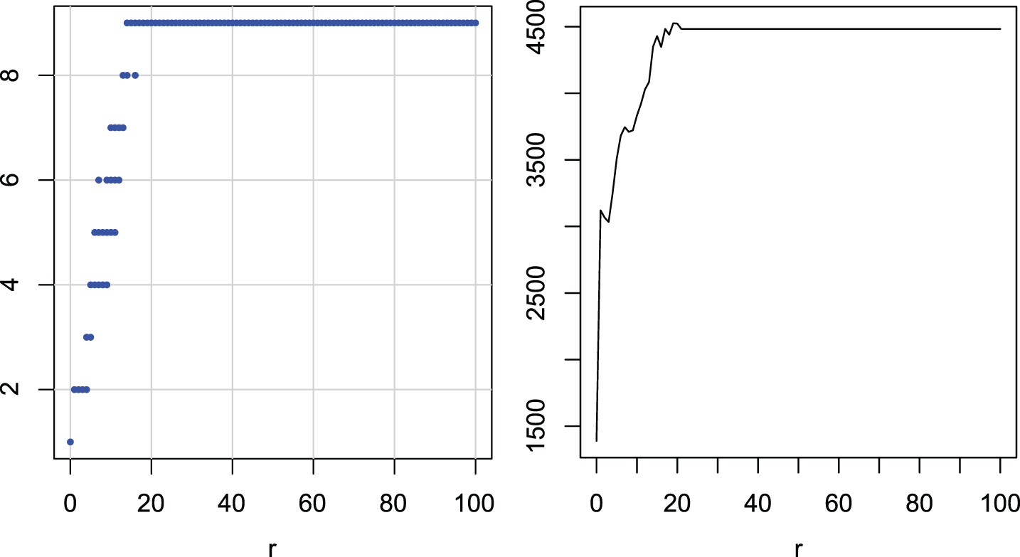
In Figures 9–14 we have groups of radii with similar ranks (left) and values of the rank depending on r (right). Each group is statistically separated from the others. Using these graphs we can see which r is the best for which distance measure.
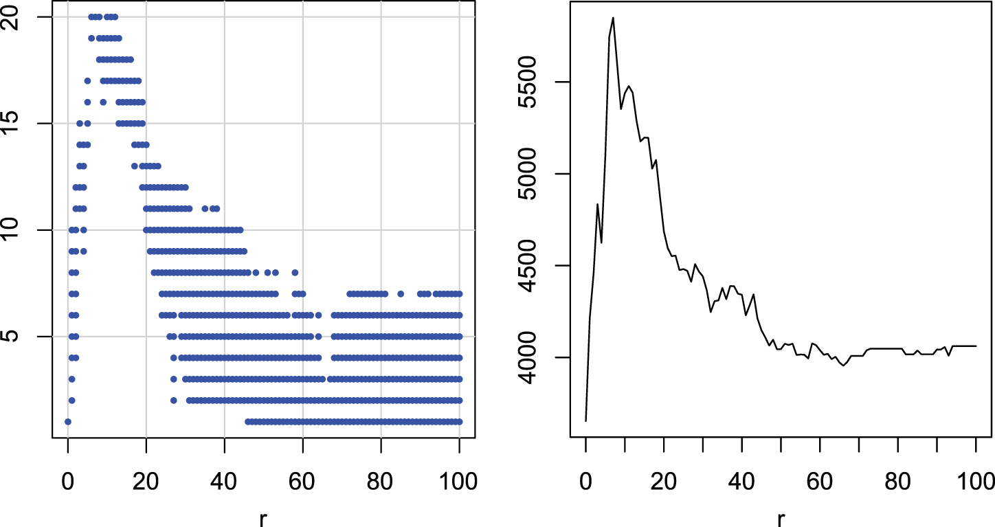
Multiple comparisons of radii r for DTW. Groups of radii with similar ranks (left). Ranks of radii (right).
Figure 9 shows the groups and ranks for DTW. We can see that the best group, with the highest ranks and the lowest errors, is the interval [6, 12]. The group is clearly separated from all groups with r = 100 included. A value of r around 10 seems to be the best choice in this case.
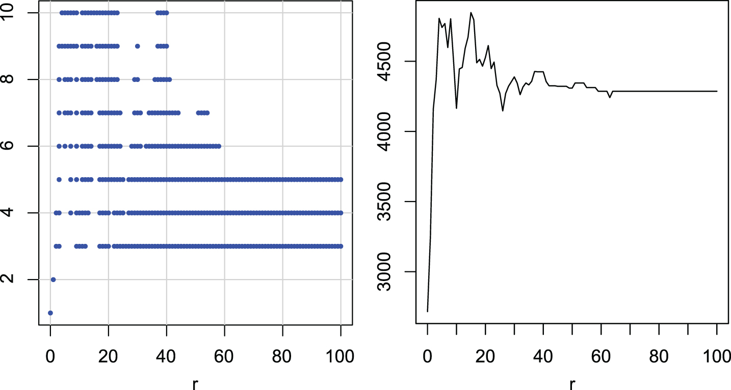
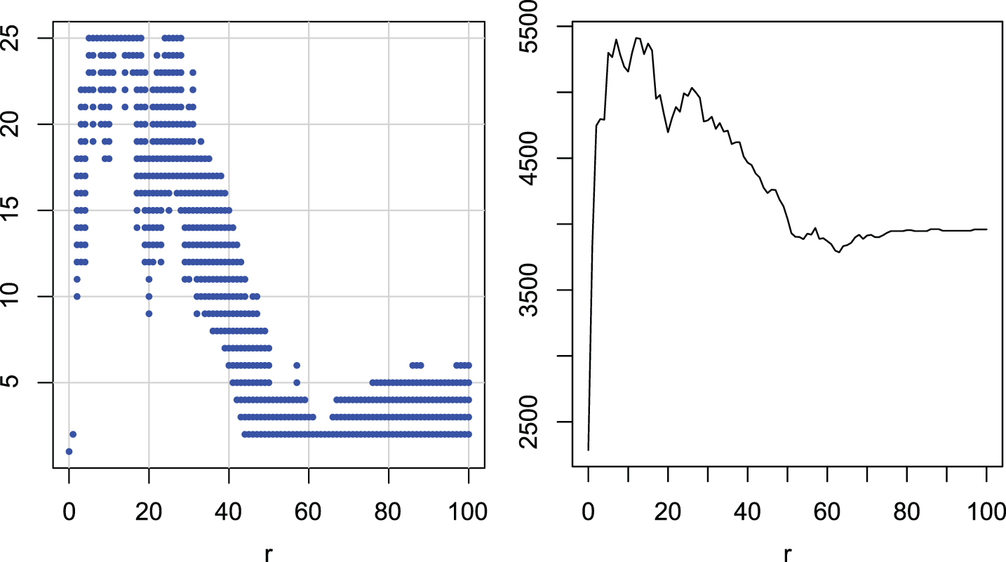
Figure 10 shows the groups and ranks for LCS. The best group is the interval [7, 20] (with a few values excluded). In this case the best group is not separated from the groups with r = 100. Only the values r = 13, 15, 16 are not included in other groups with r = 100. Therefore we can only say that values of r around 15 give results not worse than other radii including the full radius r = 100.

Multiple comparisons of radii r for LCS. Groups of radii with similar ranks (left). Ranks of radii (right).
Figure 11 shows the groups and ranks for ERP. There is a fairly wide group with the highest ranks, but only a few radii are excluded from the groups with r = 100. Values of r from around 5 to around 20 give the same and sometimes better results than r = 100. It seems that a value of around r = 10 is a good choice in this case.
Multiple comparisons of radii r for ERP. Groups of radii with similar ranks (left). Ranks of radii (right).
Figure 12 shows the groups and ranks for EDR. The graph is very clear: there is one very wide group that includes all values of r from 14 to 100. Since as usual the smallest r is preferred, a value around 15 is the best choice.
Multiple comparisons of radii r for EDR. Groups of radii with similar ranks (left). Ranks of radii (right).
Figure 13 shows the groups and ranks for DDTW. The continuous group with the highest ranks is the interval [5, 18], which is clearly separated from the groups with r = 100. Moreover, r = 12, 13 belong only to the best group. It seems that values from around 10 to 15 are the best choice.
Multiple comparisons of radii r for DDTW. Groups of radii with similar ranks (left). Ranks of radii (right).
Figure 14 shows the groups and ranks for DDDDTW. The group with the lowest errors is the interval [7, 17], where radii from 7 to 12 are not included in groups with r = 100. The value r = 11 belongs only to the best group. It seems that r around 10 is the best choice.

Multiple comparisons of radii r for DDDTW. Groups of radii with similar ranks (left). Ranks of radii (right).
The second way to choose a radius r is to fix a maximal radius rmax and find the best r in the interval [0, rmax]. We find the best r (with the smallest error) on the training subset using the leave-one-out cross-validation method. To statistically test algorithms for different radii we used the methodology described above.
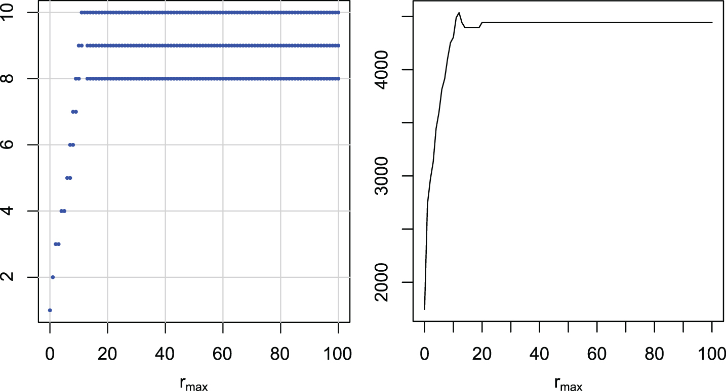
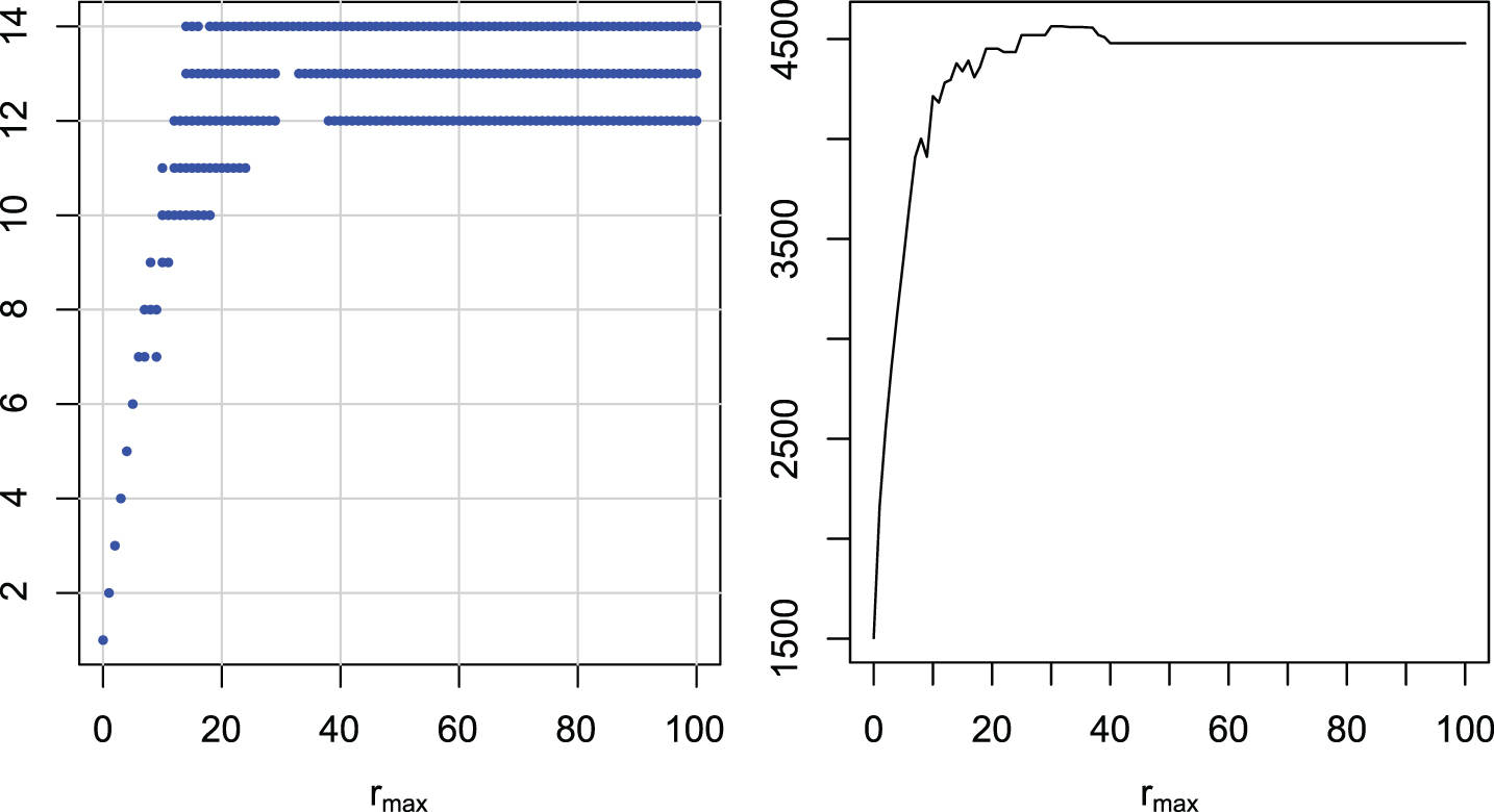
In Figures 15–20 we have groups of maximal radii with similar ranks (left) and values of the rank depending on rmax (right). Each group is statistically separated from the others. Using these graphs we can see which rmax is the best for which distance measure.
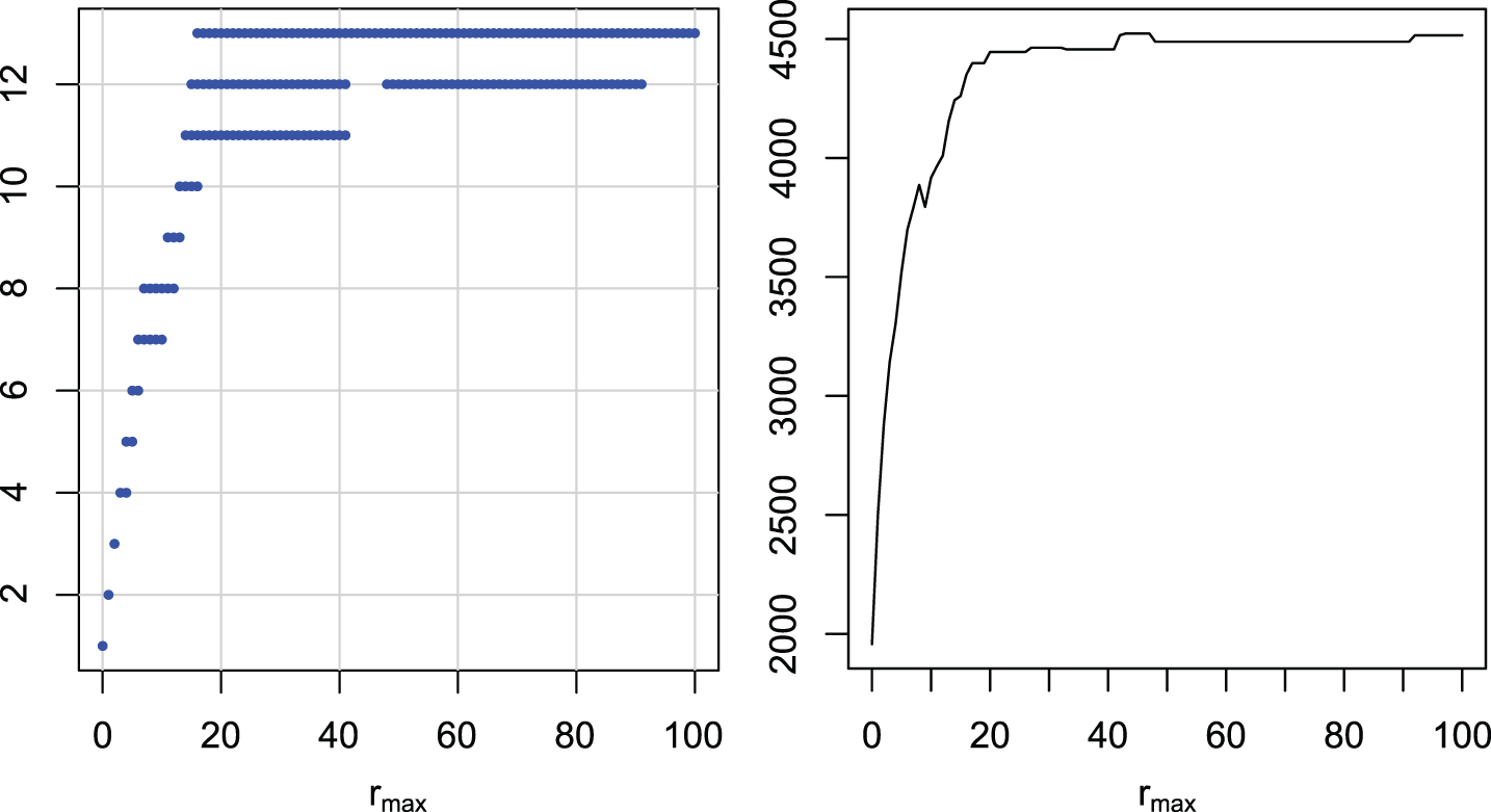
Multiple comparisons of maximal radii rmax for DTW. Groups of maximal radii with similar ranks (left). Ranks of maximal radii (right).

Multiple comparisons of maximal radii rmax for LCS. Groups of maximal radii with similar ranks (left). Ranks of maximal radii (right).
Multiple comparisons of maximal radii rmax for ERP. Groups of maximal radii with similar ranks (left). Ranks of maximal radii (right).
Multiple comparisons of maximal radii rmax for EDR. Groups of maximal radii with similar ranks (left). Ranks of maximal radii (right).
Multiple comparisons of maximal radii rmax for DDTW. Groups of maximal radii with similar ranks (left). Ranks of maximal radii (right).

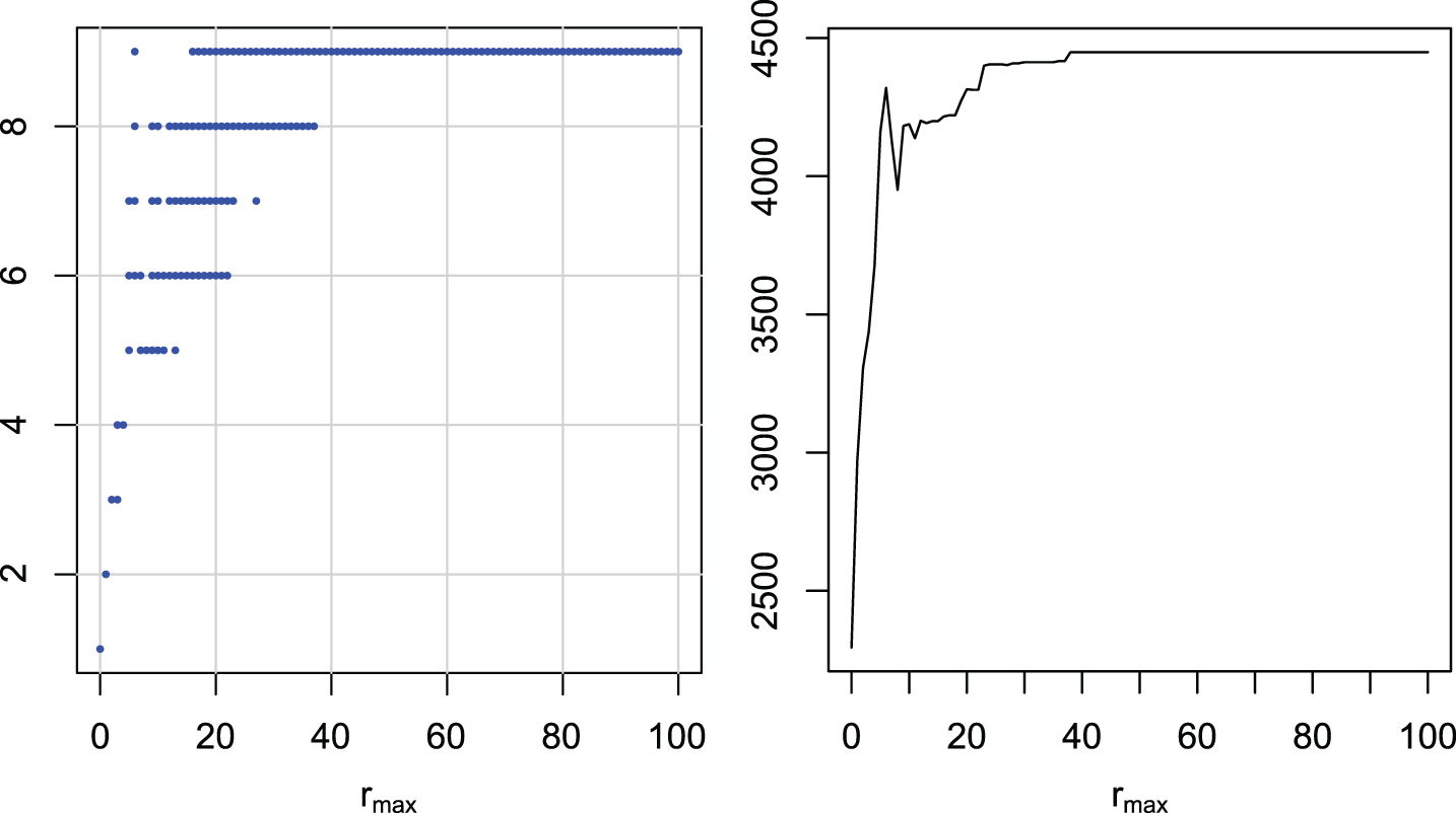
Multiple comparisons of maximal radii rmax for DDDTW. Groups of maximal radii with similar ranks (left). Ranks of maximal radii (right).
The graphs are similar for all distance measures. There is one wide group including rmax = 100 with the highest ranks, and there is no better group. The best groups start with the maximal radius: 16 for DTW, 13 for LCS, 16 (6) for ERP, 11 for EDR, 14 for DDTW, and 12 for DDDTW. If we have to take one universal rmax for all of the examined distances, a value around 20 seems to be the best choice.
We compared a fixed choice of r with the method of finding the best r from 0 to rmax. For every distance measure we take the minimal r and the minimal rmax from the best group (Table 2).
Lowest r and rmax in the best group,
p-values of the Wilcoxon test, and win/tie/loss numbers
Lowest r and rmax in the best group, p-values of the Wilcoxon test, and win/tie/loss numbers
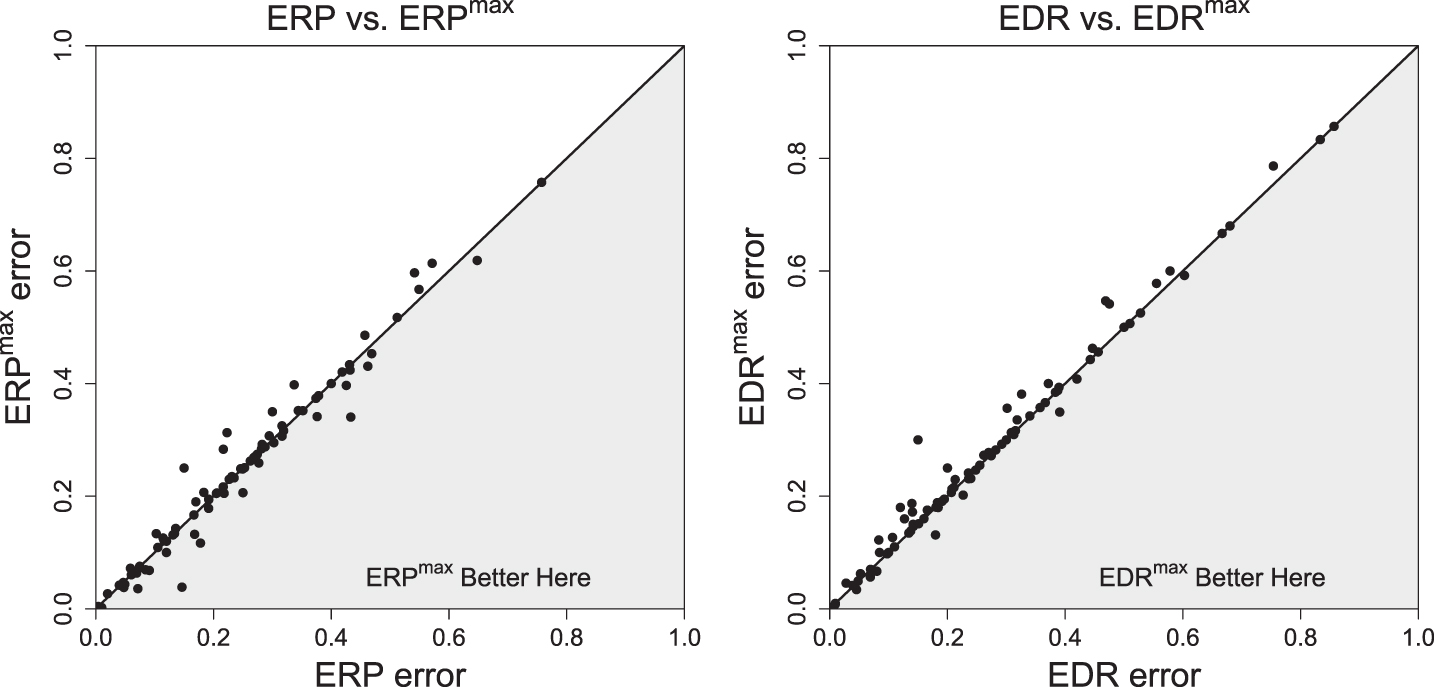
As a first step we decided to prepare a graphical comparison of methods (Figures 21–23).
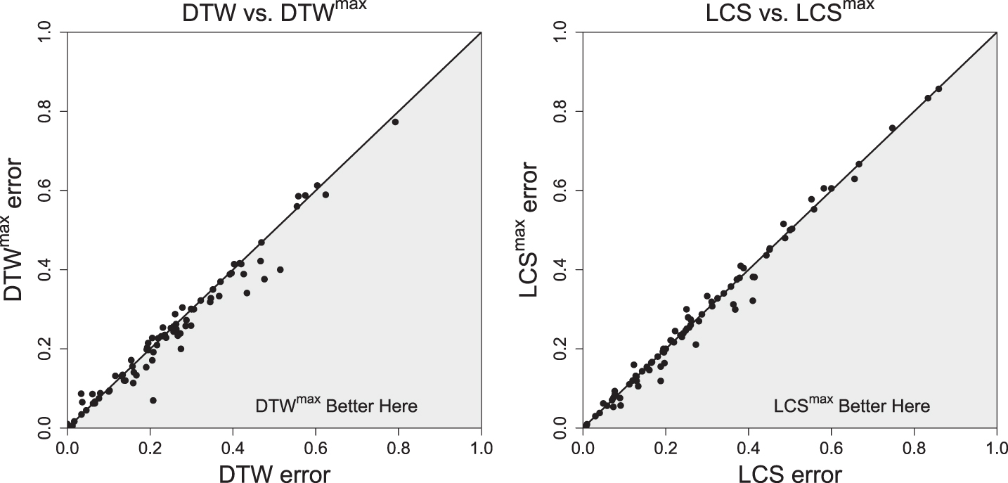
Comparison of test errors.
Comparison of test errors.
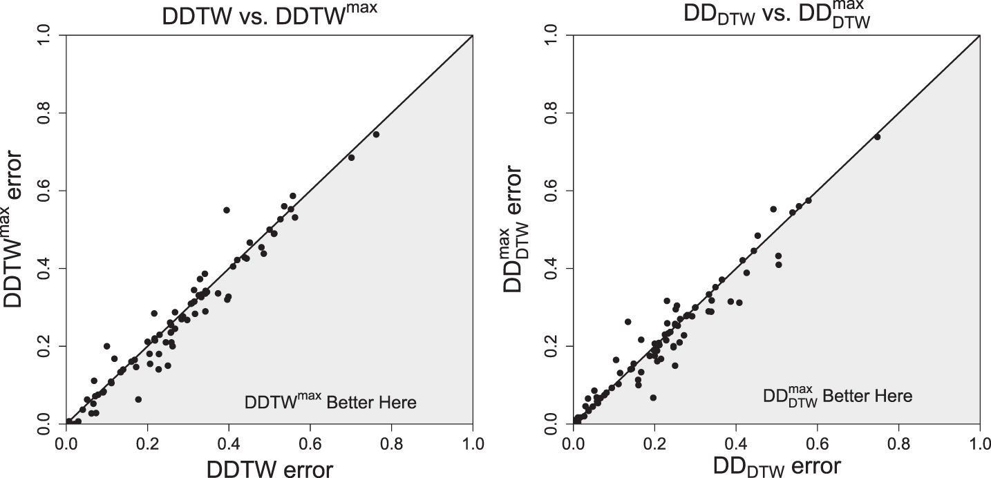
Comparison of test errors.
Finally, we present a statistical comparison. To statistically compare two classifiers over multiple data sets, [11] recommends the Wilcoxon signed-ranks test, which is a non-parametric alternative to the paired t-test. The obtained p-values and numbers of wins/ties/losses are presented in Table 2. As we can see, the p-values and W/T/L numbers show that for distances LCS, ERP, and DDDTW the methods with fixed r and with tuned r ∈ [0, rmax] are statistically the same. For DTW and DDTW the rmax method is better than for fixed r. The only case for which fixed r method is better than the tuned rmax method is that of the EDR distance measure. The graphical comparison in Figures 21–23 confirms the results.
First, we sum up the results concerning tie-breaking methods for finding r on a training subset with leave-one-out cross-validation. Both the analysis of probability distributions of r (Figures 3–8) and statistical tests show that the proposed methods of choosing r are statistically indistinguishable. Since the value of r has a significant influence on the computational complexity of the distance measures, the best choice is the minimal r for all studied distances.
Next, we tested whether for the fixed r method we can take r < 100 with the same or better result than for r = 100. It turned out that the minimal r values in the best group (with highest ranks/lowest classification errors) are very small and are lower than 10 for all of the distance measures except of EDR (Table 2). Furthermore, for all distances, these minimal radii give better (the same in the case of EDR) results (lower classification errors) than r = 100. This shows that by fixing these minimal r we can greatly reduce the computational complexity of the distances. For example, if we take approximately r = 10, then because the computational complexity of all distances is r2, we have a 100-fold reduction in computational time for all distance measures.
On the other hand, in the case of selecting the best r ∈ [0, rmax], there is no better group than that with rmax = 100. However, the minimal values of rmax in these groups are still much lower than rmax = 100 (Table 2). It seems that a universal value of rmax for all of the examined distance measures may be rmax = 20. Since we select r by the leave-one-out method, we can also achieve large reduction in computational time. Finally, we tested whether the method of choosing the best r ∈ [0, rmax] always gives the better result than the method with fixed r. For DTW and DDTW choosing r on the training subset gives a much better result than for fixed r, while for LCS, ERP, and DDDTW the two methods are statistically the same. For EDR the fixed r was even better than the method with choice of the best r; the reason for this behavior may lie in the weak correspondence of the error rates on the learning (cross-validation) and testing subsets.
In summary: When we have many r with the same error rate on the training subset
we select the minimal one. In the method with fixed r, the standard maximal value
r = 100 represents a significant waste of computing power. Table 2 shows the minimal values
of r that we can select in the best groups for each distance measure.
For all distances these minimal values of r guarantee results not
worse than for r = 100, and sometimes much better. To allow for
scaling for new data sets we can select values of r slightly higher
than the minimal ones. It seems that a recommended universal value for of the all
examined distance measures (excluding the case of EDR) may be r = 10
(r = 15 for EDR). For the method of selecting the best r ∈ [0,
rmax], although we do not have better results than for
rmax = 100, the group with
rmax = 100 is always very wide and the minimal value of
rmax in this group is very low (Table 2). It seems that the value
rmax = 20 is a good choice for all of the examined
distance measures. In accordance with intuition, the method of selecting r ∈ [0,
rmax] is not worse than the method with fixed
r (excluding the case of EDR). For DTW and DDTW we substantially
increase the quality of classification by choosing the best r ∈ [0,
rmax] instead of fixed r. For other
distance measures the results are not conclusive. The special case of EDR seems to be
explained by overfitting—the weak correspondence of the choices of best
r on the training and testing data sets for this distance
measure.