Large-scale dynamic social data representation for structure feature learning

Abstract

The problems caused by network dimension disasters and computational complexity have become an important issue to be solved in the field of social network research. The existing methods for network feature learning are mostly based on static and small-scale assumptions, and there is no modified learning for the unique attributes of social networks. Therefore, existing learning methods cannot adapt to the dynamic and large-scale of current social networks. Even super large scale and other features. This paper mainly studies the feature representation learning of large-scale dynamic social network structure. In this paper, the positive and negative damping sampling of network nodes in different classes is carried out, and the dynamic feature learning method for newly added nodes is constructed, which makes the model feasible for the extraction of structural features of large-scale social networks in the process of dynamic change. The obtained node feature representation has better dynamic robustness. By selecting the real datasets of three large-scale dynamic social networks and the experiments of dynamic link prediction in social networks, it is found that DNPS has achieved a large performance improvement over the benchmark model in terms of prediction accuracy and time efficiency. When the α value is around 0.7, the model effect is optimal.

Keywords

Feature learning social network representation learning neural network

1 Introduction

The network is an important data representation for expressing the relationship between things and things. With the rapid development of information technology, more and more data appear in the form of networks [1]. Analytical methods such as social networks, word co-occurrence networks, bioinformatics networks, communication networks, social structure networks, and other large-scale and complex network structures have attracted increasing attention [2]. Effective network analysis can have a deeper understanding of the knowledge behind the complex network structure, to mine the implicit structural information, different things and different association patterns, so that it plays a key role in many application scenarios [3, 4]. The use of machine learning technology to analyze complex network structure data suffers from insufficient associated information, sparse data, and high computational cost. For the same task on the same data set, different feature representation methods will result in a large performance gap even if the same algorithm is used [5, 6]. Therefore, learning the characteristics of network structure has become a key research task in network analysis research [7]. The network representation learning method expresses network node information and association information between nodes as continuous low-dimensional dense vectors and then inputs them for various tasks, which reduces the computational cost and solves the problem of semantic calculation between heterogeneous objects [8]. The appearance of new content and the disappearance of old content lead to changes in the attribute information carried by some nodes [9]. However, the existing methods are structurally unable to process dynamic information, which prompts us to seek an effective knowledge representation to capture the evolution pattern of network topology and node attribute information and eliminate the noise generated by the original model due to the addition of new information [10]. Also, in most network representation learning work, only the association relationship of directly connected nodes is considered. For nodes that are not directly connected, there is no way to indicate the uncertainty of the relationship between them, it is unable to effectively capture the dependent properties caused by the complex relationship between nodes [11]. Moreover, the existing network representation model considering additional information generally considers the additional information of a single source. For the multi-source and multi-dimensional additional information, it is difficult for the model to obtain an effective joint vector representation due to the inconsistency of the geometric representation and acquisition mode of the information representation [12].

Lei proposed a Bayesian network structure learning algorithm based on an improved particle swarm optimization algorithm. The algorithm is based on the optimization and feature analysis of the particle swarm optimization algorithm. The function of the algorithm is to evaluate the Bayesian network structure in the algorithm. The optimal particles will be preserved during this process and the mutation operation will be used to reduce the likelihood of local optimal solutions. In his simulation, the scheme is compared with algorithm K2. His experimental results show that there is only one Bayesian network structure obtained by the improved particle swarm optimization algorithm compared with the standard Bayesian network structure of the Asian network. On the reverse edge, the missing edge and redundant edge in the Bayesian structure obtained by MPSO are also less than the missing edge and redundant edge in the Bayesian structure obtained by K2. He concludes that MPSO is better than K2. The improved particle swarm optimization algorithm is feasible for Bayesian network structure learning [13, 14]. Bin believes that traditional Bayesian networks have high computational complexity, and the network structure scoring model has a single feature. Therefore, to make up for the shortcomings of the above methods, he proposed a novel hybrid learning method (DBNCS) based on a dynamic Bayesian network (DBN), which is the first comprehensive score to construct multiple time-delay GRN CS) and DBN models. The DBNCS algorithm first uses the CMI2NI (Network Reasoning Based on Conditional Mutually Exclusive Information) algorithm to learn the network structure configuration file, that is, to construct the search space. Then, use the recursive optimization algorithm (RO) to remove redundant rules, thereby reducing the false positive rate. Second, the network structure outline is decomposed into a group without loss, which can significantly reduce the computational complexity. Finally, the DBN model is used to determine the direction of gene regulation within the group and to find the optimal network structure. The algorithm performance was evaluated by the baseline GRN dataset from the DREAM challenge and the SOS DNA repair network in E. coli and compared to other recent methods. His experimental results prove the rationality of the algorithm design and the excellent performance of GRN [15].

The innovations of this paper are as follows: (1) A dynamic network representation learning method based on correlation walk and space synthesis is proposed. Firstly, the parallel embedded space is generated by the relevant walk sample to represent the newly added information and eliminate the noise, and then the parallel based on the matrix perturbation theory. The embedded space is regarded as a low-dimensional vector representation of the updated network when the perturbation factor is integrated into the original semantic space. The effectiveness of the method is proved by experiments. (2) A multi-source additional information representation method based on Gaussian distribution is proposed. Firstly, the Gaussian distribution is embedded in the node to measure the uncertainty of the degree of node association. Secondly, a model framework that can complement the embedded multi-source additional information is proposed. The embedded spaces are complementarily embedded in a unified space, and the effectiveness of the proposed method is verified by experiments.

2 Data representation method for structural feature learning

2.1 Deep neural network

The most basic component of a neural network is the neuron model, as shown in Fig. 1. In a single neuron model, neurons can receive the output of multiple neurons in other hidden layers, process these outputs, perform related matrix multiplication, and use the activation function to process the values to get a completely new output. This output is also the input to multiple neurons in the next hidden layer. Finally, at the output layer of the neural network we can get the results of the entire neural network, and then get the final output through the processing of softmax and other functions. The calculation process of a neuron can be expressed as:

(1) Perceptron and multi-layer neural network

Fig. 1

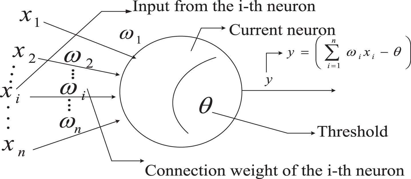
Neuron structure.

The perceptron has only two neural layers, the output layer and the input layer. As shown in Fig. 2, after the input layer obtains the input from the outside world, it undergoes a calculation and passes the result to the output layer. The output layer then performs corresponding calculations to obtain the final result.

Fig. 2

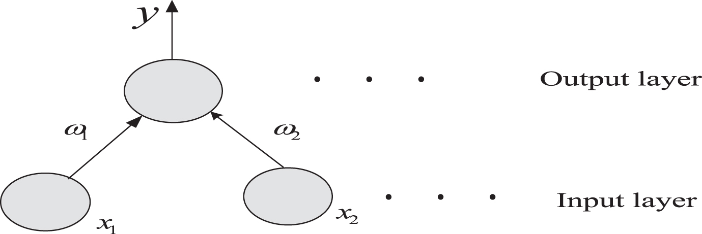
Perceptron structure with two layers of neurons.

The perceptron can easily implement most of the logical calculations, such as calculations, or calculations, and non-computations. However, the perceptron only uses the activation function to convert the output layer neurons, so it is impossible to solve the XOR problem, that is, it is linearly inseparable. To solve the problem of linear indivisibility, it is necessary to consider multi-layer functional neurons, that is, multi-layer neural networks. The structure of multi-layer neural networks is shown in Fig. 3.

Fig. 3

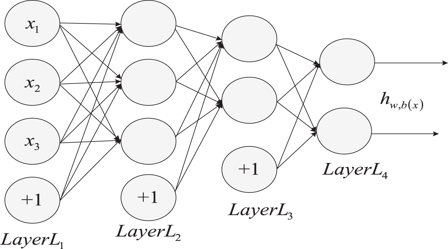
Multilayer neural network structure.

In this model, after the neurons of the input layer obtain the input from the outside world, the result is passed to the hidden layer. The hidden layer and the output layer simultaneously calculate the input, and also use the activation function for processing, and finally the hidden layer. The output is passed to the neurons in the output layer and the result is calculated.

(2) Backpropagation algorithm

The backpropagation algorithm is the core algorithm in the iterative update and correction process of neural network parameters. The principle of backpropagation algorithm backpropagation is very simple, that is, the chain law of derivatives is used: for y = g(x), z = f(g(x))=f(y), there is $\frac{d_{z}}{d_{x}} = \frac{d_{z}}{d_{y}} \frac{d_{y}}{d_{x}}$ (1)

Promoted to the vector form is $\nabla_{x} z = {(\frac{\partial y}{\partial x})}^{T} \nabla_{y} z$ (2)

By using the chain rule, we can continuously derive the gradient of each layer from the final loss function. Backpropagation is a special execution process of chain law operation, which combines dynamic planning to avoid repeated operations for certain operations, in exchange for a faster increase in speed.

(3) Common loss function

The loss function expresses the fit of the model to the data, which is the result of the learning. The lower the value calculated in the loss function, the more the model fits in the training set, and the effect is better. At the same time, when the loss calculated by the loss function is large, the derivative gradient corresponding to each parameter in the network is also large, which can make the parameter update speed faster, to improve the efficiency of model training. The most commonly used loss function is the mean squared loss function. The formula for the mean squared loss function is: $J = \frac{1}{N} \sum_{i = 1}^{N} {(Y_{i} - y_{θ} (x_{i}))}^{2}$ (3)

A recurrent neural network (RNN) can be used to process external inputs of a fixed length and process the sequence data. Ordinary deep neural network inputs are fixed and cannot handle different input lengths. The circulatory neural network solves this problem well. Each output of the recurrent neural network depends on the hidden state produced by the previous input and the current input. The choice of the current output 0 depends on the current input and other inputs previously used. This is why the circulatory nerve is thought to have memory and is the reason why it can process sequence data. The neuron formula of the circulating neural network is as follows: $s^{t} = f (s^{t - 1}; θ)$ (4)

Among them, s^t is called the state of the system.

2.2 Feature learning and recommendation algorithm based on neural network

The development of deep learning provides powerful technical support for feature learning. It combines low-level features to form more abstract deep features to discover effective representations of data. Feature learning based on neural network, through the learning of deep nonlinear network structure to represent a large amount of data related to users and projects, has a powerful ability to learn the essential characteristics of data from the sample. Its main idea is to perform automatic feature learning on multi-source heterogeneous data, map different data to the same hidden space, and obtain a unified data representation. Based on this, it can be recommended in combination with traditional recommendation methods. Utilize multi-source heterogeneous data to effectively address data-sparse and cold-start issues in traditional recommendation systems. The shallow neural network model for feature learning and the commonly used neural network techniques are introduced below.

(1) Embedded representation model

Shallow neural network models, especially embedded representation models, are quickly and relatively effective because they are simple and relatively easy to apply to recommendation systems. The core idea is to construct embedded feature representations of users and projects (or other auxiliary information) at the same time, so that embedded features of multiple entities can share the same hidden space, and then the similarity between two entities can be calculated.

(2) Neural network model

A recommendation system for feature learning using a neural network generally takes various types of auxiliary information related to users and projects as inputs, learns feature representations of users and projects, and represents project recommendations for users based on these features. Also, neural network technologies commonly used in recommendation problems include: Convolutional Neural Network (CNN), Recurrent Neural Network (RNN), and neural networks based on self-Attention mechanism. These neural network technologies can effectively extract the characteristics of users and projects by learning the information from different sources, thus improving the recommendation performance. Combining these technologies with traditional feature learning methods based on collaborative filtering is a hot topic in the field of recommendation systems.

(3) Network feature modeling technology

The training network embedding model node2vec is used to extract the network feature representation of the node. The extraction process generally includes the following three steps: defining a random walk rule for each node according to a given network; performing random walks on the network according to the rules, and saving the walk record. The maximum likelihood function of the walk record is obtained, and the network embedding feature of each node is obtained.

(a) Define random walk rules for each node

Let G=(A; E) be a known network, where A represents a set of nodes and E represents a set of edges. Assume that the last moment of the walk is at node t ∈ A, and now randomly walks to node v ∈ A, then the next step from node v will be to one of the neighbor nodes v′ ∈ A of v, and the probability of π_vv′ is defined as: $π_{{vv}^{'}} = α_{pq (t, v^{'})} = {\begin{matrix} \frac{1}{p}, d_{t, y^{'}} = 0 \\ 1, d_{t, y^{'}} = 1 \\ \frac{1}{q}, d_{t, y^{'}} = 2 \end{matrix}$ (5)

Among them, d_t,v′ refers to the shortest path length of node t and node v′ in the network. In node2vec, p and q are two important parameters, which determine the speed of walking and leaving the neighbor of the starting node. More specifically, the parameter p is a constant that controls the random walk back to the previous node. The high value of p (greater than max(q, 1)) means that we are less likely to sample existing nodes, and the low value of p (less than min(q, 1)) will cause the walk to be close to the starting node. The parameter q is a constant that controls the random walk to select depth traversal or breadth traversal, where the high value of q means that the sample tends to swim toward the node near the starting node, and the low value of q tends to swim away from the starting node.

(b) Randomly walk the network according to the rules and save the travel record.

According to the random walk rule, the user or the project network is obtained, and all nodes in the network are randomly walked with a probability of π and a step length of l, and each time the travel record is placed in the walk list, and the number of loops is set.

(c) Find the maximum likelihood function of the walk record and obtain the network embedding characteristics of each node.

For all nodes in the walk list, the stochastic gradient descent method is used to optimize the function: $max J = \sum_{t = 1}^{T} \sum_{- c ⩽ j ⩽ c, j \neq 0} log p (V_{t + j} | V_{t})$ (6)

Where T is the length of the walk list, c is the window size, and finally the network embedding feature of each node is obtained. To evaluate whether the pre-learned embedded features can better represent users and projects, this paper uses an end-to-end approach to evaluate node2vec by the degree to which the proposed recommendation algorithm can be improved. To find the appropriate parameter settings, we use the grid search method in the experiment, let p, q ∈ {0.25, 0.50, 1, 24} finally, the parameter value which makes the algorithm to achieve the best effect is chosen as the final set.

(4) Introduction to evaluation methods

In this paper, the mean absolute error (MAE) and root mean square error (RMSE) are used to evaluate the recommended performance of the proposed method. The metrics MAE and RMSE are defined as: $MAN = \frac{1}{N} \sum_{u, i} | r_{u, i} - {\hat{r}}_{u, i} |$ (7) $RMSE = \sqrt{\frac{1}{N} \sum_{u, i} {(r_{u, i} - {\hat{r}}_{u, i})}^{2}}$ (8)

Where r_u,i is the actual rating value of user i for item i, and ${\hat{r}}_{u, i}$ is the corresponding predicted rating value? N represents the number of users used for testing. Since MAE and RMSE measure the prediction error of the recommended method, the lower values of MAE and RMSE indicate that the method can be predicted more accurately.

This paper evaluates the recommended performance of the proposed method by two widely used indicators, Precision@k and Recall@k. The formulas for Precision@k and Recall@k are defined as follows: $Pr ecision @ K = \frac{1}{N} \sum_{u = 1}^{N} \frac{| L^{k} (u) \cap L^{T} (u) |}{K}$ (9) $Re call @ K = \frac{1}{N} \sum_{u = 1}^{N} \frac{| L^{k} (u) \cap L^{T} (u) |}{| L^{T} (u) |}$ (10)

Where N is the number of users, L^T (u) represents the set of locations that user u has visited in the test data, L^k (u) represents the top k POI sets recommended by user u, and k is the length of the recommended list.

3 Simulation analysis of data representation method for structural feature learning

3.1 Experimental design

The main settings of the unified experimental environment for all models (including comparative models) are shown in Table 1. The common hyperparameters of all models in the experiment follow the principle of unified control variables. By setting the benchmark parameters, the accuracy and time efficiency of different models are compared and analyzed in the same framework. In the experimental analysis section, the effect of the model (or comparison model) and the influence of its hyperparameters will be further elaborated.

Table 1
Experimental system setup information

Project Setting Quantity

Operating system Yosemite 10.10.5 1

CPU Intel i7-5280k,6 cores,12 threads 1

Hard disk 512GB PLEXTOR PX-512M6Pro SSD 1

RAM Kingston 8GB DDR4 2400 8

Important package Python2.7.11, Cython0.23.4 1

Project	Setting	Quantity
Operating system	Yosemite 10.10.5	1
CPU	Intel i7-5280k,6 cores,12 threads	1
Hard disk	512GB PLEXTOR PX-512M6Pro SSD	1
RAM	Kingston 8GB DDR4 2400	8
Important package	Python2.7.11, Cython0.23.4	1

To verify the validity of our proposed method, this paper compares the recommended results with the following methods:

MostPopular, which is a simple but effective recommendation method, is designed to recommend the most visited POI to each user.

LRT, a time-aware POI recommendation method, explores the impact of temporal features on recommendation performance by modeling user preferences over different periods.

MGMPFM, a hybrid model that combines geographic and social influences with matrix decomposition, assumes that user sign-in probability is consistent with a multi-center Gaussian model.

iGSLR, a personalized, unified recommendation framework that combines user preferences, social impact and geographic impact, using a nuclear density estimation approach to personally model the geographic factors of user sign-in behavior.

BPRMF, an efficient way to handle implicit feedback, uses Bayesian criteria to directly optimize individualized sorting.

WMF, another advanced recommendation for solving implicit feedback problems, assigns a smaller weight to the negative instance of the sample.

The experiments in this section divide each data set into three separate parts, the training set, the tuning set, and the test set. Specifically, select the earliest 70% of the behavior data (70% of users – POI pairs) for each user, and the last 20% of the check-ins as test data, and adjust the parameter values, so that the remaining 10% of the data is reached the best result under the algorithm. The experimental parameters of the method L-WMF are set as follows: For Gowalla, the geo-regularization parameter λ_T is set to 0.0001 and the parameter α is set to 15. For Foursquare, set λ_T to 0.00002 and α to 20. For Gowalla and Foursquare, the dimension D of the potential factors U and V is set to 10, and the regularization parameters of U and V are set to λu = λv = 0.005.

3.2 Data collection

Considering the analysis of the dynamic process of social networks, we need to select the social network dataset with timestamp. Therefore, we have selected three large-scale dynamic network datasets that are widely used: A network, B network and C network. The above three networks are calculated in units of “days”, and the number of newly added edges is calculated to obtain the new side frequency distribution of the network. In the process of cleaning and counting the data sets, we find that the original collectors are in the data. There is a gap in the acquisition process, that is, it is not a complete sampling. For example, the C network dataset collects network dynamic changes from January 1, 2017 to the end of December 25, 2018, where each acquisition interval is 1 day. Because both B and C network datasets exist “Stop” situation, therefore, we use the equal-length date as the partition for the dynamic link prediction problem of the above data set.

3.3 Network structure feature representation learning experiment analysis

(1) Analysis of the influence of dimensions on model effects.

The network learning representation model based on node location information and converged network structure involves many parameters. Among them, the parameters common to DeepWalk and node2vec include the dimension of the representation, the length of the sliding window, the length of the random walk sequence, the number of random walk sequences selected for each node, etc. Also, node2vec involves two parameters that control the sampling range. The same parameters of LINE and SDEI include the dimensions of the representation, the learning rate, etc., and the SDEE also relates to the coefficient terms of the first-order and second-order similarity loss functions. In summary, the common parameters in the two types of models are only the dimension d of the network representation. Therefore, this section will explore the effect of the dimension selection of the fusion model on the effect of link prediction.

As shown in Fig. 4, the effects of the integrated model in different dimensions are shown. As can be seen from the figure, at the beginning, as the dimension increases, the effect of the model increases. This is because the higher the dimension of the vector, means that more useful network structure information is encoded into the vector. When the dimension reaches 256, the model effect reaches the highest value, and then decreases with the increase of the dimension. The possible reasons for this phenomenon include two aspects: on the one hand, the high dimension introduces noise, which has an impact on the model effect; On the one hand, in the logical classifier, the dimension represented by the network is the vector dimension of the input feature space. Excessive feature dimension confuses the learning algorithm and leads to the over-fitting problem of the classifier, that is, the classifier is too complicated. Its performance is declining. From the trend of the curve, the change of the integrated model in the dimension is consistent with the single model. Experiments show that choosing the appropriate spatial representation of the network dimension is important to the performance of the model.

Fig. 4

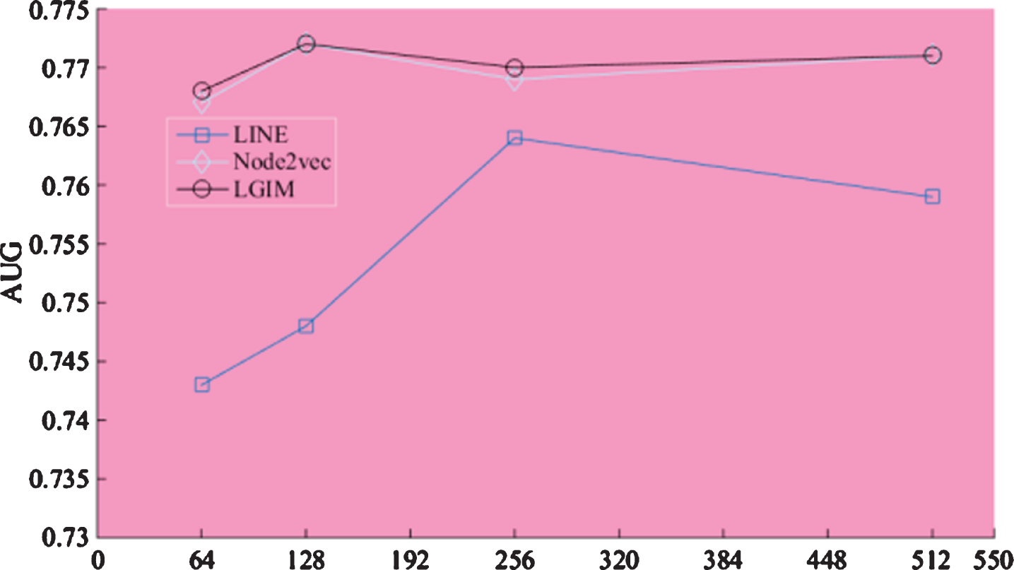
Effect of dimensions on model effects.

(2) Analysis of the influence of fusion parameters on the model effect

The fusion parameters in the integration model are adjusted, and the results are shown in Fig. 5. In the figure, the fusion ratio α of the node2vec model is the abscissa and the AUC value is the ordinate. When α=0, it means that only a single LINE model is included; when α=1, it means that only a single node2vec model is included. It can be seen that when using a single model for link prediction, the effect of node2vec is better than that of the LINE model; on the training sets of different scales, the effect curve of the model as a whole has an inverted “U” shape distribution, and with the increase of α, the effect of the integrated model gradually moves towards the single model with better effect. When α reaches the optimal certain value, the model effect is optimal, and then it shows a weak downward trend. For example, using the financial domain dataset training model, as shown in Fig. 5, the effect of the integrated model is significantly better than the single model. When the alpha value is around 0.7, the model effect is optimal. The experimental results illustrate the following two conclusions: 1. Integrating different types of network representation learning models into scientific research cooperation recommendations can achieve better results, because the fused network representation can encode a variety of different network information; In the integrated model, the decisive effect on its effect is a single model with better effect. The larger the fusion ratio of the vector of the model is, the better the effect of the integrated model is. This may be because the network representation learned by the better model is more able to reflect the characteristics of the vertices in the low-dimensional space, which means that the larger the proportion in the fused representation, the lower-dimensional real values input into the logistic regression classifier. The more the vector fits the characteristics of the vertex in the actual network, the better the classification effect of the classifier.

Fig. 5

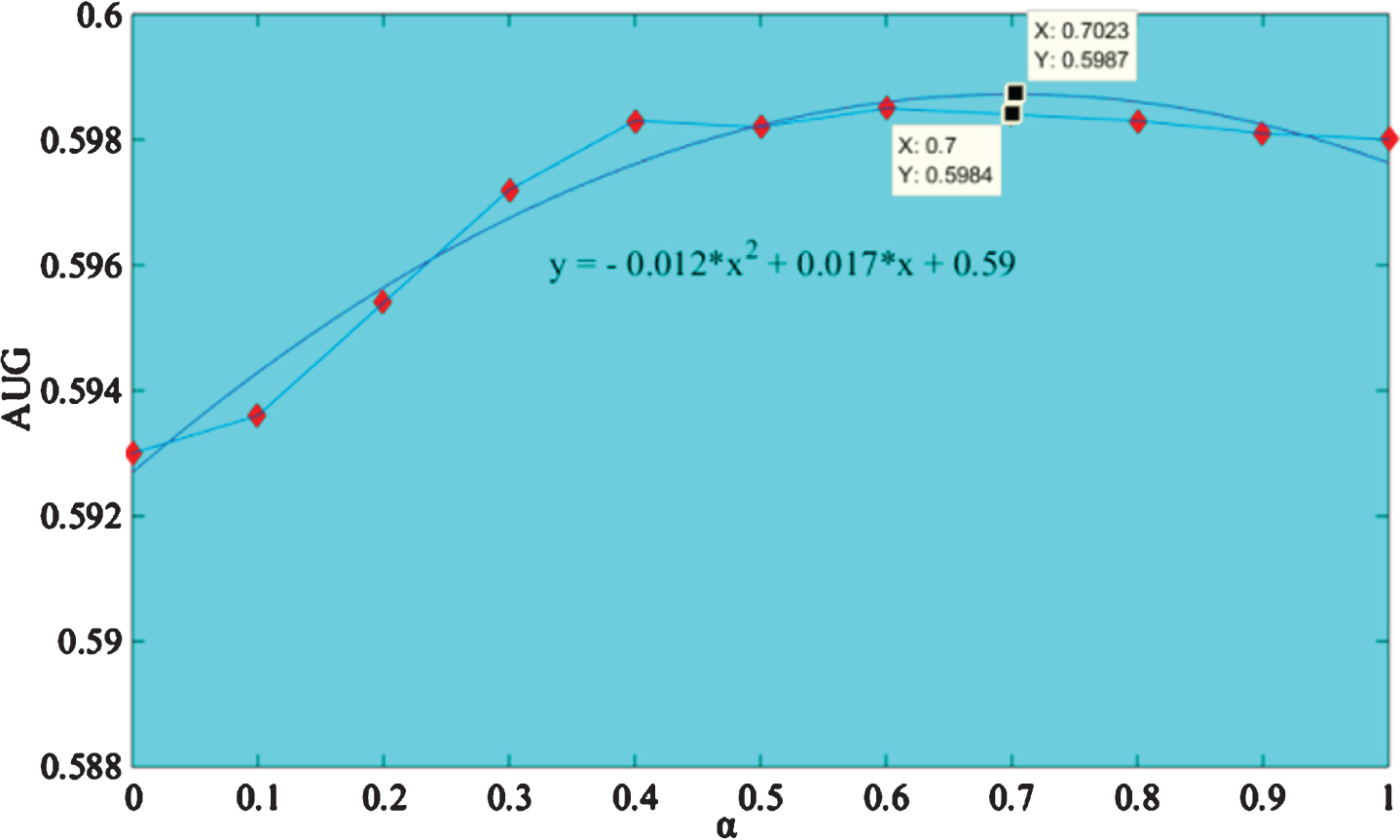
Effect of fusion parameters on model performance.

(3) Analysis of the influence of binary computing types on model effects

How to get the edge vector from the vertex vector is an important problem in the model. To explore the influence of the selection of binary operation types on the model effect, this paper selects Hadamard product, vector average, L1 norm and L2 norm for evaluation. As shown in Fig. 6, in the LINE algorithm, node2vec algorithm, and integration model, the use of Hadamard product as the binary operation between vertices is the most stable, obviously better than the other three operations, and the vector average effect is second. Because geometrically, the vector averaging represents the midpoint between two vertices in the vector space. If the representation of the midpoint is used as the representation of the edge, it may not represent the features of the edge. The L1 norm and L2 norm effects are the worst, and the effects of the two operations are almost the same. When using the norm operation, the obtained value represents the distance between two vertices. If this value is input as a feature value to the classifier, the feature of the edge cannot be fully represented, and the classification effect is poor.

Fig. 6

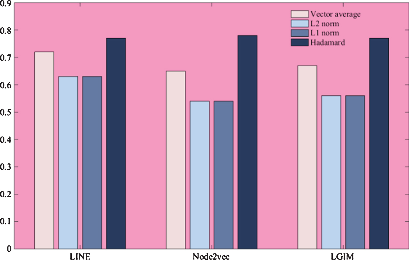
Effect of binary operations on model effects.

(4) Analysis of the influence of model fusion method on model effect

Model fusion technology can generally improve the accuracy of machine learning tasks. Common model fusion methods include weighted averaging, bagging, and boosting. The bagging method performs subsampling in the training set, composes the submarines required for each base model, and votes on the predicted results according to each model. Each model votes with the same weight. The prediction results of all the basic models are combined to produce the final prediction results. The implementation principle of the boosting method is to iteratively train the baseline model. Each time the weight of the training sample is modified according to the prediction error in the previous iteration, the essence is to aggregate multiple decision trees. Each tree is generated sequentially, depending on the previous tree. To explore the influence of the model fusion method on the model effect, this paper selects weighted average, bagging and boosting methods (represented by Adaboost as the representative of the boosting method). Since the classifier selected in the basic experiment is the Logistic Regression Model (LR), to better compare the effect of the fusion model, the weak classification learner in the bagging and boosting methods still uses the LR model, and the rest of the frame parameters are sklearn encapsulation algorithm. The default parameters are shown in Table 2. Figure 7 is obtained from the data in Table 2.

Table 2

Effect of fusion method on model effect

Fusion method	Deep	Deep	node2vec	node2vec
	Walk+LINE	Walk+SDNE	+LINE	+SDNE
Weighted average	0.7796	0.7698	0.7751	0.7765
Bagging	0.7821	0.7711	0.7949	0.7812
Boosting	0.7354	0.7513	0.7201	0.7431

Fig. 7

Effect of fusion method on model effect.

As shown in Fig. 7, the bagging method works best in the three fusion modes, with the weighted average and boosting methods second. Because the boosting method is sensitive to noise data and abnormal data, each time it is iterated, it will give a larger weight to the noise point, so that the latter model pays more attention to the sample that is misclassified, and the over-fitting phenomenon occurs. Over-fitting is very common in machine learning applications. The fundamental problem is that the amount of training data is not enough to support complex models, resulting in the model learning the noise on the data set. The bagging method and the weighted average method can reduce the noise point considerations. To improve the generalization ability of decision boundaries, even the misjudgment of some models will not affect the final result, thus avoiding over-fitting.

4 Conclusions

This paper mainly studies the representation learning problem of node structure features based on large-scale dynamic social networks. By positively and negatively damping the node relationships of different classes, and constructing a local search dynamic sampling algorithm for new network nodes, DNPS model and the latest network feature learning model deep walk and line model are proposed, comparative experiments show that: DNPS model has good feature extraction ability on the large-scale dynamic social network, and its time overhead is effectively controlled. DNPS model is proposed to solve the dynamic problems existing in the distributed feature learning process of large-scale dynamic social networks and the simulation problems of hierarchical relationships in social networks. Finally, we provide the research community with the code and friendliness required for DNPS model training by establishing a project website. The reference document provides a reference for the application of the DNPS model in related fields and the comparison of subsequent algorithms. Network representation learning is one of the emerging research directions in the field of complex networks in the past two years. Learning to get a good representation of network characteristics can not only solve large-scale dynamic social network sparsity and the presence of features such as dynamic problems. Also effectively applied to other child-related fields, such as large-scale dynamic community we found that users classify large-scale social networks and another large-scale diffusion of information on social networking information.

For this paper, for the sake of simplicity, the globally based uniform damping reference values are proposed. Further possible research directions are: (1) Based on the node relationship, construct a dynamic damping model, that is, adopt LSTM (Long Short Term Memory). The “alignment” idea in the model, constructing the “aligned” dynamic damping value for each positive sampling; (2) The super parameters proposed in this paper are slightly redundant, how to further reduce the hyperparameters for different network types. The number reduces the difficulty of the application and improves the training effect of the model.

The research directions beyond the model of this paper may also be: (1) Feature learning of cross-media networks. In the same social network, there are not only structural features between nodes, but also node attributes, community attributes, and edge attributes, a variety of media types, etc. Therefore, how to effectively integrate the characteristics of different media based on the nodes themselves, get more rich network features, it is worth further exploration and analysis; (2) Feature learning of cross-platform networks. In a single network platform, based on effective learning, the characteristics are learned and corresponding to the characteristics of different network platforms. For example, while users have network relationships on Sina Weibo, there may be similar relationships on other social network platforms. So, is it the same user nodes that have the same (or learned) characteristics on different social network platforms? Especially in large-scale environments, this cross-platform consistency correspondence research can effectively mine users. The relationship between them may be one of the effective methods for cross-platform recommendation prediction.

Footnotes

Acknowledgments

This work was supported by (1) the National Natural Science Foundation of China under Grant nos. 61672179, 61370083 and 61402126, (2) the National Natural Science Foundation of Heilongjiang Province of China under Grant no. F2015030, (3) the Youth Science Foundation of Heilongjiang Province of China under Grant no. QC2016083, (4) the Postdoctoral Fund of Heilongjiang Province of China under Grant no. LBH-Z14071.

References

Kamada

, Ichimura

and Harada

, Knowledge extraction of adaptive structural learning of deep belief network for medical examination data, International Journal of semantic computing 13(01) (2019), 67–86.

Jiang

, Zhang

, Duan

, et al., Identify Huntington’s disease-associated genes based on restricted Boltzmann machine with RNA-seq data, BMC bioinformatics 18(1) (2017), 447.

, Chen

and Li

, Hierarchical recurrent neural hashing for image retrieval with hierarchical convolutional features, IEEE Transactions on Image Processing 27(1) (2017), 106–120.

Tian

, Li

, Chen

, et al., Learning subspace-based RBFNN using a coevolutionary algorithm for complex classification tasks, IEEE transactions on neural networks and learning systems 27(1) (2015), 47–61.

Biggs

M.B.

and Papin

J.A.

, Managing uncertainty in metabolic network structure and improving predictions using EnsembleFBA, PLoS computational biology 13(3) (2017), e1005413.

Alnamoly

M.H.

, Alzohairy

A.M.

and El-Henawy

I.M.

, A survey on gel images analysis software tools, Journal of Intelligent Systems and Internet of Things 1(1) (2020), 48–60.

Thomas

E.K.

, Markin

and Oggier

, On Abelian group representability of finite groups, Advances in Mathematics of Communications 8(2) (2017), 139–152.

Thanou

, Dong

, Kressner

, et al., Learning heat diffusion graphs, IEEE Transactions on Signal and Information Processing over Networks 3(3) (2017), 484–499.

Zou

Y.G.

, Lin

W.L.

and Zheng

X.M.

, Spatial-temporal characteristics and influential factors of network attention to tourism security, Tourism Tribune 30(2) (2015), 101–109.

10.

Astvatsatourov

and Mösges

, Specific Characteristics in Digital Assessment of Conjunctival Redness, ICIMTH (2017), 181–184.

11.

Y.H.

, Stangl

, Chipara

, et al., Characteristics of real-world signal-to-noise ratios and speech listening situations of older adults with mild-to-moderate hearing loss, Ear and Hearing 39(2) (2018), 293.

12.

Kim

, Guan

, Waliser

D.E.

, et al., Winter precipitation characteristics in western US related to atmospheric river landfalls: observations and model evaluations, Climate Dynamics 50(1-2) (2018), 231–248.

13.

Yang

, Wu

and Liu

, Bayesian network structure learning based on modified particle swarm optimization, International Journal of Information and Communication Technology 8(1) (2016), 112–121.

14.

Christian

, Boyd

R.N.

and Smarandache

, Three Possible Applications of Neutrosophic Logic in Fundamental and Applied Sciences, International Journal of Neutrosophic Science 1(2) (2020), 90–95.

15.

, Xu

J.M.