Artificial neural networks and adaptive neuro-fuzzy inference systems for parameter identification of dynamic systems

Abstract

There would always be some unknown geometric, inertial or any other kinds of parameters in governing differential equations of dynamic systems. These parameters are needed to be numerically specified in order to make these dynamic equations usable for dynamic and control analysis. In this study, two powerful techniques in the field of Artificial Intelligence (AI), namely Artificial Neural Network (ANN) and Adaptive Neuro-Fuzzy Inference System (ANFIS) are utilized to explain how unknown parameters in differential equations of dynamic systems can be identified. The data required for training and testing the ANN and the ANFIS are obtained by solving the direct problem i.e. solving the dynamic equations with different known parameters and input stimulations. The governing ordinary differential equations of the system is numerically solved and the output values in different time steps are obtained. The output values of the system and their derivatives, the time and the inputs are given to the ANN and the ANFIS as their inputs and the unknown parameters in the dynamic equations are estimated as the outputs. Finally, the performances of the ANN and the ANFIS for identifying parameters of the system are compared based on the test data Percent Root Mean Square Error (% RMSE) values.

Keywords

System identification parameter identification artificial neural network ANFIS

1 Introduction

Artificial Intelligence (AI) is incorporated into a wide variety of researches and technological devices. It also has made its own way into various approaches for identification processes of complex systems. Two of the most powerful AI techniques are Artificial Neural Networks (ANNs) and Adaptive Neuro-fuzzy Inference System (ANFIS).

ANNs have a broad range of applications in solving those problems that the relation between dependent and independent variables is not properly understood [7]. An MLP based decision support system was presented to support the diagnosis of heart diseases. The suggested ANN, had 5 nodes in its output layer, each corresponding to one class of heart disease [24]. Calculation of compressibility factor (z-factor) of natural gases plays an important role in the estimation of their thermodynamic properties. A new model, based on ANNs was presented, trained with experimental data based on Standing and Katz z-factor diagram to predict the z-factor of natural gases [5]. An inverse analysis method is suggested to simulate the A-scan ultrasonic testing, using ANNs and computational mechanics. The ANNs were trained by the characteristic parameters extracted from different surface responses from the direct problem, and then the ANNs were used to classify and identify cracks in the medium [18]. An ANN-based approach for enhancing the accuracy of the electrical equivalent circuit of a photovoltaic module was proposed. The ANN was trained by using some measured current-voltage curves, and the equivalent circuit parameters were approximated by reading the samples of temperature and solar irradiation, without any nonlinear equation being solved, which is needed in conventional methods [14].

ANFIS can be tremendously useful in input-output data relationship modeling [21] and has numerous applications. ANFIS is practical in parameter estimation of PV modules. An ANFIS was modeled to obtain three of the parameters in single-diode model of PV cells namely shunt resistance, series resistance and diode ideality factor by taking short circuit current, material type of PV module, open circuit voltage, and unit area under I-V curve of the PV module as the inputs [16]. Damage identification was done with ANFIS to identify damage in a model steel girder bridge by use of dynamic parameters. The data required were in the form of natural frequencies and were obtained from experimental modal analysis [20]. ANFIS was used for predicting the friction force in CNC linear guideways and servomotor current in the feed drive system in dry lubrication condition. The friction forces were calculated from the cutting force analysis and the servomotor currents were measured during cutting. Finally, an ANFIS was designed to predict these two parameters based on the obtained training data [21].

To study any dynamic system, a mathematical model of that should be driven initially. Most of the time this model contains some parameters that are needed to be estimated for dynamic or control analysis. That’s how parameter identification becomes a very important topic in various fields of science and engineering. Identification of mechanical and electrical parameters of an induction motor has been done with its voltage, current and speed by means of Genetic Algorithm [4]. This job has been done with Differential Evolution approach as well [15]. For non-linear Newton-Euler dynamic equations a transformation is introduced to attain a linear model to identify parameters of a cylindrical robot with such methods like Least Square [23]. ANNs are very applicable tools for parameter identification of dynamic systems apart from their other vast applications. They are used for identification of non-linear switched reluctance machine by measuring its operating data [19]. They are also utilized to identify parameters of Gurson–Tvergaard–Needleman model that is used for predicting mechanical ductile damage [1]. ANNs are applied to identify parameters of a theoretical model for predicting behavior of a fibrous composite under a specific cycling loading [17]. Like ANNs, ANFIS is the other AI tool that is immensely valuable for parameter identification as well. ANFIS is applied to estimate the state of charge parameter of a specific kind of battery [6]. They are utilized for online identification of induction motors [3]. They also are used for identification of the Young’s modulus of rocks [22].

These are just examples from a large body of research have been done on ANN and ANFIS applications in different areas, identification via traditional and artificial intelligence approaches. As a matter of fact, to date research lacks the use of ANN and ANFIS and their comparison with each other for estimating the unknown parameters that exist in dynamic differential equations of systems. Thus, the main contribution of this research is to use these two AI tools so as to identify the above mentioned parameters and to compare these two techniques for solving such problems.

The rest of the paper is organized as follows: Section 2 summarizes the preliminaries which contains some basic information about ANNs and ANFIS structure and their mathematical formulation. In Section 3 the methodology used in this research is explained with an example. Section 4 demonstrates how to generate the data for training both the ANNs and the ANFISs. Section 5 is dedicated to identify the parameters with ANN technique. After that in Section 6 the identification procedure is done with ANFIS technique. Section 7 is going to discuss the results and compare the ANN and ANFIS performance with each other. Eventually, the conclusions are demonstrated in Section 8.

2 Preliminaries

2.1 Artificial neural networks (ANN)

ANNs are very powerful tools in the field of AI. Researchers got interested in this field since the beginning of the 1980s. They are widely used in pattern classification, clustering, function approximation, prediction, control and many other fields [10]. ANNs are inspired mainly by biological neural networks in the human brain. A biological neuron comprises a cell body, and two tree-like branches called the axon and the dendrites. A signal enters a neuron through its dendrites, and afterwards the cell body does a simple process on it, and then a signal will exit from the cell via its axon to other neurons [10]. ANNs are a huge number of parallel computing units consisting of a great number of simple processors with so many connections among themselves [10].

Figure 1 shows a neuron model. As can be seen, x₁, x₂, …, x_m are the inputs to the neuron and they are each multiplied to synaptic weights of w_k1, w_k2, … , w_km, respectively. They are then summed with a bias, b_k in an adder element, subsequently, the result is entered to an activation function. Finally, the output value will be exited from the activation function.

Fig. 1

Model of a neuron [8].

In a mathematical point of view, the neuron represented in Fig. 1 can be modeled with Equations (1) and (2) [8], $u_{k} = \sum_{j = 1}^{m} w_{kj} x_{j}$ (1) $y_{k} = φ (u_{k} + b_{k})$ (2)

The activation function φ (.) can be a threshold function, a piecewise linear, sigmoid, Gaussian, or other similar functions [10]. In this research ‘tansig’ function of Matlab software is used whose definition is shown in Equation (3) [25]. $tansig (n) = \frac{2}{(1 + exp (- 2 * n))} - 1$ (3)

There are different sorts of ANNs. The most common form of feed-forward networks is Multilayer Perceptrons (MLPs). In this type of networks, neurons are organized in several layers and there is a unidirectional connection between them [10].

The weights and biases in ANNs are adjustable parameters that an optimization algorithm is needed to update them in such a way that the ANN, favorably performs the task required. There are different training algorithms available and Levenberg-Marquardt was the one trained the ANNs in this research.

2.2 Adaptive Neuro-Fuzzy Inference System (ANFIS)

Adaptive Neuro-Fuzzy Inference System (ANFIS) is a feedforward adaptive neural network whose construction is based on a fuzzy inference system [2]. Jang was among the first to introduce ANFIS [12]. In ANFIS structure, Sugeno-type fuzzy system is merged with neural learning ability. The goal in ANFIS is to optimize the parameters of the fuzzy system, using input-output data samples with a learning algorithm. This task is carried out in such a way that the error between the ANFIS outputs and the target outputs be minimized [9, 13].

In order to explain the ANFIS architecture, a Fuzzy Inference System (FIS) is assumed that has two inputs x and y, and output z. It is supposed that the rule base consists of two fuzzy rules of sugeno-type (4).

$\begin{matrix} Rule 1 : If x is A_{1} and y is B_{1}, then f_{1} = p_{1} x + q_{1} y + r_{1}, \\ Rule 2 : If x is A_{2} and y is B_{2}, then f_{2} = p_{2} x + q_{2} y + r_{2} . \end{matrix}$ (4)

Figure 2 depicts the ANFIS structure which basically consists of five layers [9]. The function of each layer will be explained.

Fig. 2

Model of an ANFIS [12].

Layer 1: This layer is a fuzzifier and A_i and B_i are the linguistic variables. O_i specifies the membership function of A_i and it represents the degree to which the input x belongs to A_i (5). $O_{i} = μ_{A_{i}} (x)$ (5)

Layer 2: Each node in this layer multiplies the incoming signals and sends the result out as in Equation (6). $w_{i} = μ_{A_{i}} (x) \times μ_{B_{i}} (y), i = 1, 2 .$ (6)

Layer 3: This layer does the task of normalization and normalizes the w₁ and w₂ weights with Equation (7). ${\bar{w}}_{i} = \frac{w_{i}}{w_{1} + w_{2}}, i = 1, 2 .$ (7)

Layer 4: This layer computes the contribution of the i’th rule toward the overall output with Equation (8). $\bar{w_{i}} . \bar{f_{i}} = \bar{w_{i}} . (p_{i} x + q_{i} y + r_{i})$ (8)

Layer 5: This layers computes the final output by adding all the incoming signals from layer 4 as shown in Equation (9). $f = \sum_{i} \bar{w_{i}} . f_{i} = \frac{\sum_{i} w_{i} . f_{i}}{\sum_{i} w_{i}}$ (9)

There are a number of methods for creating the initial FIS. Grid Partitioning, Subtractive Clustering and Fuzzy c-Means (FCM) are the most common ones. FCM is the method used in this research to create the initial FISs.

In ANFIS training, there are two types of parameters that are needed to be optimized. The first is belonging to the parameters of the membership functions and the second is the parameters {p_i, q_i, r_i} in Equation (4). There are different methods for doing this optimization. Derivative-based algorithms like gradient descent and heuristic algorithms like genetic algorithm [9]. In this research hybrid method is used which is a combination of least-square estimation and back-propagation [2].

3 Methodology

This section is going to explain the method developed in this research by an example of a two-axis gimbal system. After this approach is illustrated, other systems can also be identified by the same method as well.

In the first place, it is essential to have the dynamic equations of a two-axis gimbal. These equations are available in the literature [11]. The dynamic equations governing the azimuth and elevation axes are expressed in Equations (10) and (11), respectively.

$\begin{matrix} ((I_{1_{22}} + I_{2_{33}}) + (I_{2_{11}} - I_{2_{33}}) \sin^{2} (q_{2})) \overset{. .}{q_{1}} \\ + (I_{2_{11}} - I_{2_{33}}) sin (2 q_{2}) \dot{q_{1}} \dot{q_{2}} + F_{s} sgn (\dot{q_{1}}) = τ_{1} \end{matrix}$ (10)

$\begin{matrix} I_{2_{22}} \overset{. .}{q_{2}} - \frac{1}{2} (I_{2_{11}} - I_{2_{33}}) sin (2 q_{2}) {\dot{q_{1}}}^{2} \\ + k sin (q_{2}) + F_{s} sgn (\dot{q_{2}}) = τ_{2} \end{matrix}$ (11)

Where q₁ is the azimuth angle and q₂ is the elevation angle of the gimbal. I_{i
_jk} is the component of the j’th row and k’th column of the i’th axis’ matrix of moment of inertia which is completely illustrated in [11] and τ₁ and τ₂ are the torques exerted to the azimuth and elevation axis, respectively.

Equations (10) and (11) won’t be fully defined until the values of their inertial and frictional terms be specified, but it is clear that the response of the system does not depend on the values of I_1₂₂, I_2₃₃ and, I_2₁₁ independently. The values of (I_1₂₂ + I_2₃₃) and (I_2₁₁ - I_2₃₃) besides I_2₂₂, k and F_s are the values that determine the response of the system independently [11]. In this case, Equations (10) and (11) will change into Equations (12) and (13).

$\begin{matrix} (A_{1} + A_{2} {sin}^{2} (q_{2})) {\ddot{q}}_{1} + A_{2} sin (2 q_{2}) {\dot{q}}_{1} {\dot{q}}_{2} \\ + F_{s} sgn ({\dot{q}}_{1}) = τ_{1} \end{matrix}$ (12)

$\begin{matrix} A_{3} {\overset{. .}{q}}_{2} - \frac{1}{2} A_{2} sin (2 q_{2}) {\dot{q}}_{1}^{2} + A_{4} sin (q_{2}) \\ + F_{s} sgn ({\dot{q}}_{2}) = τ_{2} \end{matrix}$ (13)

In these equations, parameters A₁, A₂, A₃ and A₄ are defined as Equation (14) [11].

$\begin{matrix} A_{1} = (I_{1_{22}} + I_{2_{33}}), A_{2} = (I_{2_{11}} - I_{2_{33}}), \\ A_{3} = I_{2_{22}}, A_{4} = k \end{matrix}$ (14)

Equations (12) and (13) are the main equations in this research and the parameters that are going to be identified are A₁, A₂, A₃, A₄, and F_s.

As mentioned earlier, the ANN and the ANFIS need data to be trained. Those data should satisfy Equations (12) and (13).

There are two common approaches to acquire these data. The first one, which is the one, going to be implemented in this research, is to assign some arbitrary values to A₁, A₂, A₃, A₄, and F_s and to set arbitrary values for τ₁ and τ₂, as well. After this, solve each pair of equations produced with a numerical method. By doing so q₁, q₂ and their derivatives will be available. The second way is to prepare several 2-axis gimbals, exert known torques τ₁ and τ₂ to each of their axes, subsequently measure the q₁, and q₂ angles with optical encoders in different time steps and following this, calculate q₁ and q₂ derivatives with numerical methods.

Finally, the inverse problem will be solved with τ₁ and τ₂, q₁ and q₂, and their first and second derivatives considered as the inputs to the ANN and the ANFIS, and gimbal parameters namely A₁, A₂, A₃, A₄, and F_s considered as the outputs.

4 Generating the training data

The first step to generate the data required to train the ANN and the ANFIS is to assign some values to A₁, A₂, A₃, A₄, and F_s. Also a number should be given for each τ₁ and τ₂. Parameters of A₁, A₂, A₃, and A₄ are assigned to 1, 1.3, 1.6, and 1.9. F_s is given 0.1, 0.2, 0.3, 0.4 values and each τ₁ and τ₂ are assigned to 3. Consequently, there will be 4 values for each A₁, A₂, A₃, A_4, and F_s and 1 value for each τ₁ and τ₂, therefore by considering the rule of product, 4*4*4*4*1*1 = 1024 combinations will be available resulting in 1024 different equations to be solved.

These equations are solved with ode45 function in Matlab with zero initial conditions for a time interval of 0 to 3 second and a 0.001 s time step.

After solving each of the 1024 equations produced, the answers for each one will be $q_{1}, {\dot{q}}_{1}, q_{2}$ , and ${\dot{q}}_{2}$ values in 0 to 3 seconds interval in each 0.001 s time steps. In other words, a dataset with 3001 elements will be available after solving each equation. As a result, there will be 1024*3001 = 3,073,024 different data samples after solving all the 1024 equations.

This dataset doesn’t include the second derivatives of the q₁ and q₂. Therefore, a numerical derivation can be used to calculate for $\overset{. .}{q_{1}}$ and $\overset{. .}{q_{2}}$ . The amount of 3,073,024 data samples is too large to be dealt with in training an ANN or an ANFIS, especially an ANFIS. In this research, it was experienced that the ANFIS toolbox and the FCM option in Matlab is too time-consuming for datasets containing more than 10,000 data samples. To tackle this problem 10,000 data samples were randomly picked from these 3,073,024 data records and stored as the dataset for training and testing the ANN and ANFIS.

The accuracy of each elements of this dataset were tested by substituting q₁ and q₂ and their derivatives into Equations (12) and (13) to calculate for τ₁ and τ₂. After that, the errors between these computed values and the initially assigned values for τ₁ and τ₂. (i.e. ‘3’) were calculated. The % error and the % RMSE are calculated with Equations (15) and (16), respectively and are depicted in Fig. 3. $% error = \frac{T - \bar{T}}{T} * 100$ (15)

$% R M S E = 100 \sqrt{\frac{1}{n} \sum^{} {(\frac{T - \bar{T}}{T})}^{2}^{}}$ (16)

T: initially assigned value $\bar{T}$ : computed value

It can be seen that the computed data % RMSE is 4.28% and 2.26% for τ₁ and τ₂, respectively. Hence the calculated data is sufficiently accurate.

Fig. 3

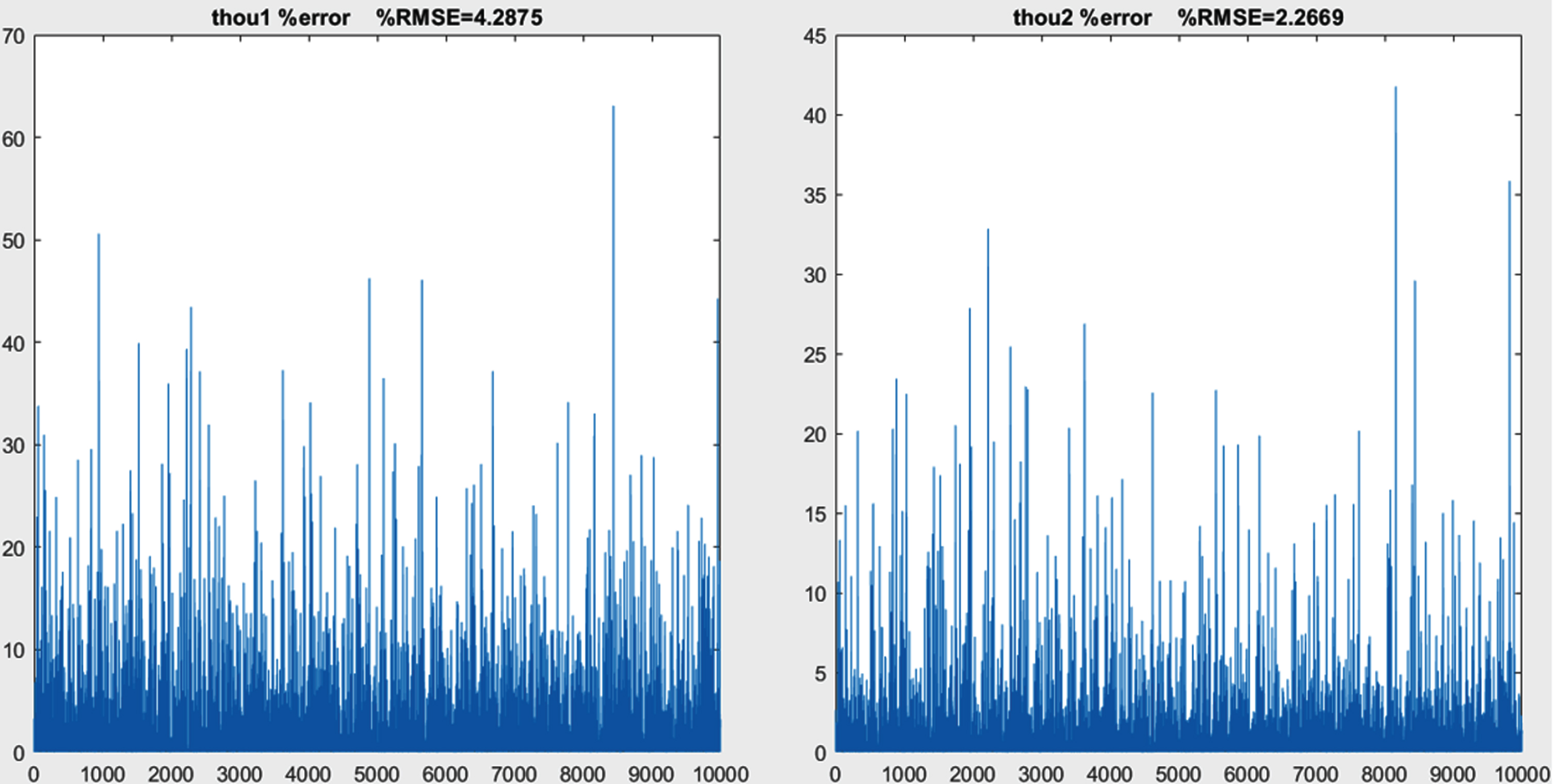
% Error chart corresponding to the accuracy of calculated dataset.

5 Parameter identification with the ANN

In the first place, it should be decided what parameters should be the inputs and outputs of the ANN. To find which parameters should be assigned as inputs, four different models are assumed. Model 1 is an ANN which takes just τ₁ and τ₂, q₁, and q₂ as its inputs. Model 2 is an ANN which takes τ₁ and τ₂, q₁, q₂, and t (time) as its inputs. Next model, model 3, takes τ₁ and τ₂, q₁, q₂, ${\dot{q}}_{1}$ , ${\dot{q}}_{2}$ , and t as the inputs and finally, model 4 takes τ₁ and τ₂, q₁, q₂, ${\dot{q}}_{1}$ , ${\dot{q}}_{2}$ , ${\ddot{q}}_{1}$ , ${\ddot{q}}_{2}$ , and t as its inputs. The output from each ANN is one of the A₁, A₂, A₃, A₄ and F_s. The appropriate ANN hidden layer size might be different for estimating each of the A₁, A₂, A₃, A_4, and F_s. The reason why it is considered one output for each ANN is to make ourselves able to adjust the hidden layer size for estimating each parameter separately. Each of these four models is going to be tested to find out which one is the best.

The neural network toolbox of Matlab software is used to solve the problem by ANN technique, in this research. 70% of the 1000 data samples are randomly selected as the training data, and a pair of 15% of data samples are selected as testing and validating data. The training algorithm is Levenberg-Marquardt with 1000 iterations, and the objective function is mse. There is just one hidden layer for each ANN, and 3 ANNs with 10, 20 and 30 neurons are trained separately for each parameter. After training each ANN, the Test Data % RMSE of each of them are calculated with Equation (17). All the resulted values are depicted in Fig. 4. Table 1 is to find out which model, parameter, and hidden layer size is belonging to each run number. $% RMSE = 100 \sqrt{\frac{1}{n} \sum {(\frac{z - \bar{z}}{z})}^{2}}$ (17) $Z = Targets value \bar{Z} = Output value$

Fig. 4

Test Data % RMSE comparison for all models in each run number.

Table 1

Description of each run number

Run Number	1	2	3	4	5	6	7	8
Parameter	A₁	A₁	A₁	A₂	A₂	A₂	A₃	A₃
Hidden layer size	10	20	30	10	20	30	10	20
Run Number	9	10	11	12	13	14	15
Parameter	A₃	A₄	A₄	A₄	F_s	F_s	F_s
Hidden layer size	30	10	20	30	10	20	30

It can be inferred from Fig. 4 that the Test Data % RMSE for model 2 is less than that of model 1, and Test Data % RMSE for model 3 is better than that of model 2, and finally model 4 has the least amount of Test Data % RMSE in each run number.

It can be concluded from Fig. 4 that the % RMSE of the run numbers 1, 2, and 3 which belong to the parameter A₁ and 7, 8, and 9 which belong to the parameter A₃ are 3.95% and 4.26%, respectively, each with 30 neurons in one hidden layer, and this result is promising. But the errors for the run numbers 4, 5, and 6 which correspond to the parameter A₂, 10, 11, and 12 which belong to the parameter A4 and 13, 14, and 15 which belong to the parameter F_s are a little higher and thus less acceptable, hence it sounds like a good idea to train more complicated ANNs for parameters A₂, A₄, and F_s to improve the accuracy. Using more complicated ANNs in here, means considering more hidden layers.

For the parameter A₂, different hidden layer sizes, as in Table 2, are considered. % RMSE for each run number is calculated with Equation (17), and they are all depicted in Fig. 5. It is seen that the run number 11 with 6 8 8 8 8 6 hidden layer size is the best ANN with 6.45% Test Data % RMSE.

Table 2

Description of each run number for A₂

Run Number	1	2	3	4
Hidden Layer size	10 10	20 20	30 30	7 7 7
Run Number	5	6	7	8
Hidden Layer size	7 10 7	5 10 5	6 8 10 8 6	8 8 10 8 6
Run Number	9	10	11
Hidden Layer size	8 10 10 8 6	6 8 8 10 8 6	6 8 8 8 8 6

Fig. 5

% RMSE for parameter A₂ in every run number.

This task is also done for the parameter A₄. Different hidden layer sizes, as in Table 3, are considered and % RMSE for each run number is depicted in Fig. 6. It is seen that the run number 3 with 30 30 hidden layer size is the best ANN with 6.18% Test Data % RMSE.

Table 3

Description of each run number for A₄

Run Number	1	2	3	4	5
Hidden Layer size	10 10	20 20	30 30	10 20 10	10 10 10
Run Number	6	7	8	9
Hidden Layer size	8 10 8	4 6 6	10 10 10 10	10 12 12 10

Fig. 6

% RMSE for parameter A4 in every run number.

Also for the parameter F_s, various hidden layer sizes, as in Table 4, are considered. % RMSE for each one is depicted in Fig. 7. It is seen that the run number 10 with 10 12 14 12 10 hidden layer size is the best ANN with 19.57% Test Data % RMSE.

Table 4

Description of each run number for F_s

Run Number	1	2	3	4
Hidden Layer size	20 20	30 30	10 10 10	10 20 15
Run Number	5	6	7	8
Hidden Layer size	10 18 10	13 13 13	14 14 14	15 15 15 15
Run Number	9	10	11	10
Hidden Layer size	14 16 18 16 14	10 12 14 12 10	16 16 16	15 16 16

Fig. 7

% RMSE for parameter F_s in every run number.

As a final result, the best ANNs trained for each parameter are written in Table 5.

Table 5

Accuracy of the best ANN trained for identification of each parameter

Parameter	Best Hidden Layer Size	Train Data % RMSE	Test Data % RMSE	All Data % RMSE
A₁	30	3.70	3.95	3.77
A₂	6 8 8 8 8 6	6.01	6.45	6.08
A₃	30	3.79	4.26	3.88
A₄	30 30	6.11	6.18	6.26
F_s	10 12 14 12 10	10.50	19.57	16.58

As can be seen all the results for all the parameters are promising. The parameter F_s seems to have more error than the other parameters. This shows that this method might not be the best option for identification of the parameter F_s.

6 Parameter identification with the ANFIS

In the previous section it was concluded that for solving this problem, τ₁,τ₂, q₁, q₂, ${\dot{q}}_{1}$ , ${\dot{q}}_{2}$ , ${\ddot{q}}_{1}$ , ${\ddot{q}}_{2}$ , and t are the best inputs for ANNs. It seems very logical to take these parameters as the inputs to solve the problem with ANFIS as well. Like in training ANNs, for each ANFIS one of the parameters A₁, A₂, A₃, A₄, F_s is considered as the output.

Each one of the ANFIS modeled in this research are implemented in Matlab with 70% of the data samples divided as Train Data and the rest 30% as the Test Data. Hybrid method which is a combination of back-propagation and least-square estimation is used to train each ANFIS. Fuzzy c-means (FCM) is adopted to create the initial FIS. A number of 10, 20, 30, 40, 50 and more clusters are tested in order to find out what the best number of clusters is for identifying each parameter.

To find out how many clusters is the best for creating the initial FIS for identification of parameter A₁, different ANFISs with different initial FISs are trained in 300 epochs. Differences in initial FISs are the number of their clusters in FCM options. After training each ANFIS, the values of % RMSEs are calculated with Equation (17) for different data types and the values are shown in Table 6.

Table 6
% RMSE in ANFIS, with different numbers of clusters in initial FIS, for A₁ identification

Number of Clusters Train Data % RMSE Test Data % RMSE All Data % RMSE

10 14.79 14.46 14.69

20 12.68 12.59 12.66

30 10.59 10.87 10.92

40 10.08 10.12 10.09

50 11.98 11.91 11.95

Number of Clusters	Train Data % RMSE	Test Data % RMSE	All Data % RMSE
10	14.79	14.46	14.69
20	12.68	12.59	12.66
30	10.59	10.87	10.92
40	10.08	10.12	10.09
50	11.98	11.91	11.95

Based on the Test Data % RMSE, the best number of clusters for identification of parameter A₁ is 40. Training of the ANFIS that was created with 40 clusters is continued to 6000 epochs. Test Data % RMSE for different epochs are shown in Fig. 8. Epoch 6000 is where the ANFIS has the least amount of error in Test Data, i.e. 6.81%.

Fig. 8

ANFIS Test Data % RMSE in different epochs for parameter A₁ identification.

This same procedure is done for parameter A₂ and the % RMSE for different data types are shown in Table 7.

Table 7

% RMSE in ANFIS, with different numbers of clusters in initial FIS, for A₂ identification

Number of Clusters	Train Data % RMSE	Test Data % RMSE	All Data % RMSE
10	22.69	22.59	22.93
20	23.19	23.48	23.28
30	22.69	22.59	22.93
40	22.80	23.12	22.90
50	23.01	23.34	23.11

Based on Test Data % RMSE in Table 7, the best number of clusters is 30 for identification of the parameter A2. Training procedure for the ANFIS with this number of clusters is continued. Test Data % RMSE is shown in Fig. 9 and epoch 10000 contains the best result, i.e. 18.47%.

Fig. 9

ANFIS Test Data % RMSE in different epochs for parameter A₂ identification.

This procedure is done for parameter A₃, as well and the % RMSE for different data types are shown in Table 8.

Table 8

% RMSE in ANFIS, with different numbers of clusters in initial FIS, for A₃ identification

Number of Clusters	Train Data % RMSE	Test Data % RMSE	All Data % RMSE
10	11.92	12.32	12.04
20	10.73	11.05	10.83
30	10.03	10.56	10.19
40	9.20	9.47	9.28
50	9.07	9.54	9.21
60	9.02	9.87	9.28
70	8.56	9.21	8.82

Based on Table 8, the best number of clusters is 70 for identification of the parameter A₃. Training procedure for the ANFIS with this number of clusters is continued. Test Data % RMSE is shown in Fig. 10 and epoch 10000 represents the least amount of error, i.e. 5.97%.

Fig. 10

ANFIS Test Data % RMSE in different epochs for parameter A₃ identification.

This procedure is done for parameter A₄, too and the % RMSE for different data types are shown in Table 9.

Table 9

% RMSE in ANFIS, with different numbers of clusters in initial FIS, for A₄ identification

Number of Clusters	Train Data % RMSE	Test Data % RMSE	All Data % RMSE
10	23.99	24.16	24.04
20	23.90	24.13	23.97
30	23.05	23.26	23.12
40	22.82	23.11	22.91
50	23.26	23.58	23.35
60	23.72	23.08	23.83
70	22.26	22.75	22.41
80	23.38	23.79	23.51

Based on Table 9, the best number of clusters is 70 for identification of the parameter A₄. Training procedure for the ANFIS with this number of clusters is continued. Test Data % RMSE is shown in Fig. 11 and epoch 5000 represents the least error, i.e. 20.00%.

Fig. 11

ANFIS Test Data % RMSE in different epochs for parameter A₄ identification.

The procedure is done for parameter F_s, too and the % RMSE for different data types are shown in Table 10.

Table 10

% RMSE in ANFIS, with different number of cluster in initial FIS, for F_s identification

Number of Clusters	Train Data % RMSE	Test Data % RMSE	All Data % RMSE
10	72.88	73.38	73.03
20	72.83	73.40	73.00
30	73.10	74.23	73.44
40	76.65	77.26	76.83
50	73.07	74.88	73.61
60	71.34	73.09	71.87
70	75.01	76.44	75.44
80	71.68	73.56	72.25

Based on Table 10, the best number of clusters is 60 for identification of the parameter F_s. Training procedure for the ANFIS with this number of clusters was continued. Test Data % RMSE is shown in Fig. 12 and epoch 300 represents the least error i.e. 73.09%.

Fig. 12

ANFIS Test Data % RMSE in different epochs for parameter F_s identification.

As a summary, the best ANFIS designed for each parameter is shown in Table 11.

Table 11

Accuracy of the best ANFIS trained for identification of each parameter

parameter	Number of clusters	All Data % RMSE	Test Data % RMSE	Train Data % RMSE
A₁	40	6.56	6.81	6.63
A₂	30	17.93	18.47	18.09
A₃	70	5.33	5.97	5.53
A₄	70	19.76	20.00	19.84
F_s	60	71.34	73.09	71.87

It is seen from Table 11, that the parameters A₁ and A₃ are identified successfully with this method and the amount of errors for parameters A₂ and A₄ are to some extent good but the % RMSE for parameter F_s is unacceptable in spite of considerable efforts in trying different ANFISs with several initial FISs with different numbers of clusters.

7 Discussion of the results

In this section, the performance of ANN and ANFIS for each parameter is discussed. Table 12 shows the best Test Data % RMSE for different parameters, identified with both ANN and ANFIS techniques. Also these values can be compared in Fig. 13.

Table 12
Test Data % RMSE of the best ANN and ANFIS trained for each parameter

parameter ANFIS Test Data % RMSE ANN Test Data % RMSE

A₁ 6.81 3.95

A₂ 18.5 6.45

A₃ 5.97 4.26

A₄ 20 6.18

F_s 73.1 19.57

parameter	ANFIS Test Data % RMSE	ANN Test Data % RMSE
A₁	6.81	3.95
A₂	18.5	6.45
A₃	5.97	4.26
A₄	20	6.18
F_s	73.1	19.57

Fig. 13

Comparison of the performance of ANN and ANFIS for identification of each parameter.

As can be seen ANN resulted in a better accuracy rather than ANFIS in estimating all of the parameters A₁, A₂, A₃, A₄, and F_s. In fact Test Data % RMSE for ANFIS is 2 - 3 times of that for ANN.

All of the parameters identified successfully with ANN. Although Test Data % RMSE for identifying F_s is a little more compared to other parameters, it is still much more acceptable than how ANFIS performed.

Better performance of the ANNs is basically because of possessing multiple layers of neurons. In fact, if a specific size of hidden layer doesn’t result in a good accuracy, increasing the number of neurons and increasing the number of hidden layers, in most cases will cause in a better accuracy, although in this process, care should be taken to avoid overtraining. On the other hand, when it comes to ANFIS training, if the ANFIS doesn’t result in a good accuracy, changing the initial FIS can improve the performance but as what was seen in this research, this work has a minor effect on improving the performance.

One of the main reasons why ANFIS performed worse than ANN in this research, is because ANFIS has a lot more parameters in itself to be optimized in training process. Take the identification has been done for parameter F_s in this research for example. This estimation was done by ANFIS with an initial FIS with 60 clusters. The resulted ANFIS had 1680 parameters in itself to be optimized. This job was done with ANN as well with 10 12 14 12 10 hidden layer size, which was almost the most complicated ANN trained in this research, and it only created 715 parameters in itself to be optimized, which is less than half of the number of adjustable parameters in the ANFIS. This fact shows that identifying these parameters are much more challenging for ANFIS, although ANFIS performed fairly well for identification of all the parameters except for F_s.

The other reason for lack of performance in ANN and ANFIS could be the possible errors in train and test data. As shown in Fig. 3, there are a little amount of error in the generated data. Although ANN and ANFIS are very strong tools that are capable of handling such noises and errors, they are expected to perform better with more accurate datasets that follow the dynamic equations of the system precisely.

8 Conclusions

In this research, identification of unknown parameters in dynamic equations of systems was studied with ANN and ANFIS techniques. It was seen that both these tools are very powerful for identification of the parameters in dynamic equations of systems. Although ANFIS performed fairly well in identification of all parameters except the friction factor, it was concluded that ANN is stronger for doing this task in comparison with ANFIS. In fact the values of % RMSE of the ANN results were 2-3 times lower than those of the ANFISs. ANNs trained in this study had less number of adjustable parameters to be optimized in comparison with ANFIS, and probably this is the reason why ANN performed better.

In this study it was assumed that there is no other noise on the data except the error that was created in the phase of generating data with ode45 function, which was shown in Fig. 3. Implementing this method by generating the data with experimental work and imposing some noise on the data and comparing the results would be subjects for further research.

References

Abbassi

, Belhadj

, Mistou

and Zghal

, Parameter identification of a mechanical ductile damage using Artificial Neural Networks in sheet metal forming, Materials & Design 45 (2013), 605–615.

Alavandar

and Nigam

M.J.

, Inverse Kinematics Solution of 3DOF Planar Robot using ANFIS International Journal of Computers, Communications & Control 3(3) (2008), 150–155.

Ali

M.M.I.

and Hassan

M.A.M.

, Parameter Identification Using ANFIS for Magnetically Saturated Induction Motor, International Journal of System Dynamics Applications 1(2) (2012), 28–43.

Alonge

, Raimondi

, Ferrante

and Dippolito

, Parameter identification of induction motor model using genetic algorithms, IEE Proceedings - Control Theory and Applications 145(6) (1998), 587–593.

Azizi

, Rezakazemi

and Zarei

M.M.

, An intelligent approach to predict gas compressibility factor using neural network model, Neural Computing and Applications 31(1) (2019), 55–64.

Cai

, Du

and Liu

, Battery state-of-charge (SOC) estimation using adaptive neuro-fuzzy inference system (ANFIS), The 12th IEEE InternationalConference on Fuzzy Systems, 2003.

Garcia

L.A.

and Shigidi

, Using neural networks for parameter estimation in ground water, Journal of Hydrology 318(1–4) (2006), 215–231.

Haykin

, Neural Networks and Learning Machines, Hamilton, Ontario, Canada: Pearson, 2009.

Haznedar

and Kalinli

, Training ANFIS Using Genetic Algorithm for Dynamic Systems Identification, IJISAE (2016), 44–47.

10.

Jain

A.K.

, Mao

and Mohiuddin

K.M.

, Artificial neural networks: a tutorial, Computer 29(3) (1996), 31–44.

11.

Jahanandish

, Khosravifard

, Vatankhah

and Cheraghi

, Parameter Estimation and Fuzzy Controller Design for a Two-Axis Gimbal, Intelligent and Fuzzy Techniques in Big Data Analytics and Decision Making Advances in Intelligent Systems and Computing (2019), 89–97.

12.

Jang

J.-S.R.

, ANFIS: Adaptive-Network-Based Fuzzy Inference System, IEEE Transactions On Systems, Man, and Cybernetics 23(3) (1993), 150–155.

13.

Jang

J.y.-S.h.R.

, Input Selection for ANFIS Learning, in Proceedings of IEEE 5th International Fuzzy Systems, New Orleans, LA, USA 2 (1996), 1493–1499.

14.

Karatepe

, Boztepe

and Colak

, Neural network based solar cell model, Energy Conversion and Management 47(9–10) (2006), 1159–1178.

15.

Khosla

and Kanade

, Parameter identification of robot dynamics, 1985 24th IEEE Conference on Decision and Control, 1985.

16.

Kulaksız

, ANFIS-based parameter estimation of one-diode equivalent circuit model of PV modules, in 12th IEEE International Symposium on Computational Intelligence and Informatics, Budapest, Hungary, equivalent circuit model of PV modules, 2011.

17.

Lefik

and Schrefler

, Artificial neural network for parameter identifications for an elasto-plastic model of superconducting cable under cyclic loading, Computers & Structures 80(22) (2002), 1699–1713.

18.

Liu

S.W.

, Huang

J.H.

, Sung

J.C.

and Lee

C.C.

, Detection of cracks using neural networks and computational mechanics, Computer Methods in Applied Mechanics and Engineering 191(25–26) (2002), 2831–2845.

19.

, Keyhani

and Fardoun

, Neural network-based modeling and parameter identification of switched reluctance motors, IEEE Transactions on Energy Conversion 18(2) (2003), 284–290.

20.

Razak

S.H.a.H.A.

, Adaptive Neuro Fuzzy Inference System (ANFIS) and Artificial Neural Networks (ANNs) for structural damage identification, Structural Engineering and Mechanics 45(6) (2013), 779–802.

21.

Sparham

, Sarhan

A.A.D.

, Mardi

N.A.

, Hamdi

and Dahari

, ANFIS modeling to predict the friction forces in CNC guideways and servomotor currents in the feed drive system to be employed in lubrication control system, Journal of Manufacturing Processes 28(1) (2017), 168–185.

22.

Singh

, Kainthola

and Singh

, Estimation of elastic constant of rocks using an ANFIS approach, Applied Soft Computing 12(1) (2012), 40–45.

23.

Ursem

and Vadstrup

, Parameter identification of induction motors using differential evolution, The 2003 Congress on Evolutionary Computation, 2003.

24.

Yan

, Jiang

, Zheng

, Peng

and Li

, A multilayer perceptron-based medical decision support system for heart disease diagnosis, Expert Systems with Applications 30(2) (2006), 272–281.

25.

“tansig,” MathWorks, [Online]. Available: https://www.mathworks.com/help/deeplearning/ref/tansig.html.