Cantor set based neighbor generation method for permutation solution representation

Abstract

Metaheuristics gained world-wide popularity and researchers have been studying them vigorously in the last two decades. A relatively less explored approach in the improvement of metaheuristics is to design new neighbor generation mechanisms. Neighbor generation mechanisms are very important in the success of any single solution-based heuristic since they directly guide the search. In this study, a neighbor generation mechanism called cantor-set based (CB) method for single solution-based heuristics which use permutation solution representation is described. The inspiration for CB method stems from the recursive algorithm that constructs a cantor set which is a fractal set. Three variations of CB method are discussed (CB-1, CB-2, CB-3) considering the presented design possibilities. The computational experiments are conducted by embedding the mechanisms into the classical local search and simulated annealing algorithms, separately, to test their efficiency and effectiveness by comparing them to classical swap and insertion mechanisms. The traveling salesman problem (TSP) and quadratic assignment problem (QAP) which are very different problems that have incompatible characteristics have been chosen to test the mechanisms and sets of benchmark instances with varying sizes are chosen for the comparisons. The computational tests show that CB-2 gives very favorable results for TSP and CB-1 gives favorable results for QAP which means that CB-2 is suitable for problems that have steep landscapes and CB-1 is suitable for the problems that have flat landscapes. It is observed that CB-3 is a more generalized mechanism because it gives consistently good results for both TSP and QAP instances. The best mechanism for a given instance of the both problem types outperforms the classical neighbor generation of swap and insertion in terms of effectiveness.

Keywords

Neighbor generation local search simulated annealing cantor set traveling salesman problem quadratic assignment problem

1 Introduction

Real-life problems are usually too complex to solve using exact solution methods. Since there is not a polynomial time algorithm for NP-hard problems, exact optimization methods that need exponential computation time to solve them are not useful. Therefore, heuristic methods are regarded as an alternative way to deal with computationally hard problems. Even though these methods cannot guarantee optimality, they are effective in finding approximate solutions within relatively short computer time. Heuristic methods for optimization problems were introduced in 1950s and hold research value since then. Metaheuristics are multi-purpose heuristics that can be classified considering their different characteristics. One of the main classifications includes single solution-based or population-based metaheuristics. As the names suggest, single solution-based metaheuristics manipulate a single solution, while population-based metaheuristics transform a set of solutions throughout the search. Clearly, in both classes of the metaheuristics, any solution point in the search space must be represented by an encoding scheme. Encoding must be appropriate to represent all solutions and a solution must be connected to other solutions in the search space. Single solution-based metaheuristics transform a solution into neighboring solutions using a neighbor generation mechanism (also named move operator, variation operator, transformation, manipulation, perturbation). The complete set of resulting neighbors constitutes the neighborhood of the solution. Type of the neighbor generation mechanism depends on the encoding scheme (i.e. solution representation). In single solution-based metaheuristics, the neighbor generation mechanism plays a crucial role in the performance of the algorithm since it explores the neighbors iteratively until a pre-determined stopping condition is met. If the neighbor generation mechanism used in the search heuristic is not compatible with the problem at hand, it cannot provide enough exploration and exploitation features.

More formally, a neighbor generation mechanism is a pre-defined list of rules to make small perturbations on x to generate a set of neighboring solutions x′. Neighborhood of a solution x is the set of neighbors x′ ∈ N (x) that can possibly be created by applying the neighbor generation mechanism to x. Also, N (x) ⊂ S where S is the solution space. In the literature of single solution-based metaheuristics, there are some widely used neighbor generation mechanisms such as swap, insertion and inversion. There are also mechanisms that are tailored for a specific problem [21].

This study describes and improves a novel neighbor generation mechanism called CB method presented by the same authors in [16]. In the previous study, CB method is embedded into local search (LS) to see the computational performance of the method on TSP instances. However, the method is observed to be very slow. In this study, modifications are made to make CB faster, more efficient and also, to test its performance on a different combinatorial problem which is QAP. As presented in [16], CB method is inspired by the recursive algorithm that generates stochastic cantor sets which are fractal sets. Some famous fractals are given as examples in Figure 1.

Fig. 1

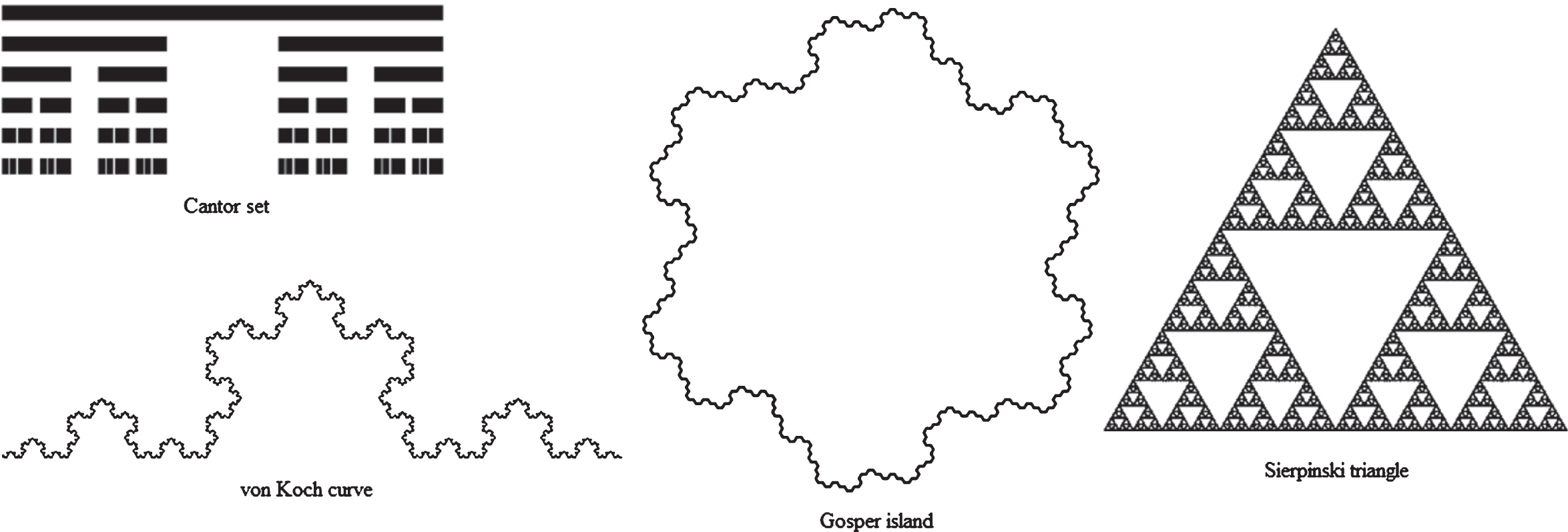
Fractal set examples.

The objective of CB mechanism is to generate self-similar neighbors that retain the good chunks of the current solution and which are different enough. It must be noted that CB mechanism is not developed for a specific problem type. It is designed as a general mechanism which can be used for any combinatorial problem where a solution point can be represented by permutation encoding. TSP and QAP are chosen to be test problems because they exhibit very different characteristics as optimization problems. When solution spaces of both problems are considered, solution space of TSP has a steep landscape and the search benefits from drastic changes in the neighborhood whilst solution space of QAP has a flat landscape and the search benefits from subtle changes in the neighborhood.

The following literature on studies of designing and improving upon novel neighbor generation mechanisms shows that the research is very limited in the area. Generally, either the existing mechanisms or their combinations are used in heuristic algorithms.

[22] compared six separate neighbor generation mechanisms for TSP, QAP and flow shop scheduling problem to investigate simulated annealing (SA) application to combinatorial optimization problems that are suited to permutation encoding. The compared mechanisms are; (1) swapping two elements on consecutive positions (consecutive swap), (2) swapping two elements on any random positions (general swap), (3) inserting a random element into a random position (general insertion), (4) changing the positions of a subsequence of elements randomly (block insertion), (5) reversing the positions of a subsequence of elements randomly (block reversion), (6) reversing the positions of a subsequence of elements randomly and/or inserting a subsequence of elements into another random position (block reversion and/or block insertion). They concluded that different methods are suitable for different problem types such that the 6^th, 4^th and 2^nd mechanisms are the best for TSP, flow-shop scheduling and QAP, respectively.

Similar neighbor generation mechanisms analyzed in [22] were also considered by [4] to show the effects of neighbor generation mechanisms on the performance of Tabu Search. The proposed Tabu Search algorithm alternates between insertion, block insertion, or swap mechanisms randomly. The purpose is to balance exploration and exploitation for solving the permutation flow shop scheduling problem. The proposed approach outperforms the compared algorithms in terms of speed and performance. Also, [15] tested the performance of the same neighboring mechanisms embedded into a hybridization of SA, LS and genetic algorithms to solve flow shop scheduling problem and the random swap mechanism was selected as the best mechanism as a result of the experimentation.

[7] presented iterated LS, SA and their hybridization to solve scheduling and transportation problems simultaneously in a job shop environment. Swap and insertion are used as neighbor generation mechanisms in the presented heuristics. However, a method called neighborhood reduction is added to the mechanisms in which the size of the neighborhood is decreased by some predefined rules. The experiments are done by using swap, reduced swap, insertion, reduced insertion, and reduced swap and insertion. They conclude that using both reduced swap and insertion gives the best performance.

[23] designed a neighborhood structure and embedded it into the SA algorithm to solve high school timetabling problem. In the study, neighbors are generated by using the swap mechanism between time slots, instead of assignments which is the usual option. After performing computational tests on two sets of benchmark instances, they concluded that their heuristic performs better than the existing methods.

[3] aimed to compare both single solution-based heuristics (LS, SA, Tabu Search, Variable Neighborhood Search) and population-based heuristics (Genetic Algorithm, Memetic Algorithm) in their experiments. They stated that the most commonly used neighbor generation mechanism in QAP studies is swap mechanism and for that reason they used swap for all the single solution-based algorithms. Their results showed that there is no single best algorithm for solving QAP and different instances respond well to different heuristics.

There are various neighbor generation mechanisms such as r-opt [11], ejection chains [8], stem-and-cycle [9] that are designed specifically for TSP and cannot be generalized to other combinatorial problems. However, most of the studies in the literature use swap for QAP (see for examples; [2 , 20]) meaning there is not a neighbor generation mechanism specific to QAP. On the other hand rthe interest of the present study lies within generalized neighbor generation mechanisms not problem specific ones. In this study rwe designed and tested variants of CB method and used them to solve both TSP and QAP.

In the 2^nd section, the test problems (TSP, QAP) and search heuristics (LS, SA) in which CB method is embedded are explained briefly. CB method is described in the 3^rd section in detail. An experimental study conducted for several design issues of CB method and a comparative study of CB mechanisms with swap and insertion neighbor generation mechanisms is presented in Section 4. Finally, the conclusions are discussed in the last section.

2 Test problems and search heuristics

TSP and QAP are frequently used in the literature to analyze performances of new methods since these problems are easy to code but hard to solve. TSP is a popular problem with the metaphor of a salesman starting from a city, has to visit n cities (from a known list of cities) exactly once and then he has to return to the first city. He wants to select an order to visit the cities with minimum total distance travelled. In QAP, there are a set of facilities and a set of locations. The distances between locations and the flows between the facilities are fixed. The objective is to assign each facility to each location while minimizing the sum of the products between flows and distances. Interested readers are referred to 18] and [6] for further information on TSP and QAP including their mathematical descriptions.

The objective of this study is to show the performance of CB method by embedding it into various search algorithms rather than to design a sophisticated heuristic algorithm for the selected test problems. For this purpose, basic LS and SA heuristics are selected to embed CB method into. These heuristics are explained briefly in the next subsections.

2.1 Local search

LS is the most basic single solution-based heuristic. LS starts from x, which is a single feasible initial solution. At each iteration, N (x) (whole or partial neighborhood of a solution) which is the set of neighbor solutions x′ is investigated. The search proceeds from one feasible solution to a better feasible solution by using a neighbor generation mechanism until a locally optimal solution is reached. The new current solution can be selected by one of the following strategies: best improvement, first improvement and random selection [21]. In this study, the best improvement is used as the selection strategy and the algorithm stops at the first time there is no better solution among the explored neighbors.

2.2 Simulated annealing

SA is a simple and effective stochastic heuristic proposed by [10]. SA algorithm accepts better solutions as they come along. However, in the course of the run, if the algorithm encounters a worse solution, it accepts that solution with a probability of $p (Δ f, T) = e^{(\frac{- Δ f}{T})}$ . In this formula, Δf = f (x′) - f (x) where f is the minimization objective function, x and x′ are the current and neighbor solutions, respectively, and T is the temperature parameter. T is decreased according to a cooling schedule which is geometric cooling schedule in this study: T_(i+1) = T_(i) × α. In the literature, α is generally set to a value between 0.85 to 0.99. It is also important to mention that the cooling schedule should provide an equilibrium state (δ) at each temperature. In the selected cooling schedule, δ is the number of iterations which temperature T remains the same before updating it while δ value is generally used as a function of n. Details of SA can be found in [10].

3 Cantor set based neighbor generation mechanism

Fractals are described by Mandelbrot [12]. Although there is no specific definition for what a fractal is, one of the definitive characteristics of fractals is that they have repetitive structures at different length scales (statistical self-similarity). One of the famous fractals is a cantor set which was discovered by Smith in 1870s and it was introduced to the world by Cantor in 1880s. Cantor sets can be built by recursive algorithms which is the inspiration of the proposed CB method. The steps in the recursive algorithm that generates a deterministic cantor is described in Figure 2 [1].

Fig. 2

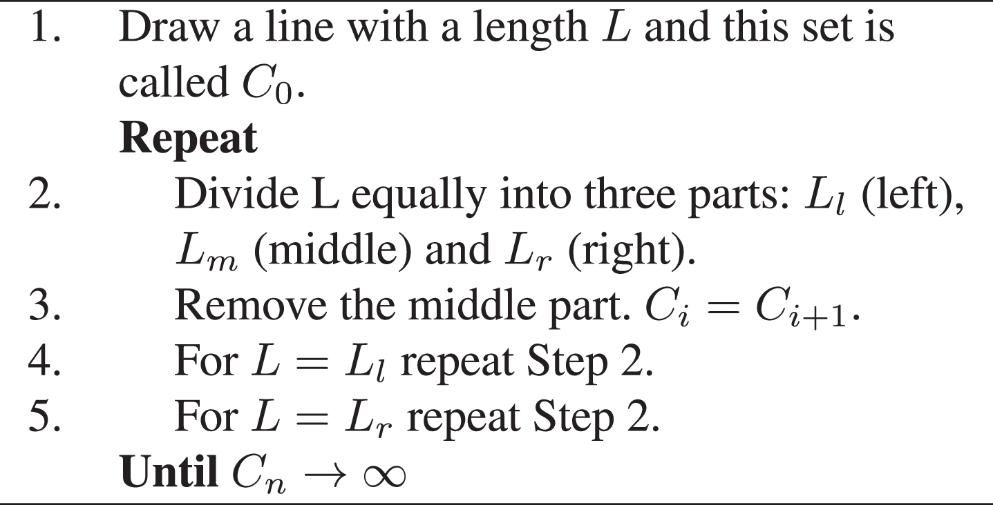
The recursive algorithm that generates a deterministic cantor set.

The deterministic generation of cantor sets is easier to explain as the intervals can be given specifically. Hence, it is easier to understand the stochastic cantor sets after observing deterministic cantor sets. In stochastic generation of cantor sets, in step 2, the line is not divided into three parts with equal lengths, but it is divided into three parts with random lengths.

In step 2 (and in the following steps), notice that the concerned part is divided into three parts and the middle sections are removed. However, if a section is removed from the solution representation, the integrity of the representation (which is the permutation of n elements) will be lost. Therefore, the dividing process is executed in CB mechanism, but the middle parts are committed to memory. CB mechanism produces similar neighbors that are different enough, by using the self-similarity aspect of fractal sets.

Figure 3 is presented to explain the structure of CB mechanism. In the initial stage (stage-0), the permutation solution representation, x = [x₁, x₂, . . . , x_n], is represented by a complete string (p₀) of size n, where n is the problem size. In stage-1, p₀ is divided into three substrings. For this purpose, a starting element, s, is systematically increased from 1 to (n - 2). For each s, an index number, m, is increased from 1 to (n - s - 1) such that the first substring (p₀₁) contains the variables [x₁, x₂, . . . , x_s], the second (p₀₂) contains [x_(s+1), x_(s+2), . . . , x_(s+m)], and finally, the last substring (p₀₃) contains [x_(s+m+1), x_(s+m+2), . . . , x_n]. For the sake of clarity, the dividing process in stage-1 is explained as follows:

Fig. 3

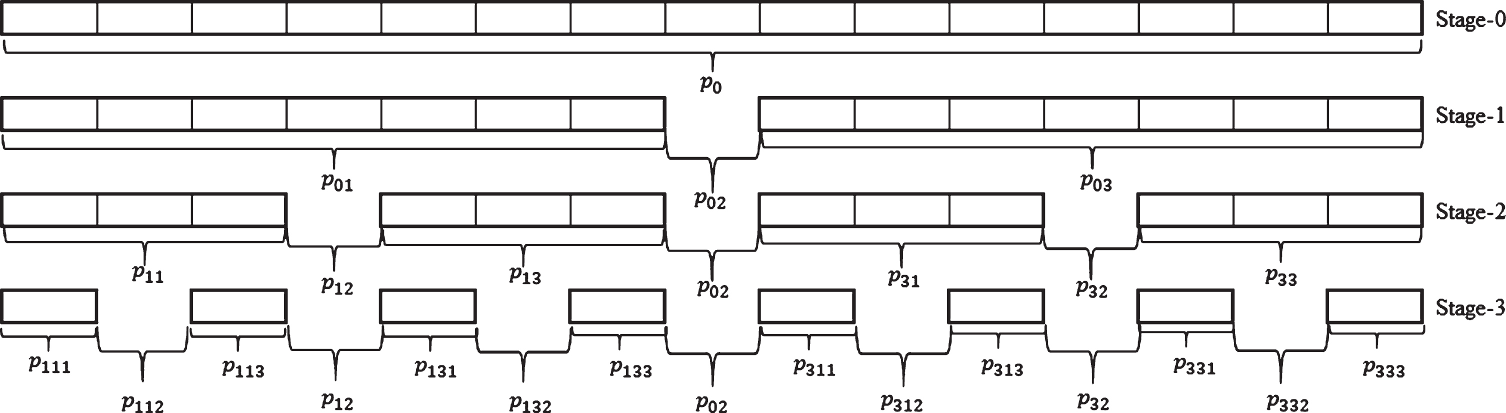
A representative figure for how substrings would look like (mid-substrings are void to improve visibility).

(1) Substring p₀₁ = [x₁, x₂, . . . , x_s] is changed for each s = 1, 2, . . . , n - 2. This means that p₀₁ always starts from x₁ and the number of elements in p₀ is increased from 1 to n - 2 sequentially. Therefore, the number of times p₀₁ is changed depends on problem size n.

(2) Substring p₀₂ always starts with the element x_s+1. The number of elements in p₀₂ is changed from 1 element, up to n - 2 elements and for each different p₀₂, p₀₃ consists of the remaining elements such that, p₀₃ = [x_s+2, . . . , x_n] for p₀₂ = [x_s+1], p₀₃ = [x_s+3, . . . , x_n] for p₀₂ = [x_s+1, x_s+2] and so on. The last possible choice for p₀₂ is x_n-1 which leads to p₀₃ = [x_n].

Notice that the dividing process explained above is also valid for stage-2 and stage-3. For stage-2, steps 1 and 2 are applied to p₀₁ and p₀₃ (left and right parts in the recursive algorithm which generates a cantor set), separately. The mid-substring (p₀₂) is never divided to maintain the self-similarity structure. From p₀₁, the substrings p₁₁, p₁₂ and p₁₃ are determined and the substrings p₃₁, p₃₂ and p₃₃ are determined from p₀₃ where p_ij means that j^th substring of string-i. In stage-3, steps 1 and 2 are applied to p₁₁, p₁₃, p₃₁ and p₃₃ separately. Hence, the substrings p₁₁₁, p₁₁₂ and p₁₁₃ are generated from p₁₁, the substrings p₁₃₁, p₁₃₂ and p₁₃₃ are generated from p₁₃, the substrings p₃₁₁, p₃₁₂ and p₃₁₃ are generated from p₃₁, and finally the substrings p₃₃₁, p₃₃₂ and p₃₃₃ are generated from p₃₃.

Once the substrings in the respective stages are obtained, the neighbors are generated using the permutations of the concerned substrings. In this study, two different permutation schemes are designed to obtain the neighborhood of a given solution. The first scheme provides big perturbations on the solution while the second scheme provides small perturbations as explained in the next two subsections.

3.1 Neighbor generation schemes

In the first scheme, the neighbor sets of each stage are generated by permutating appropriate substrings. In stage-1, p_ij is permutated for each j = 1, 2, 3. In stage-2, p_kj for each k = 1, 3 (left and right substrings) separately while keeping the other substrings in the same position. Similarly, each substrings p_ij, but the mid-substrings (p_i2), are divided into three parts, t = 1, 2 and 3, to create substrings, p_ijt, in stage-3. The neighbor set of stage-3 is created by the permutations of substrings p_ijt for each pair of i, j separately while fixing the other substrings in the same position creating (3 ! -1) neighbors for each pair.

Figure 4 shows a visual representation of scheme-1. It should be noted that mid-substrings (p_i2, i = 0, 1, 3) are not divided into subparts and also, the permutations in each stage are obtained using only the three adjacent substrings for the sake of self-similarity structure of cantor sets.

Fig. 4

A visual representation of neighbor generation using scheme-1 (left hand side) and scheme-2 (right hand side).

In the second scheme, dividing of the substrings is the same as the previous application but the permutation procedure differs in that permutations are only done between substrings p_i2 and p_ij2 without changing the position and order of other substrings as explained in Figure 4 visually.

A pseudo code that shows the general structure of CB mechanism is presented in Figure 5 where f (x) is the minimization objective function.

Fig. 5

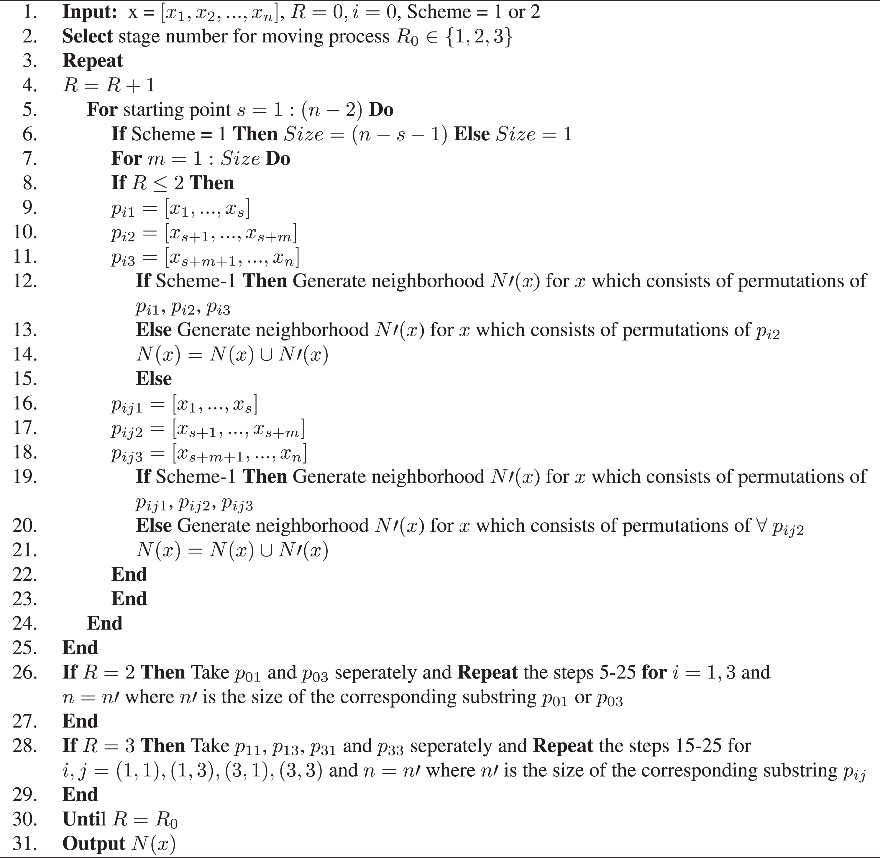
Pseudo code of CB method.

The interested reader can access three numerical examples for the neighbor generation in stage-1, stage-2 and stage-3 in http ://bit . ly/2LMdSwW.

3.2 Design choices used in CB mechanism

Several choices in the design of CB mechanism are analyzed to increase the effectiveness and the efficiency. These design issues are especially important to decrease the memory space and run-time required by the mechanism. Pre-experiments showed that the following design choices may affect the performance and run-time of the mechanism: choosing the best solution when advancing to the next stage, the number of stages (1, 2 or 3) that CB mechanism proceeds, reverse ordering of substrings, neighbor generation schemes (scheme-1 and scheme-2).

A pre-experimental study was made by implementing CB mechanism on several TSP and QAP instances in varying sizes considering all possible choices of the mentioned design issues and some other choices were abandoned as they gave unsatisfactory performance. The remaining design choices are chosen to be presented in this study, since they have already outperformed the other alternatives in terms of effectiveness and/or efficiency.

Design issue to deal with exponential increasing in the number of neighbors: It is obvious that the number of neighbors increases exponentially as the number of stages increases since each neighbor created in each stage is an input string to the next stage in the general structure of CB mechanism as illustrated in Figure 4. To avoid this exponential increment, the neighbor that gives the minimum objective function value in the previous stage is picked and the process of the next stage is applied to the selected neighbor instead of complete set of neighbors of just previous stage. For example, for an n = 100 problem, the algorithm gives very similar results 13 - 15 times faster when this design choice is implemented.

Design issue of all stages: CB mechanism can proceed until stage-1, stage-2 or stage-3 and therefore, the maximum number of the stages is another design issue. To improve the exploitation capability of CB, additional neighbors are generated using the reverse orders of the elements in the mid-substrings.

Straight ordering and reverse ordering: Once the solution is divided into substrings as explained in Section 3 and illustrated in Figure 3, each mid-substring p_i2 and p_ij2 is used in the neighbor generation scheme-1 or scheme-2 in two different ways. The first way, called straight ordering, means that the mid-substrings are used directly. On the other hand, reverse ordering changes the sequence of the elements in the mid-substrings and use them in reverse order.

3.3 Variations of CB mechanism used in this study

Originally, it is possible to generate neighbors by using the general idea behind the method. However, there are many options that can make the algorithm too slow. Therefore, in consideration of the design choices, 3 alternative CB variations are presented: CB-1, CB-2 and CB-3.

CB-1: Proceed until stage-2, straight ordering, scheme-2.

CB-2: Proceed until stage-2, reverse ordering, scheme-1

CB-3: Proceed until stage-3, reverse ordering, scheme-1

4 Experimental study

In the computational tests, MATLAB 2017 was used for coding where the hardware was an Intel i5-7200U CPU @ 2,50GHz 2,70 GHz. The benchmark instances are taken from TSPLIB [17] and QAPLIB [5]. For the experiments, every mechanism was embedded into LS and SA algorithms separately and they were run 30 times starting from the same initial solution using these test instances.

In Table 1 CB-1, CB-2, and CB-3 are compared in terms of solution quality and the total number of neighbors generated until the termination condition of LS procedure is met while solving TSP instances. The same comparisons are given in Table 2 for solving QAP instances. SA results for number of generated neighbors are not reported here because the number of generated neighbors depends on the cooling schedule not the neighbor generation mechanism itself.

Table 1
Percentage deviations from the best known solution (DBKS^) and number of neighbors generated (NNG^) by CB variations for TSP

CB-1 CB-2 CB-3

Problem Set DBKS^* NNG^* DBKS^* NNG^* DBKS^* NNG^*

krob100 72.4 3.2 × 10⁶ 2.5 1.2 × 10⁷ 2.63 1.0 × 10⁷

lin105 79.58 3.2 × 10⁶ 1.99 2.0 × 10⁷ 2.77 1.3 × 10⁷

bier127 43.2 5.2 × 10⁶ 2.59 3.7 × 10⁷ 3.72 2.3 × 10⁷

ch130 71.39 5.9 × 10⁶ 2.47 4.1 × 10⁷ 3.83 2.5 × 10⁷

kroa150 84.45 9.6 × 10⁶ 2.88 6.2 × 10⁷ 3.33 3.9 × 10⁷

krob150 92.5 1.1 × 10⁷ 2.24 6.4 × 10⁷ 3.38 3.7 × 10⁷

ch150 75.82 1.0 × 10⁷ 3.19 6.0 × 10⁷ 3.58 4.1 × 10⁷

d198 118.27 2.9 × 10⁷ 1.6 1.5 × 10⁸ 1.86 1.0 × 10⁸

kroa200 105.44 2.6 × 10⁷ 3.22 1.6 × 10⁸ 3.73 9.5 × 10⁷

krob200 99.92 2.6 × 10⁷ 4.28 1.6 × 10⁸ 4.19 1.0 × 10⁸

gil262 102.07 6.5 × 10⁷ 4.2 3.7 × 10⁸ 4.51 2.4 × 10⁸

pr264 305.88 6.2 × 10⁷ 4.92 4.1 × 10⁸ 5.53 2.2 × 10⁸

pr299 125.99 1.0 × 10⁸ 4.36 5.8 × 10⁸ 4.6 3.8 × 10⁸

lin318 139.1 1.2 × 10⁸ 3.29 6.8 × 10⁸ 3.59 4.2 × 10⁸

fl417 489.05 3.1 × 10⁸ 1.96 1.6 × 10⁹ 2.26 1.0 × 10⁹

	CB-1	CB-2	CB-3
krob100	72.4	3.2 × 10⁶	2.5	1.2 × 10⁷	2.63	1.0 × 10⁷
lin105	79.58	3.2 × 10⁶	1.99	2.0 × 10⁷	2.77	1.3 × 10⁷
bier127	43.2	5.2 × 10⁶	2.59	3.7 × 10⁷	3.72	2.3 × 10⁷
ch130	71.39	5.9 × 10⁶	2.47	4.1 × 10⁷	3.83	2.5 × 10⁷
kroa150	84.45	9.6 × 10⁶	2.88	6.2 × 10⁷	3.33	3.9 × 10⁷
krob150	92.5	1.1 × 10⁷	2.24	6.4 × 10⁷	3.38	3.7 × 10⁷
ch150	75.82	1.0 × 10⁷	3.19	6.0 × 10⁷	3.58	4.1 × 10⁷
d198	118.27	2.9 × 10⁷	1.6	1.5 × 10⁸	1.86	1.0 × 10⁸
kroa200	105.44	2.6 × 10⁷	3.22	1.6 × 10⁸	3.73	9.5 × 10⁷
krob200	99.92	2.6 × 10⁷	4.28	1.6 × 10⁸	4.19	1.0 × 10⁸
gil262	102.07	6.5 × 10⁷	4.2	3.7 × 10⁸	4.51	2.4 × 10⁸
pr264	305.88	6.2 × 10⁷	4.92	4.1 × 10⁸	5.53	2.2 × 10⁸
pr299	125.99	1.0 × 10⁸	4.36	5.8 × 10⁸	4.6	3.8 × 10⁸
lin318	139.1	1.2 × 10⁸	3.29	6.8 × 10⁸	3.59	4.2 × 10⁸
fl417	489.05	3.1 × 10⁸	1.96	1.6 × 10⁹	2.26	1.0 × 10⁹

Table 2

Percentage deviations from the best known solution (DBKS^*) and number of neighbors generated (NNG^*) by CB variations for QAP

	CB-1		CB-2		CB-3
Problem Set	DBKS^*	NNG^*	DBKS^*	NNG^*	DBKS^*	NNG^*
Tai25b	12.62	2.5 × 10⁴	25.83	3.9 × 10⁴	16.91	1.6 × 10⁵
Chr25a	50.95	2.5 × 10⁴	134.41	2.7 × 10⁴	92.17	1.2 × 10⁵
Nug27	3.6	3.5 × 10⁴	13.98	3.1 × 10⁴	6.98	1.8 × 10⁵
Tho30	3.71	5.7 × 10⁴	12.42	7.3 × 10⁴	6.96	2.6 × 10⁵
Nug30	2.79	5.9 × 10⁴	11.75	6.9 × 10⁴	6.76	2.5 × 10⁵
Esc32h	2.16	5.1 × 10⁴	11.9	5.6 × 10⁴	5.54	2.6 × 10⁵
Esc32d	4.93	4.5 × 10⁴	20.23	5.2 × 10⁴	13.8	2.5 × 10⁵
Tho40	3.01	1.5 × 10⁵	15.08	2.1 × 10⁵	7.8	7.6 × 10⁵
Wil50	1.21	3.3 × 10⁵	5.4	5.4 × 10⁵	2.54	1.5 × 10⁶
Tai60a	3.37	5.8 × 10⁵	10.17	6.4 × 10⁵	7.49	3.1 × 10⁶
Tai60b	5.41	5.9 × 10⁵	17.53	1.2 × 10⁶	13.46	4.0 × 10⁶
Tai80b	4.96	1.4 × 10⁶	13.63	3.2 × 10⁶	10.65	1.2 × 10⁷
Lipa90b	21.07	2.3 × 10⁶	25.76	2.7 × 10⁶	24.06	1.2 × 10⁷
Tai100b	3.9	3.3 × 10⁶	20.32	4.9 × 10⁶	10.82	2.7 × 10⁷
Wil100	0.84	3.9 × 10⁶	4.58	6.5 × 10⁶	2.42	1.7 × 10⁷

For TSP, CB-2 and CB-3 generates significantly more neighbors than CB-1. However, CB-2 gives the best results among the mechanisms in terms of solution quality. Hence, it is thought that the number of neighbors generated by the mechanisms is a result of their design and performance does not get affected by it. This observation is supported by the QAP results that can be observed in Table 2. Even though CB-3 generates significantly more neighbors than CB-1 and CB-2, CB-1 gives the best performance.

4.1 Comparison of CB mechanism with classical neighbor generation mechanisms

CB-1, CB-2 and CB-3 are compared to classical swap and insertion mechanisms in terms of effectiveness and efficiency. In addition, since SA heuristic had to be tuned before actual runs, test runs were executed for the sake of parameter tuning.

4.1.1 Parameter tuning for SA

In this study, a static parameter set, which is determined by a factorial design is used for SA. Parameters of the geometric cooling schedule, which is one of the widely used schedules, and the levels of each parameter determined by pre-experiments are given as follows for both TSP and QAP:

Cooling rate (α): 0.90, 0.95, 0.99

Initial temperature (T₀): n, 5n, 50n, 100n

Ending temperature (T_f): 0.1n, 0.01n, 0.001n

Equilibrium state (δ): n, 5n, 10n, 15n

Three benchmark instances (small, medium and large sized) of TSP and QAP are chosen for the experiments. Each possible parameter combination is tested 30 times. For TSP, the following set of parameters is determined: 1. α = 0.99, 2. T₀ = 5n, 3. T_f = 0.001n, 4. δ = 15n. Parameter set is found as 1. α = 0.99, 2. T₀ = 100n, 3. T_f = 0.001n, 4. δ = 5n for QAP.

4.2 Statistical tests

To provide statistical inferences from the comparison of the mechanisms, SPSS-24 was used as a statistical analyzer. Tables 3 and 4 show the descriptive statistics of percentage deviation from the best-known solutions for TSP and QAP, respectively.

Table 3
Descriptive statistics of the mechanisms in terms of percentage deviation from the best-known solution for TSP

N Mean Std. Deviation Minimum Maximum

Local Search

Swap 450 185.86 165.31 40.34 890.47

Insertion 450 59.14 33.87 17.94 196.8

CB-1 450 133.67 113.36 28.76 585.57

CB-2 450 3.05 1.7 0.03 13.41

CB-3 450 3.57 1.8 0 13.99

Simulated Annealing

Swap 450 545.01 720.51 8.74 3032.87

Insertion 450 532.11 718.15 0.27 2999.82

CB-1 450 22.24 12.78 3.90 82.19

CB-2 450 3.57 2.55 0 16.95

CB-3 450 3.84 2.61 0 15.65

	N	Mean	Std. Deviation	Minimum	Maximum
Local Search
Swap	450	185.86	165.31	40.34	890.47
Insertion	450	59.14	33.87	17.94	196.8
CB-1	450	133.67	113.36	28.76	585.57
CB-2	450	3.05	1.7	0.03	13.41
CB-3	450	3.57	1.8	0	13.99
Simulated Annealing
Swap	450	545.01	720.51	8.74	3032.87
Insertion	450	532.11	718.15	0.27	2999.82
CB-1	450	22.24	12.78	3.90	82.19
CB-2	450	3.57	2.55	0	16.95
CB-3	450	3.84	2.61	0	15.65

Table 4

Descriptive statistics of the mechanisms in terms of percentage deviation from the best-known solution for QAP

	N	Mean	Std. Deviation	Minimum	Maximum
Local Search
Swap	450	10.39	15.33	0	98.74
Insertion	450	29.36	39.78	3.27	222.71
CB-1	450	8.3	13.25	0	74.03
CB-2	450	22.87	31.13	3.58	174.45
CB-3	450	15.22	21.99	0.72	123.55
Simulated Annealing
Swap	450	6.20	8.56	0	48.95
Insertion	450	21.42	26.31	2.15	135.99
CB-1	450	6.71	10.10	0	49.37
CB-2	450	17.37	22.49	1.83	128.13
CB-3	450	16.38	19.94	1.37	104.16

For TSP, the results given in Table 3 show that when LS is used, CB-2 and CB-3 mechanisms perform similarly well compared to the other mechanisms in terms of percentage deviation from the best-known solution. Although, CB-2 is slightly more robust than CB-3, it greatly outperforms the other mechanisms. When SA is used, CB-2 and CB-3 are again the best mechanisms by far, albeit CB-2 is slightly better than CB-3. CB-1 is not suitable for TSP at all, giving similar results with insertion and swap. For QAP, the results given in Table 4 show that when LS is used, CB-1 mechanism is the best compared to the others in terms of percentage deviation from the best-known solution. CB-1 is also more robust than other mechanisms since it has a lower standard deviation. Swap is the best mechanism when embedded into SA and CB-1 exhibits a similar performance with swap in terms of percentage deviation from the best-known solution. CB-2 is not suitable for QAP at all, giving similar results with insertion mechanism.

In addition, Friedman Test is applied to compare the mechanisms for TSP and QAP, separately, by using percentage deviations from the best-known solution data and the results are presented in Table 5. Friedman test is a ranking method based non-parametric statistical test that is used to compare matched groups. While interpreting the results, the mechanism that has the lowest ranking is considered the best while the mechanism that has the highest ranking is considered the worst as the resulting deviation is desired to be zero in the ideal case. For TSP, CB-2 embedded into LS and SA is the best. For QAP, CB-1 embedded into LS and swap embedded into SA are the best. These results support the interpretations observed from Tables 3 and 4.

Table 5

Friedman Test using percentage of deviation from the best-known solution for TSP and QAP

Mean Rank
	Local Search					Simulated Annealing
	Swap	Insertion	CB-1	CB-2	CB-3	Swap	Insertion	CB-1	CB-2	CB-3
TSP	4.94	3.01	4.05	1.40	1.60	4.94	3.84	3.21	1.46	1.56
QAP	1.92	4.69	1.32	4.17	2.90	1.51	4.42	1.56	3.88	3.62

In Tables 6 and 7, run-time (average time required until a local optimum is met) is compared on each instance for TSP and QAP, respectively. For each instance, swap is the fastest mechanism embedded into both LS and SA for solving TSP. Because swap is a simple mechanism, its computer time requirement is less than that of the other mechanisms. However, its simplicity fails to find high quality solutions as reported in Table 3. On the other hand, CB-3 is the slowest mechanism when LS is used while CB-2 is the slowest when SA is used to solve TSP instances. For QAP instances, swap and insertion perform in similar run-times when embedded into both LS and SA. These mechanisms are faster than CB mechanisms on QAP instances. CB-3 requires more computational time compared to the other mechanisms.

Table 6

Run-time (in seconds) for TSP

	Local Search					Simulated Annealing
Problem Set	Swap	Insertion	CB-1	CB-2	CB-3	Swap	Insertion	CB-1	CB-2	CB-3
krob100	1.7	9.6	11.3	8.3	32.6	23.5	27.0	48.3	113.0	99.4
lin105	2.0	10.5	14.5	9.4	38.4	26.6	32.1	50.2	99.6	104.9
bier127	4.0	19.0	23.2	16.2	74.0	34.0	35.8	56.0	118.5	126.3
ch130	4.5	21.7	26.8	18.3	78.9	32.4	38.5	60.1	126.1	137.7
kroa150	9.1	40.8	51.0	29.1	127.5	36.3	43.3	67.4	144.1	151.8
ch150	8.8	37.7	53.7	27.9	121.5	34.4	39.6	70.5	141.9	151.4
krob150	8.1	34.8	45.5	26.4	138.0	38.4	46.1	79.0	156.3	159.6
d198	23.1	107.5	158.0	71.5	369.5	51.2	60.8	96.3	217.2	187.0
krob200	23.2	112.7	128.6	72.1	351.1	50.5	61.4	92.6	215.7	186.9
kroa200	23.9	105.5	129.4	70.1	380.4	47.4	55.6	92.3	218.4	184.9
gil262	62.6	273.7	421.7	164.5	961.7	82.0	99.3	154.6	383.8	296.2
pr264	63.5	271.3	429.3	182.2	881.4	67.2	80.5	119.0	337.3	251.6
pr299	115.3	475.6	679.4	257.5	1447.8	79.8	90.8	135.5	288.8	283.2
lin318	134.3	548.8	848.0	302.0	1659.2	83.8	96.9	147.3	341.7	304.6
fl417	440.6	1750.2	2752.9	721.1	4362.8	119.4	138.4	211.7	471.0	422.2

Table 7

Run-time (in seconds) for TSP

	Local Search					Simulated Annealing
Problem Set	Swap	Insertion	CB-1	CB-2	CB-3	Swap	Insertion	CB-1	CB-2	CB-3
Tai25b	0.1	0.1	0.3	0.9	2.4	3.1	3.9	6.6	11.7	10.5
Chr25a	0.03	0.05	0.3	0.5	1.9	3.1	3.4	5.9	14.1	10.8
Nug27	0.1	0.1	0.4	0.6	3.2	4.4	4.2	7.5	16.0	13.0
Tho30	0.1	0.2	0.8	1.6	4.8	4.3	4.5	7.1	16.8	14.0
Nug30	0.1	0.1	0.9	1.5	4.7	5.3	5.2	8.5	18.7	16.8
Esc32h	0.1	0.1	0.8	1.3	5.1	8.0	6.6	12.0	22.3	22.8
Esc32d	0.1	0.1	0.7	1.2	4.9	8.2	7.9	15.8	26.1	31.4
Tho40	0.4	0.6	3.6	6.9	20.2	7.6	7.3	12.1	23.0	27.4
Wil50	1.5	2.0	11.6	23.5	55.0	1.5	2.0	23.2	36.7	38.6
Tai60a	2.1	2.1	28.8	43.0	159.1	2.1	2.1	28.5	42.1	43.4
Tai60b	3.8	4.5	33.0	73.0	205.9	3.8	4.5	30.1	43.5	43.6
Tai80b	17.6	15.7	114.1	279.4	1063.7	17.6	15.7	50.6	62.2	71.4
Lipa90b	16.5	15.3	220.4	296.8	1197.2	44.7	46.3	56.0	77.4	94.8
Tai100b	59.1	53.2	416.9	634.3	3585.7	59.1	53.2	83.5	99.0	109.6
Wil100	59.0	59.2	502.2	866.9	2334.8	79.8	79.1	97.5	115.0	120.3

Finally, Figures 6 and 7 are presented to visualize the performance comparisons between CB mechanisms. Figure 6 illustrates the solution quality performances of CB-1, CB-2, and CB-3 using LS and SA heuristics for TSP instances while similar illustrations are given in Figure 7 for QAP instances. A curious observation regarding Figure 6 is that CB-2, which is the best mechanism for solving TSP, performs better embedded into SA for n < 150 and CB-2 performs better when embedded into LS for n > 150. A similar situation can be observed for CB-3 results as well.

Fig. 6

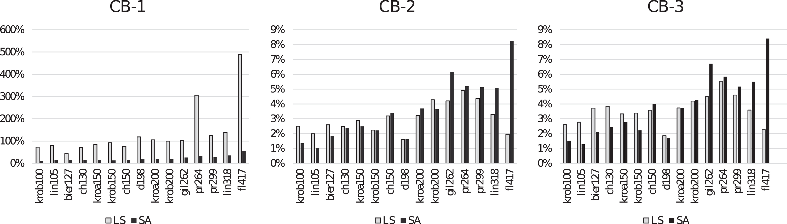
Comparison of CB-1, CB-2, CB-3 on TSP instances in terms of deviation from the best known solution.

Fig. 7

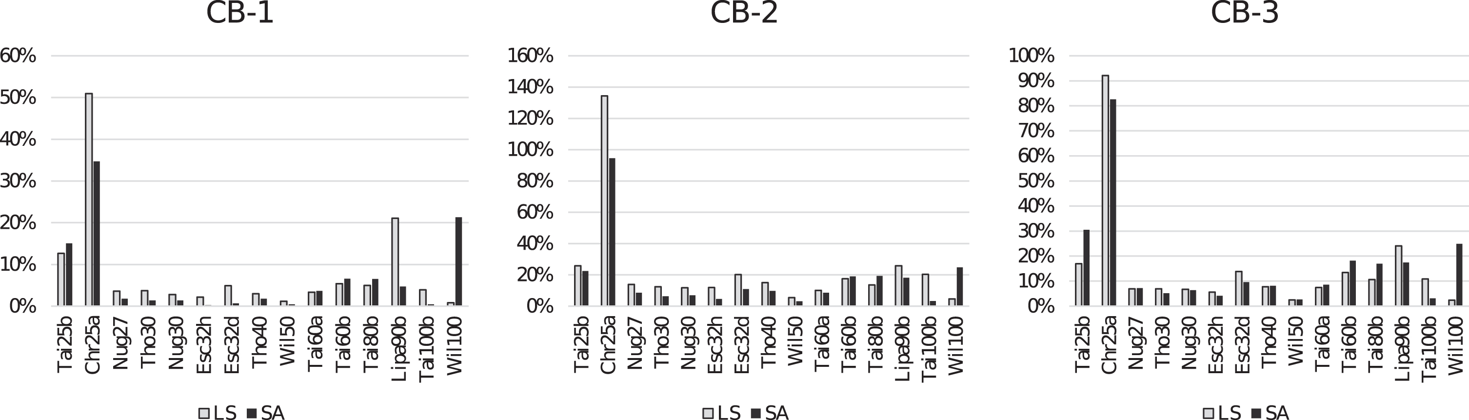
Comparison of CB-1, CB-2, CB-3 on QAP instances in terms of deviation from the best known solution.

5 Conclusions

In this study, a novel neighbor generation mechanism, called CB, to enhance the performance of single solution-based heuristics is described and improved. CB mechanism is inspired by the recursive algorithm that creates stochastic cantor sets which is one of the well-known fractal sets. Several issues in the design of CB mechanism are investigated for the purpose of finding a mechanism that performs well on TSP and QAP which have differentiating characteristics. Considering the design issues, three variations of CB mechanism are created: CB-1, CB-2 and CB-3. The variations of CB are compared with classical move operators, swap and insertion, on benchmark instances of TSP and QAP. The results present that among CB variations, CB-2 embedded into LS and SA to solve TSP outperforms swap and insertion mechanisms in terms of solution quality while CB-3 exhibits the next best performance after CB-2. For QAP, on the other hand, CB-1 embedded into LS is superior to both swap and insertion, however, the solution qualities generated by CB-1 and swap mechanisms are very close to each other. This proves that, for TSP, big jumps in the search space provided by CB-2 and CB-3 give better results while a more delicate approach with small jumps created by CB-1 is necessary for QAP. In other words, it is showed that different variations of CB mechanism are able to deal with different characteristics of TSP and QAP where the landscapes in TSP instances contain deep valleys and the landscapes in QAP instances have flat valleys. On the other hand, CB mechanism is always slower than swap and insertion mechanisms in terms of run-time, even though it requires a reasonable amount of run-time to solve moderate or larger sized instances.

The major contribution of the presented study is the introduction of a novel neighbor generation mechanism because the literature mainly consists of traditional swap and insertion mechanisms or their variations. Another important insight obtained from the experimental study is that CB-3 gives consistently good results when solving both TSP and QAP despite of their contrary characteristics in their landscapes. This is an encouraging result since there is not a common neighbor generation mechanism which performs well for both TSP and QAP.

As a future study, CB mechanism will be improved further in terms of run-time and as a more efficient generalized neighbor generation mechanism. It also will be applied to different benchmark or real-life combinatorial optimization problems to show its applicability and to enhance its usage in the operational research community.

References

Alligood

K.T.

, Sauer

T.D.

and Yorke

J.A.

, Chaos, Springer New York, 1996, pp. 149–160.

Angel

and Zissimopoulos

, On the landscape ruggedness of the quadratic assignment problem, Theoretical computer science 263(1-2) (2001), 159–172.

Beham

, Affenzeller

and Pitzer

, Metaheuristic Algorithms for the Quadratic Assignment Problem: Performance and Comparison, In Innovative Technologies in Management and Science, Springer Cham, 2015, pp. 171–190.

Ben-Daya

and Al-Fawzan

, A tabu search approach for the flow shop scheduling problem, European journal of operational research 109(1) (1998), 88–95.

Burkard

R. E.

, Çela

, Karisch

S.E.

and Rendl

, QAPLIB–A quadratic assignment problem library, 2010.

Cela

, The quadratic assignment problem: theory and algorithms (Vol. 1). Springer Science and Business Media, 2013.

Deroussi

, Gourgand

and Tchernev

, A simple metaheuristic approach to the simultaneous scheduling of machines and automated guided vehicles, International Journal of Production Research 46(8) (2008), 2143–2164.

Glover

, Multilevel tabu search and embedded search neighborhoods for the traveling salesman problem, Graduate School of Business, University of Colorado, 1991.

Glover

, Ejection chains, reference structures and alternating path methods for traveling salesman problems, Discrete Applied Mathematics 65(1-3) (1996), 223–253.

10.

Kirkpatrick

, Gelatt

C.D.

and Vecchi

M.P.

, Optimization by simulated annealing,, Science 220 (1983), 671–680.

11.

Lin

and Kernighan

B.W.

, An effective heuristic algorithm for the traveling-salesman problem, Operations research 21(2) (1973), 498–516.

12.

Mandelbrot

B.B.

, The fractal geometry of nature, W. H. Freeman and Company, 1983.

13.

Mills

, Tsang

and Ford

, Applying an extended guided local search to the quadratic assignment problem, Annals of Operations Research 118(1-4) (2003), 121–135.

14.

Misevičius

, An intensive search algorithm for the quadratic assignment problem, Informatica 11(2) (2000), 145–162.

15.

Nearchou

A.C.

, A novel metaheuristic approach for the flow shop scheduling problem, Engineering Applications of Artificial Intelligence 17(3) (2004), 289–300.

16.

Öztürk

and Alabaş-Uslu

Ç.

, A Novel Neighborhood Generation Method for Heuristics and Application to Traveling Salesman Problem, In: C. Kahraman, S. Cebi, S. Cevik Onar, B. Oztaysi, A. Tolga, I. Sari. (eds) Intelligent and Fuzzy Techniques in Big Data Analytics and Decision Making. INFUS 2019. Advances in Intelligent Systems and Computing, 2020, vol 1029. (pp. 1215–1221). Springer, Cham.

17.

Reinelt

, TSPLIB–A traveling salesman problem library, ORSA journal on computing 3(4) (1991), 376–384.

18.

Shmoys

D.B.

, The traveling salesman problem: a guided tour of combinatorial optimization, (Vol. 3, pp. 1–463). In: E.L. Lawler, J.K. Lenstra, and A.R. Kan (Eds.). New York, Wiley, 1985.

19.

St”utzle

, Iterated local search for the quadratic assignment problem, European Journal of Operational Research 174(3) (2006), 1519–1539.

20.

Taillard

, Robust taboo search for the quadratic assignment problem, Parallel Computing 17(4-5) (1991), 443–455.

21.

Talbi

E.G.

, Metaheuristics: from design to implementation, John Wiley and Sons, New Jersey, 2009, pp. 88–90.

22.

Tian

, Ma

and Zhang

D.M.

, Application of the simulated annealing algorithm to the combinatorial optimisation problem with permutation property: An investigation of generation mechanism, European Journal of Operational Research 118(1) (1999), 81–94.

23.

Zhang

, Liu

, M’Hallah

and Leung

S.C.

, A simulated annealing with a new neighborhood structure based algorithm for high school timetabling problems, European Journal of Operational Research 203(3) (2010), 550–558.