Data-driven disruption prediction in GOLEM Tokamak using ensemble classifiers

Abstract

A robust disruption prediction system is mandatory in a Tokamak control system as the disruption can cause malfunctioning of the plasma-facing components and impair irrecoverable structural damage to the vessel. To mitigate the disruption, in this article, a data-driven based disruption predictor is developed using an ensemble technique. The ensemble algorithm classifies disruptive and non-disruptive discharges in the GOLEM Tokamak system. Ensemble classifiers combine the predictive capacity of several weak learners to produce a single predictive model and are utilized both in supervised and unsupervised learning. The resulting final model reduces the bias, minimizes variance and is unlikely to over-fit when compared to the individual model from a single algorithm. In this paper, popular ensemble techniques such as Bagging, Boosting, Voting, and Stacking are employed on the time-series Tokamak dataset, which consists of 117 normal and 70 disruptive shots. Stacking ensemble with REPTree (Reduced Error Pruning Tree) as a base learner and Multi-response Linear Regression as meta learner produced better results in comparison to other ensembles. A comparison with the widely employed stand-alone machine learning algorithms and ensemble algorithms are illustrated. The results show the excellent performance of the Stacking model with an F1 score of 0.973. The developed predictive model would be capable of warning the human operator with feedback about the feature(s) causing the disruption.

Keywords

GOLEM Tokamak stacking REPTree algorithm multi-response linear regression disruption prediction

1 Introduction

Over two decades, an unresolved issue with stable tokamak operations is the disruption prediction and avoidance. Disruption is the extinction of confined plasma current for a short scale of time (in millisecond), leading to a) damages in plasma-facing components due to high heat fluxes b) high level of eddy and halo currents induced on surrounding vacuum vessels and c) runaway electrons. A statistical investigation on disruption prediction necessitates the development of a new mathematical tool for positive anticipation, as the theoretical models failed for advanced devices like SPARC and ITER. Researchers have addressed disruptions using various statistical models in recent years. Machine learning and deep learning techniques have played a significant role in data-driven methods for disruption prediction. Disruption precursors are different from device to device, where scientists published inspiring works based on passive learning techniques.

Fusion community faces the real challenge with the physics of disruption in understanding and forecasting magnetohydrodynamic instabilities for disruption mitigation. Many researchers are working on developing disruption prediction algorithms for the available fusion reactors like are ADITYA [1, 2], SST-1 [3], ASDEX-U [4, 5], Alcator C-Mod [6], EAST [7], DIII-D [8], JET [9], JT60-U [10, 11], J-TEXT [12] and NSTX [13]. The empirical causes leading to disruptions were recently examined in the Joint European Torus (JET). In case of unintentional disruptions [14, 15], the significant factors are Mode-locking amplitude (20.1%), instabilities at edge radiations (51.8%), instability at vertical positions (3.9%), internal kink mode growth (4.4%) and very low safety factor Q (2.5%). The primary carrier or influencer for disruptions is Mode-locking, which can be caused due to one of the three classes: error fields with low density (10.3%), locked neoclassical tearing mode (6.7%) and current ramp-up formed during instabilities at edge kink modes (3.1%). Our work addresses disruptions that occur due to factors such as Mode-locking and instabilities at edge radiation.

The goal of ensemble classifiers is to develop multiple base classifiers whose predictive output are fed to a meta-classifier. Typically, decision trees are applied in ensemble learners such as random forest and boosting due to its fast learning, interpretability, simplicity, and utilization of short trees as weak learners. In this work, disruption prediction is performed using an ensemble learner for classifying normal and disruptive shots. The stacking technique, which can be employed in both supervised and unsupervised problems, is utilized in this work. The training data is fed to the base classifiers. Various parameters such as cross-validation (CV) folds, the seed value for randomizing the data, batch size, size of data used for pruning are chosen differently for the base learners.

The base learners generate probability distributions for one of the two classes (normal and disruptive). The meta-classifier with the input from the base learners produces a precise probability distribution for the classes. The ensemble learners proposed in this work deploy REPTree as base learners. REPTree [16] utilize reduced-error pruning on its input to avoid overfitting. A simple Multi-response linear regression (MLR) [17] is used as the meta-learner replacing the widely employed Logistics regression. The performance is assessed using a dataset derived from GOLEM Tokamak [18]. From the derived 187 shots, 117 non-disruptive and 70 disruptive shots are utilized.

The research highlights of this work are structured as follows. Section 2 discusses the existing techniques used for fusion reactors. The basic setup of GOLEM Tokamak with the description of features and the details of the ensemble classifier used for disruption prediction are presented in Section 3. In Section 4, the results obtained after the assessment of the predictors are discussed. Finally, Section 5 provides the concluding remarks and probable ideas for enhancing the work.

2 Related work/literature overview

In Aditya tokamak [19], a Neural Network (NN) based disruption predictor is designed based on the time series predictor model where a series of previous values are collected to predict its importance in the future. The system uses 4 Mirnov coil probes, Hα, and one soft x-ray as the indicative signal for the NN model. The limitation of the system is the usage of minimal diagnostic signals used for training the prediction model. In JET, [20] forecasting the disruption is modelled using an NN based system with multiple diagnostic signals as input to the model. The models are trained using datasets collected from successfully terminated pulses and pulses that disrupted during the operation. The study focused on disruptions of flat-top type as they act as an identifier to control plasma. The flat-top disruptions achieve quasi-stationary plasma current and steady-state equilibrium shape and position.

A model based on Multi-Layer Perceptron [MLP] using nine significant diagnostic signals is proposed in [21]. A self-organizing map had been designed to select the samples of the shots for training. The major shortcoming of the work is that it was developed using only disruptive pulses for training and utilize both non-disrupted and disrupted pulses for testing. Training a system based on disruption (minority) class may lead to uncertainty in the output prediction.

An unsupervised and unbiased learning method for disruption prediction in JET is designed using K-means and CART as a hierarchical technique. The work claims to have 80% success rate in prediction, which is relatively low for a critical environment like plasma operations control. An adaptive predictor for ASDEX [22, 23] in real-time is designed using NN with seven diagnostic signals. The authors excluded the disruptive signals that occurred during massive gas injection, ramp-up phase, ramp-down phase, and vertical displacement events. Most disruption signals are collected during tearing mode growth, thermal confinement degradation, and cooling edge disruptions. The utilization of a self-organizing map for database size reduction makes the system more linear to specific disruptive types. A real-time prediction on JET [24] using a genetic algorithm is designed for improved feature selection. The author presented their work based on a recent predictor of an Advanced Predictor of Disruptions (APODIS). The dominant random diagnostic signals of GA are mean and standard deviation. However, the best signal that is selected may not be used for an extended period as the system upgrades.

A simulated real-time environment [25] based on advanced disruption prediction is performed using a combination of signal information acquired from the frequency domain and Support Vector Machine (SVM) classifiers. The authors utilized 13 signals and generated the power spectrum of the signal for deriving feature components after the removal of the DC component in signals. The primary outcome is the utilization of spectral components of higher frequencies as a precursor for disruption prediction. The authors used an extensive database of JET shots ranging from the years 1997 to 2007 (42815-70722). The overall success rate is 92% with a false alarm of 7%. Adaptive probabilistic disruption predictors [26] from scratch is designed with a high learning rate using Venn predictors. The authors performed a multiclass predictor and calculated the success rate using tardy detection, premature alarm, and a valid alarm. The system consists of two phases induction and deduction, and the significant outcome of this system is the utilization of probabilistic predictors using Venn predictor and Bayes decision for classification.

Disruption prediction in DIII-D and Alcator C-Mod [6] using machine learning techniques is performed using random forest. The authors chose to use the same feature from two devices to predict the disruption by training on one device’s data and testing on the other using the same classifier. The poor performance of the classifier is visualized in C-Mod while using molybdenum penetration. However, the predefined classifiers trained for a specific system should not be used for multiple devices. In [27], an adaptive predictor based on probabilistic SVM is designed for the disruption mitigation analysis of JET. The prediction is performed using a two-class SVM classifier utilizing Bayesian probability to identify the disruptive discharge of a shot. The author’s claim that their system correctly detects 97.3% of the disruptions with a low false alarm of 4.6% and a longer warning time average of 300 ms.

In [28], a disruption predictor is formulated for JT-60U based on sparse modelling using an exhaustive approach for the SVM classifier. The SVM is used as a linear discriminator for a two-class system of disruptive and non-disruptive shots. The author used two different sets of features like instantaneous features and time derivative features for modelling wherein; sparse modelling is incorporated to extract the best features for modelling a disruption predictor.

The authors in [29] performed a survival analysis for classification using Random Forests (RF) classifier. They provided a statistical framework based on time to disrupt through the existing disruption prediction algorithms and estimator for survival probability analysis. The RF and Kaplan-Meier technique was applied in Alcator C-Mod based on plasma discharges and tested via triggering alarms.

In [30], a real-time machine learning-based disruption predictor is designed for the DIII-D reactor using RF ensemble. The authors worked on the Plasma Control System (PCS) framework where most of the predictor generates alarms for a few milliseconds before the disruption. But the work concentrates on PCS for steering plasma in a stable state. The system works on the identification of signals that caused the disruption. The authors used the RF for classification of the signal corresponding to disruption. An accuracy of 95% is reported, which may not be acceptable for ITER.

The authors [31] concentrated on the transfer of adaptive predictors from one machine to another machine for disruption prediction. The adaptive predictor is designed based on ensemble classifier using a combination of CART and RF. They achieved a 94.7% success rate and 7.7% false alarm in the prevention of disruption by providing profile indicators as inputs to classifiers. The drawback of the work is that a small dataset is utilized as the focus is on smaller devices rather than next-generation machines.

The authors [32] propose a combination of stacking and data reduction on seven datasets from the UCI repository. Data reduction is applied to level-0 (base) classifiers. Clusters are generated from a variant of k-means clustering based on fuzzy logic. From the clusters, data reduction is performed through agent-based population algorithm. The stacked output is compared with various stand-alone algorithms such as CART, C4.5 and RF. Comparison is carried out with accuracy as the only metric, which is not good enough for a classification problem.

In [33], both stand-alone and stacking methods were implemented for the forecasting root wall thickness (RWT) in soil property. Data engineering is performed on the soil dataset, which has five features and 98 instances. CV of 15 folds is carried out on the training dataset on the base and stacking learners. MLR, ANN, SVM and RF are the base learners, and a generalized linear model is used as the meta-learner. Since it is a regression problem, a comparison with all root means square value show stacking with superior result. In our work, MLR is used for classification.

ANN, Extreme Gradient Boosting (XGBoost) and two stacked ensemble models are utilized for classifying applicants risk score to choose the right insurance policy [34]. Preprocessing with feature engineering such as label encoding for categorical data, replacing missing values with mean and penalized negative values is done. For the first Stacking model, logistics regression and KNN are used as level-0 learners and decision tree as a level-1 learner. RF and Adaboost are used as level-0 learners and Gradient Boosting as a level-1 learner for the second stacking model. A 10-fold CV is performed on the training data for all the models. ANN and XGBoost performed well on two different configurations.

Our work implements stacking as the ensemble classifier with REPTree as the base-learner and MLR as the meta-learner. REPTree is faster than C4.5 and CART decision trees that are commonly employed in RF and Adaboost. REPTree functions like C4.5 algorithm with the difference in pruning. REPTree follows reduced-error pruning to avoid overfitting and minimizes bias and variance. An easier to interpret MLR is employed as meta-learner instead of the logistics regression. The overall complexity of the ensemble algorithm is reduced with the selection of the base learners and its reduced output dimension, (described in Section 3.1.2), and MLR as meta-learner. The results from Stacking show high-performance metrics.

3 Disruption prediction

The goal of our work is to contribute a disruptive prediction system with significant performance metrics.

3.1 GOLEM Tokamak

GOLEM tokamak [35 –37] is functional at the Faculty of Nuclear Physics and Physical Engineering (FNPPE), Czech Technical University in Prague with its exclusive benefit of handling remote system through the Internet. The tokamak vessel has a major radius of R = 0.4 meter and minor radius b = 0.1 meter. GOLEM tokamak is a stainless-steel vessel on a well-equipped poloidal limiter (Molybdenum) of radius a = 0.085 meter. The Tokamak is provided with an established set of the diagnostic system to measure signals such as plasma current, loop voltage, visible emission, and toroidal magnetic field. Figure 1 depicts the schematic representation of the GOLEM Tokamak. The reactor is equipped with an array of Mirnov coils, bolometers, a visible spectrometer, a fast camera, and twelve Langmuir probes in a radial array. GOLEM tokamak functions at a determined toroidal magnetic field of a range up to 0.8 T. The temperature of the central electron is below 100 eV, with maximum plasma density average 1019 m-3, the length of the maximum pulse is around t < 30 milliseconds. Table 1 gives the list of signals that are considered for classification on GOLEM Tokamak. Table 1 gives the list of signals that are considered for machine learning classification on GOLEM Tokamak.

Fig.1

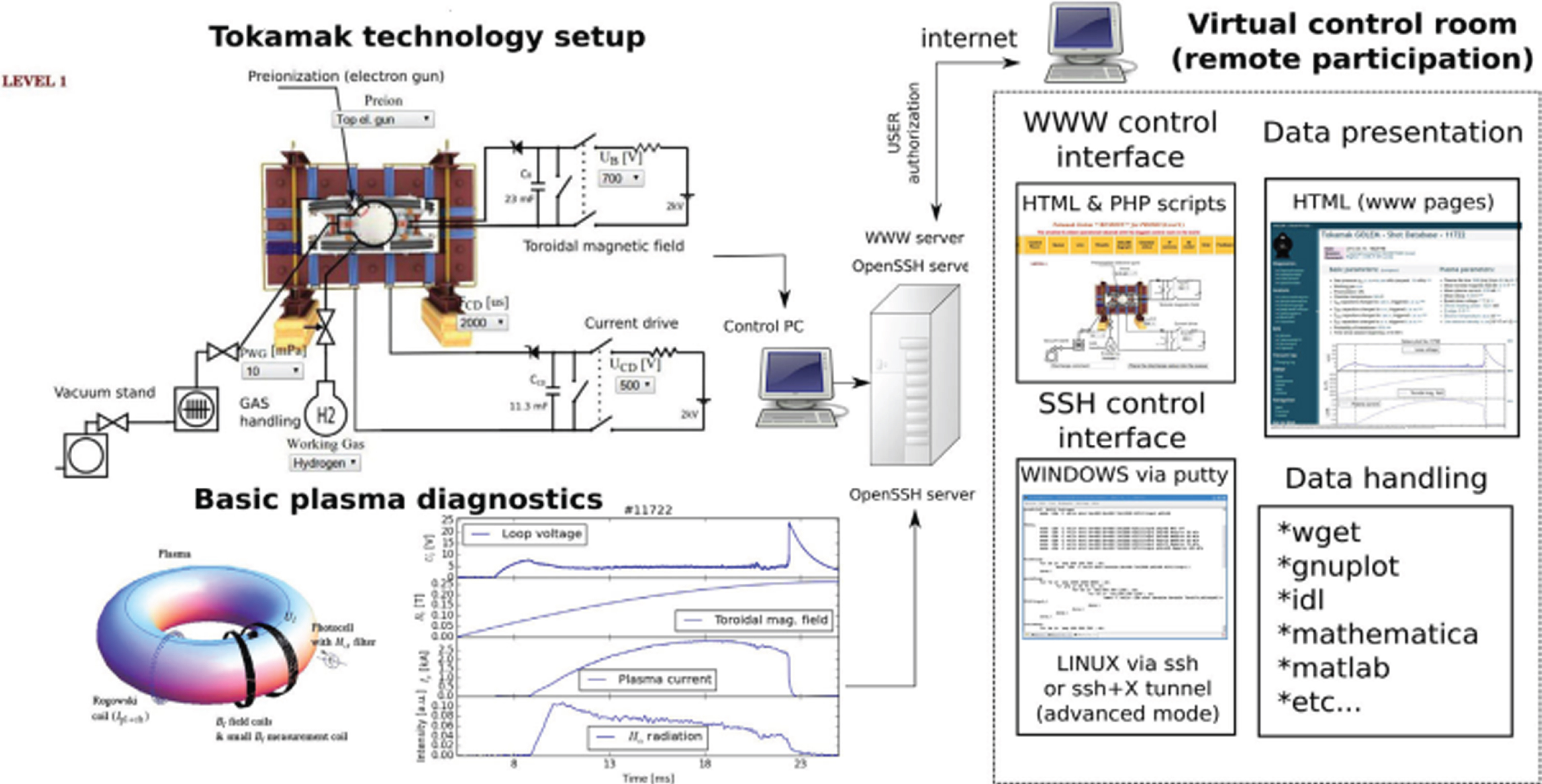
Schematic Representation [38] of GOLEM Tokamak Experimenter.

Table 1

Signals in GOLEM tokamak

S. No	Signal description	Acronym	Units
1	Total Input Power	P _total	W
2	Plasma Current	I _plasma	A
3	Plasma Density	Dens	m ^-3
4	Line Integrated Density	L _Dens	m ^-2
5	Safety Factor q₉₅	q ₉₅	s ^-1
6	Greenwald Density	ne _Greenwald	D
7	Toroidal Magnetic Field	B _t	T
8	Vertical Plasma Position	PVP	Z _m
9	Total Radiated Power	RAD	W

3.2 Ensemble learners

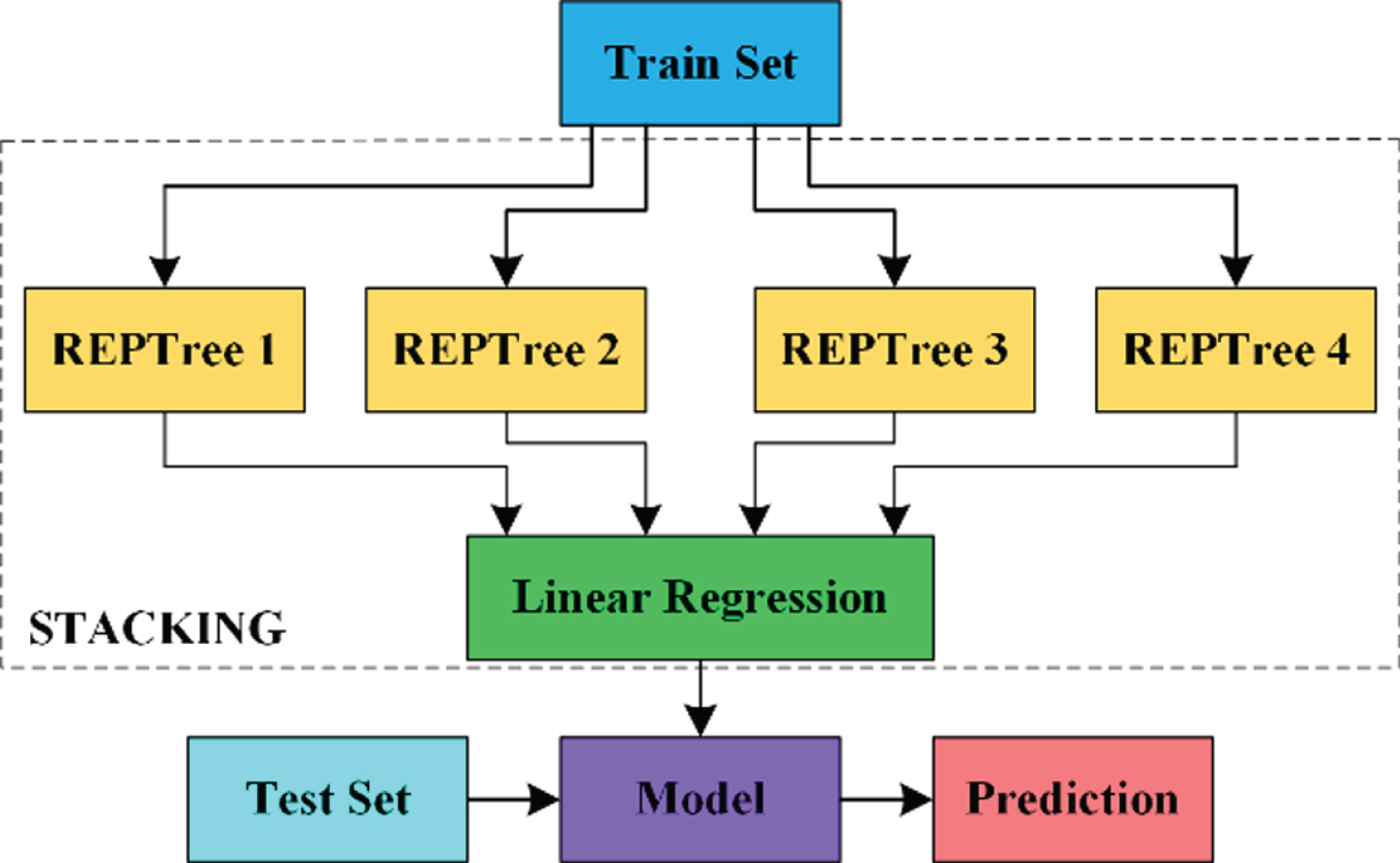
Figure 2 shows the working flow of the developed ensemble model. Out of the 187 shots, 132 shots consisting of 82 normal and 50 disruptive shots are used for training. Different values for CV folds, seed for randomizing the data, batch size and the portion of data required for pruning are used for the four base learners. Diversification among the base learners is achieved by selecting different hyperparameter values. The class distribution probability from each of the base learners forms the input to the meta-learners. The base learners with pruned REPTree does not overfit due to the use of CV. The meta-leaner model renormalizes the class probabilities and avoids the overfitting. The validation of the resulting model is performed on the unseen data. The test data or unseen data contains 55 shots that include 35 normal and 20 disruptive shots. The performance of the stacking model on the test data provides the generalized performance of the model.

Fig.2

Ensemble learning – Stacking.

3.2.1 Stacking

Table 2 depicts the Stacking algorithm. The function of stacking or blending is to combine predictions of base learners or original classifiers (level-0 models) using a meta learner (level-1 models), which provides the final prediction. The base learners can be the same algorithms or different algorithms or a combination of both. The outputs from the base learners are not a single class prediction but a probability estimate of each class. User-defined CV is performed by the base learners on the training data. The class probability distributions, which conveys both the prediction information and the confidence of classes are given as input to meta-learner. Irrespective of the base learner, Ting and Witten [39] introduced MLR as the level-1 classifier. The MLR discovers a linear function for every class by predicting the degree of confidence in class membership. After normalization, the expected degree of confidence is decoded as a class probability. The stacking method [40] used in this work employs MLR proposed in [33] and differs from the conventional stacking introduced by Wolpert [41]. The traditional stacking utilizes all the class probabilities from the base learners, while the variant of stacking used in this work utilizes only the class probabilities that are of interest. In our case, the class in focus is the disruptions in the Tokamak. The change is relevant even for two-class problems. Since the sum of all class probability distribution equals one, from the probability of one class (disruption), the probability of the other class (normal) is easily calculated. Specifics of the output from the base and meta learners is described in section 3.2.3. The modified stacking helps in faster training due to the reduced dimensionality input to the meta classifier.

Table 2
Algorithm for Stacking

Input: Training data J = { y_n, x_m } ; n = 0, 1

Output: Stacking model - M¹

1. Define the level-0 model on J

2. Set hyperparameters: k-fold (CV), size of pruning data, batch size, a seed for randomization

3. Repeat step 2 for the other three level-0 learners with different values

4. Execute base models with k-fold CV

5. $m_{1}^{0} = REPTree 1 (x)$

6. $m_{2}^{0} = REPTree 2 (x)$

7. $m_{3}^{0} = REPTree 3 (x)$

8. $m_{4}^{0} = REPTree 4 (x)$

9. Level-0 class probability output models for class i (0): P_ri (x) ; r = 1 -4

10. Level-0 class probability output models for class i′ (1): P_ri′ (x) =1 - P_ri (x)

11. Define level-1 model on P_ri, P_ri′

12. Stacking model output:

$M_{i}^{1} = {y_{0}, P_{ri} (x)}; class 0$ $M_{i^{'}}^{1} = 1 - {y_{0}, P_{ri} (x)}; class 1$

Input: Training data J = { y_n, x_m } ; n = 0, 1
1. Define the level-0 model on J
2. Set hyperparameters: k-fold (CV), size of pruning data, batch size, a seed for randomization
3. Repeat step 2 for the other three level-0 learners with different values
4. Execute base models with k-fold CV
5. $m_{1}^{0} = REPTree 1 (x)$
6. $m_{2}^{0} = REPTree 2 (x)$
7. $m_{3}^{0} = REPTree 3 (x)$
8. $m_{4}^{0} = REPTree 4 (x)$
9. Level-0 class probability output models for class i (0): P_ri (x) ; r = 1 -4
10. Level-0 class probability output models for class i′ (1): P_ri′ (x) =1 - P_ri (x)
11. Define level-1 model on P_ri, P_ri′
12. Stacking model output:
$M_{i}^{1} = {y_{0}, P_{ri} (x)}; class 0$ $M_{i^{'}}^{1} = 1 - {y_{0}, P_{ri} (x)}; class 1$

3.2.2 Base-classifier: REPTree

Figure 3 depicts a part of the generated REPTree, which mentions the split criterion for the attributes, entropy value, number of instances of an attribute at the nodes, the normal and disruptive class distribution.

Fig.3

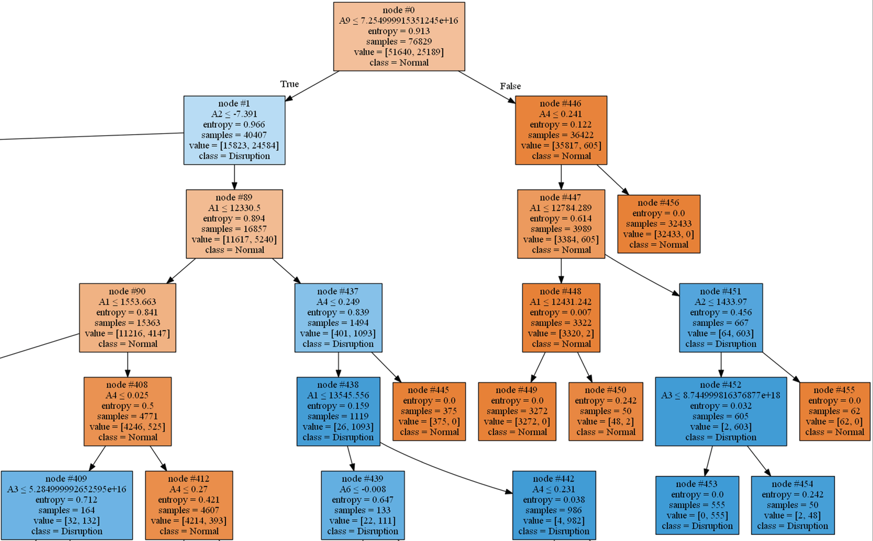
Part of Graphical Depiction of Tree in Stacking Ensemble Classifier.

The functioning of REPTree is the same as the C4.5 algorithm [42] in building a decision or regression tree, and they differ from C4.5 in the way pruning is done. Like C4.5, REPTree builds tree utilizing the information gain or variance reduction and handles the missing values by dividing instances into parts. REPTree algorithm sorts the numerical attributes only once. Other variable parameters are the minimum total weight of instances per leaf, maximum depth of the tree, and the size of folds used for pruning.

3.2.2.1. Gain criteria for tree generation. If X is the set of instances then the number of instances in X that belong to the class y_i is denoted as freq (y_i, X). The number of instances is represented by |X|. The probability of selecting one example from a set of X instances and declaring that it belongs to y_i (classifromoutputy) is given by $p_{i} = \frac{freq (y_{i}, X)}{| X |}$ (1) (where i = 0 and 1 for two class and i = 0 to m for multiclass). The information conveyed in bits is $- \log_{2} (\frac{freq (y_{i}, X)}{| X |})$ (2)

The information to a class member is given by summing the classes in proportion to the frequencies as

$\begin{matrix} Info (x) = - \sum_{i = 1}^{m} \frac{freq (y_{i}, X)}{| X |} \\ * {log}_{2} (\frac{freq (y_{i}, X)}{| X |}) bits \end{matrix}$ (3)Info (x) is the average amount of information in bits required to determine the class of an example in X.

After X is split to k subsets on attribute A, the expected information is the weighted sum over the subsets and is represented as $Split Info (T) = \sum_{j = 1}^{k} \frac{| X_{i} |}{| X |} * {log}_{2} (\frac{| X_{i} |}{| X |})$ (4)

The information gained by partitioning X with attribute A is $Gain (A) = Info (x) - {Info}_{T} (x)$ (5)

As entropy increases, the information gain decreases and vice versa. The split occurs where the information gain is high, which is equivalent to a high reduction in entropy.

The gain criterion which helps classification is $Gain ratio (A) = \frac{Gain (A)}{Split info (A)}$ (6)

If the split is trivial, split information is less, and the gain criterion is unstable, which is avoided by selecting attribute A to maximize the gain ratio whereas the information gain should be significant. Equation 3 can be written as $Entropy (T) orH (T) = - \sum_{i = 1}^{m} p_{i} * {log}_{2} p_{i}$ (7)

For binary classification, entropy is minimum when all the instances belong to the same class and maximum when either class is 50% or 0.5 $\begin{matrix} Entropy = - 0.5 * \log_{2} (0.5) - 0.5 * \log_{2} (0.5) = 1 \end{matrix}$

If n_c, d_c and t_c represent the normal, disruption and total count in the Golem dataset; the entropy is $\begin{matrix} H (T) = & - \frac{n_{c}}{t_{c}} * \log_{2} (\frac{n_{c}}{t_{c}}) - \frac{d_{c}}{t_{c}} * \log_{2} (\frac{d_{c}}{t_{c}}) ≅ \\ - 0.328 * \log_{2} (0.328) - 0.672 \\ * \log_{2} (0.672) ≅ 0.913 \end{matrix}$

The average information required to encode the class label for a random instance from the dataset is around 1 bit.

All the attributes in the Golem dataset are continuous. The steps to find the threshold t that maximize the splitting criterion are

The instances in X are sorted according to their values as v1, v2, v3 … . vn

Each pair of adjacent values form a valid threshold vi + (vi + 1)/2 and a corresponding partition.

The threshold with the best value of splitting criterion is chosen as the split point.

For an attribute say A1, the information gain is given as $Info gain (T, A 1) = H (T) - H (T | A 1)$ (8)

Let us consider the split for attribute A1. Let the left and right split from attribute A1 be represented as L (node 90) and R (node 437). Each node indicates the distribution of the instances for normal and disruption class. The instances or count at node 90 is denoted as [n_lc, d_lc] and node 437 as [n_rc, d_rc]. The total count at node 90 is denoted as t_lc and node 437 as t_rc respectively. Let T_c = t_lc + t_rc. From Fig. 3, $\begin{matrix} [n_{lc}, d_{lc}] = [11216, 4147] \\ [n_{rc}, d_{rc}] = [401, 1093] \\ t_{lc} = 11216 + 4147 = 15363 \\ t_{rc} = 401 + 1093 = 1494 \\ T_{c} = 16857 \end{matrix}$

As indicated in node 89 of Fig. 3, for attribute A1, $H (T) = 0.894$

The entropy at node 90 (L) is calculated as $\begin{matrix} H (L) = - \frac{n_{lc}}{t_{lc}} * \log_{2} (\frac{n_{lc}}{t_{lc}}) - \frac{d_{lc}}{t_{lc}} * \log_{2} (\frac{d_{lc}}{t_{lc}}) \\ ≅ - 0.730 * \log_{2} (0.730) - \\ 0.270 * \log_{2} (0.270) \\ ≅ 0.841 bits \end{matrix}$

Similarly, the entropy at node 437 (R) is given by $\begin{matrix} H (R) = - \frac{n_{rc}}{t_{rc}} * \log_{2} (\frac{n_{rc}}{t_{rc}}) - \frac{d_{rc}}{t_{rc}} * \log_{2} (\frac{d_{rc}}{t_{rc}}) \\ ≅ - 0.268 * \log_{2} (0.268) - \\ 0.731 * \log_{2} (0.731) \\ ≅ 0.839 bits \end{matrix}$

Information after including attribute A1 is $\begin{matrix} H (T | A 1) = \frac{t_{lc}}{T_{c}} * H (L) + \frac{t_{rc}}{T_{c}} * H (R) \\ ≅ 0.911 * 0.841 + 0.89 * 0.841 \\ ≅ 0.8411 bits \end{matrix}$

From equation 8, info gain is $\begin{matrix} Info gain (T, A 1) = 0.894 - 0.842 \\ ≅ 0.0529 bits \end{matrix}$

Table 3 lists the entropy calculation for six values of attribute A1 and their corresponding information gain.

Table 3

Entropy and Information Gain for Attribute A1

Attribute A1				Entropy		Info
≤12180.5		>12180.5				Gain
n _lc	d _lc	n _rc	d _rc	H (L)	H (R)
11198	4136	419	1103	0.841	0.848	0.0523
≤12230.5		>12230.5
n _lc	d _lc	n _rc	d _rc	H (L)	H (R)
11202	4137	415	1102	0.841	0.846	0.0525
≤12280.5		>12280.5
n _lc	d _lc	n _rc	d _rc	H (L)	H (R)
11208	4141	409	1098	0.841	0.843	0.0527
≤ 12330.5		>12330.5
n _lc	d _lc	n _rc	d _rc	H (L)	H (R)
11216	4147	401	1093	0.841	0.839	0.0529
≤12380.5		>12380.5
n _lc	d _lc	n _rc	d _rc	H (L)	H (R)
11219	4154	398	1085	0.842	0.837	0.0525
≤12430.5		>12430.5
n _lc	d _lc	n _rc	d _rc	H (L)	H (R)
11225	4163	392	1076	0.843	0.839	0.0523

The split occurs at attribute A1 for the value where the information gain in maximum (0.0529).

3.2.2.2. Pruning. Decision trees follow a greedy approach to generate the tree. The splits on the nodes continue until there is information gain, which leads to deep trees. Overfitting occurs due to the depth of trees resulting in weak performance on test data. The process of replacing subtrees with simpler subtrees or leaf nodes with little effect on classification accuracy is called pruning. The difference in the accuracy of the unpruned and pruned trees should be negligible. Pruning avoids complex model and overfitting.

The difference between C4.5 and REPTree algorithms is that C4.5 a pessimistic approach for pruning and REPTree utilize reduced error pruning. In REPTree, the training dataset is divided into two, namely growth and pruning dataset. The first tree is generated on the growth dataset. Pruning dataset is used to minimize the error from the growth tree by adopting the bottom-to-top approach. The growth and pruning datasets are re-split at each cycle of the algorithm. The splitting enables covering all instances of the training data by both the datasets. When the next split in the dataset is used, each parent examines the error of the child nodes. If the error of the parent node is greater than the child node, then the child nodes are removed. The challenge is using REPTree is that a large training data is needed for training, and the criteria should be different for creating the growth and pruning datasets. C4.5 algorithm before reduced error pruning produced 527 nodes and 264 leaves and after pruning generated 369 nodes and 185 leaves. There is a reduction of about 30% in the number of nodes and leaves after pruning.

3.2.2.3. Splitting and stopping criteria. For numerical attributes, binary splits are produced, and for categorical attributes, k - way splits are produced. The numerical attributes are sorted, and each value is considered as split points. The stopping criteria is a minimum of two children per leaf. Only splits where information gain values are better than average value is considered for a split to mitigate highly imbalanced data partitioning.

3.2.2.4. Computational complexity. For a tree with n instances and m attributes, the standard depth of the tree with n leaves is given by $O (log n) .$ (9)

With m attributes, at each tree depth, the whole set of n instances need to be taken into account. For log n depths within the tree, the volume of work for one attribute is $O (n log n)$ (10)

All the attributes are considered at each node, and hence the complexity of building the trees are O (mn log n). The numeric attributes must be sorted only once, and with an appropriate algorithm, the initial sort requires O (n log n) for each of the m attributes. For pruning, through subtree replacement, an error estimate at every tree node is made with the tree having a maximum of n leaves. For a binary tree, with a numeric attribute, there would be 2n - 1 nodes. The subtree replacement complexity is $O (n)$ (11)

Lastly, the complexity of subtree lifting must be considered. At worst, each instance is reclassified at every node, and it’s a two-step operation with one being performed at the root with O (log n) and one of average depth is $O \frac{(log n)}{2}$ . The complexity of subtree lifting is $O (n (log n^{2})$ (12)

Combining all the operations, the total complexity of the C4.5 algorithm is $O (mn log n) + O (n (log n^{2})$ (13)

3.2.3 Meta-classifier – Multi-response Linear Regression (MLR)

Linear regression is used to find the relationship between input and output and is widely applied in statistics and in machine learning is suitable only for regression problems. MLR is derived from the linear regression algorithm with least-squares. A dataset having real-values as attributes intended for classification can be adapted as an MLR task. y₀, y₁ are the individual classes for the classification task. If y₀ or y₁ equals zero in a classification task; the corresponding linear value in regression is also zero. Likewise, regression value is one the if y₀ or y₁ equals one.

Let J denote the dataset with $J = {y_{n,} x_{m}}$ (14) wherein y_n are the classes and x_m are the number of input instances. For binary classification n = 2. The models obtained on the training data from the base learners are represented as $m_{r}^{0}$ where k are the number of base learners and ‘0’ specifies level-0 models.

For the REPTree algorithm, let l_i denote the number of instances from the training data with class i at leaf l. Let us assume i an i′ denote class 0 and 1 respectively, then by Laplace transform, probability of class i (0) is, $P_{i} (x) = 1 - \frac{l_{i} + l_{i^{'}} + 1}{l_{i} + l_{i^{'}} + 2}$ (15)

The probability of other class i′ (1) is, $P_{i^{'}} (x) = 1 - P_{i} (x)$ (16)

If i denote the class, the probability of i^th class output on training instances x of the base learners is given as P_ri (x). In our case, i = 2 (0 and 1) and r = 1, 2, … R. When one class probability is produced, the likelihood of another class is easily derived. Hence, minority class (0) probabilities from all the base learners (R = 4) are denoted as $P_{10} (x), P_{20} (x), P_{30} (x), P_{40} (x)$ (17)

The final model with y₀ as output is given by $M_{i}^{1} = {y_{0}, P_{10} (x), P_{20} (x), P_{30} (x), P_{40} (x)}$ (18) and the linear regression for class i is given by ${LR}_{i} = \sum_{r}^{R} α_{ri} (x) P_{ri} (x)$ (19)α are the coefficients of attributes learned by the model.

4 Results and discussion

Table 4 presents a comparison of the widely used machine learning algorithms along with ensemble classifiers like bagging, boosting, and voting for the GOLEM Tokamak. The investigation was conducted on the Tokamak dataset with training – testing split of 70%–30% thereby experimenting 132 for training and 55 for testing. In general, tree algorithms performed better than the probabilistic models such as Bayes Net and Naive Bayes. Among the ensemble models, voting registered the least score. CART as the decision tree gave the best result for both Bagging and Boosting (AdaBoostM1, Gradient Boosting) techniques. The performance of Random Forest decreased due to the recall metric.

Table 4
Comparative results for different algorithms

Algorithms A P R F1

CART 89.613 0.950 0.836 0.890

C4.5 90.093 0.957 0.839 0.894

REPTree 90.246 0.959 0.841 0.896

Logistics regression 72.282 0.653 0.953 0.775

LDA 85.722 0.710 0.844 0.808

Bayes Net 75.768 0.800 0.738 0.767

Naïve Bayes 72.563 0.656 0.948 0.776

KNN 84.435 0.687 0.742 0.770

AdaBoostM1 89.916 0.949 0.843 0.893

Gradient Boosting 88.430 0.755 0.977 0.860

Voting 84.978 0.904 0.783 0.839

Bagging 90.829 0.982 0.831 0.901

Random Forest 93.803 1.00 0.876 0.934

Stacking 97.320 0.973 0.973 0.973

Algorithms	A	P	R	F1
CART	89.613	0.950	0.836	0.890
C4.5	90.093	0.957	0.839	0.894
REPTree	90.246	0.959	0.841	0.896
Logistics regression	72.282	0.653	0.953	0.775
LDA	85.722	0.710	0.844	0.808
Bayes Net	75.768	0.800	0.738	0.767
Naïve Bayes	72.563	0.656	0.948	0.776
KNN	84.435	0.687	0.742	0.770
AdaBoostM1	89.916	0.949	0.843	0.893
Gradient Boosting	88.430	0.755	0.977	0.860
Voting	84.978	0.904	0.783	0.839
Bagging	90.829	0.982	0.831	0.901
Random Forest	93.803	1.00	0.876	0.934
Stacking	97.320	0.973	0.973	0.973

4.1 Accuracy (A)

The number of instances identified correctly. $Accuracy = \frac{TP + TN}{TP + TN + FP + FN}$

4.2 Precision (P)

The ratio of correct disruptions to the total instances classified as disruptions by the model. $Positive Predict Rate / Precision = \frac{TP}{TP + FP}$

4.3 Recall (R)

The ratio of correct disruptions to instances that belong to the disruption class in the dataset. $Recall = \frac{TP}{TP + FN}$

4.4 F1 Score

Defines the trade-off between precision and recall through a harmonic mean of precision and recall. $F 1 Score = \frac{2 \times P \times R}{P + R}$

4.5 False positive rate

The ratio of normal instances classified as disruptions to the total number of normal instances. $False Positive Rate = \frac{FP}{TN + FP}$

4.6 ROC and precision-recall curve

Figure 4 shows the ROC curve of the developed ensemble model for both normal and disruptive shots.

The trade-offs between False Positive Rate (X-axis) and True Positive Rate (Y-axis) summarizes the predictive performance of the ensemble learners. The ROC curve separates the error cost calculations from the performance of the ensemble learners and is invariable under dynamic class distributions.

Fig.4

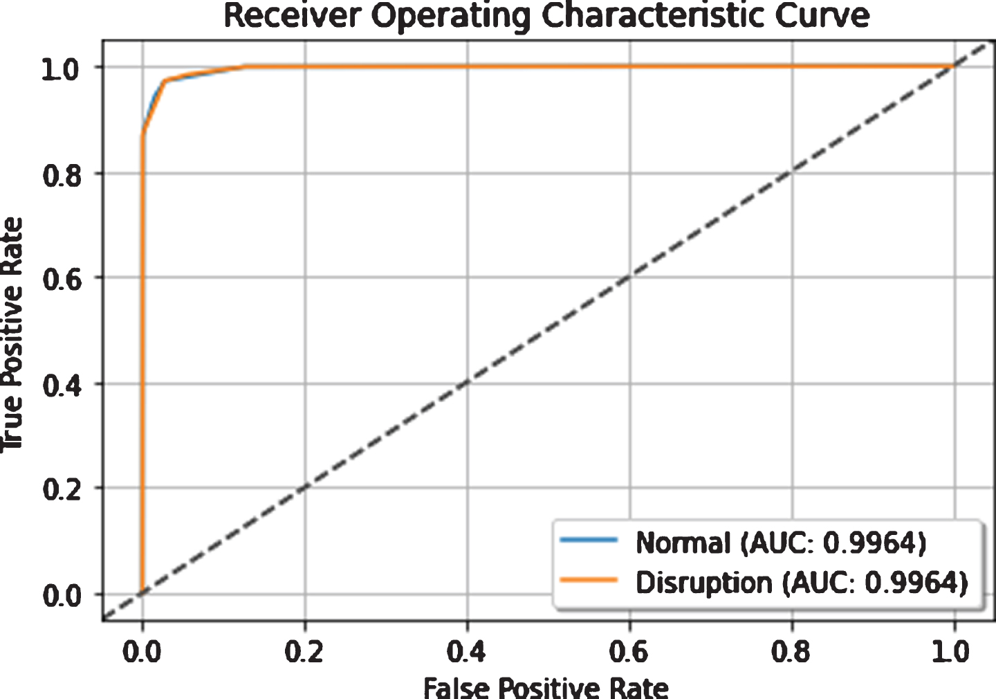
ROC curve of the stacking model.

Figure 5 shows the Precision-Recall (PR) curve for both normal and disruptive shots. PR is a useful diagnostic method for binary classification when the class distribution is imbalanced. It is a plot with Recall (X-axis) and Precision (Y-Axis).

Fig.5

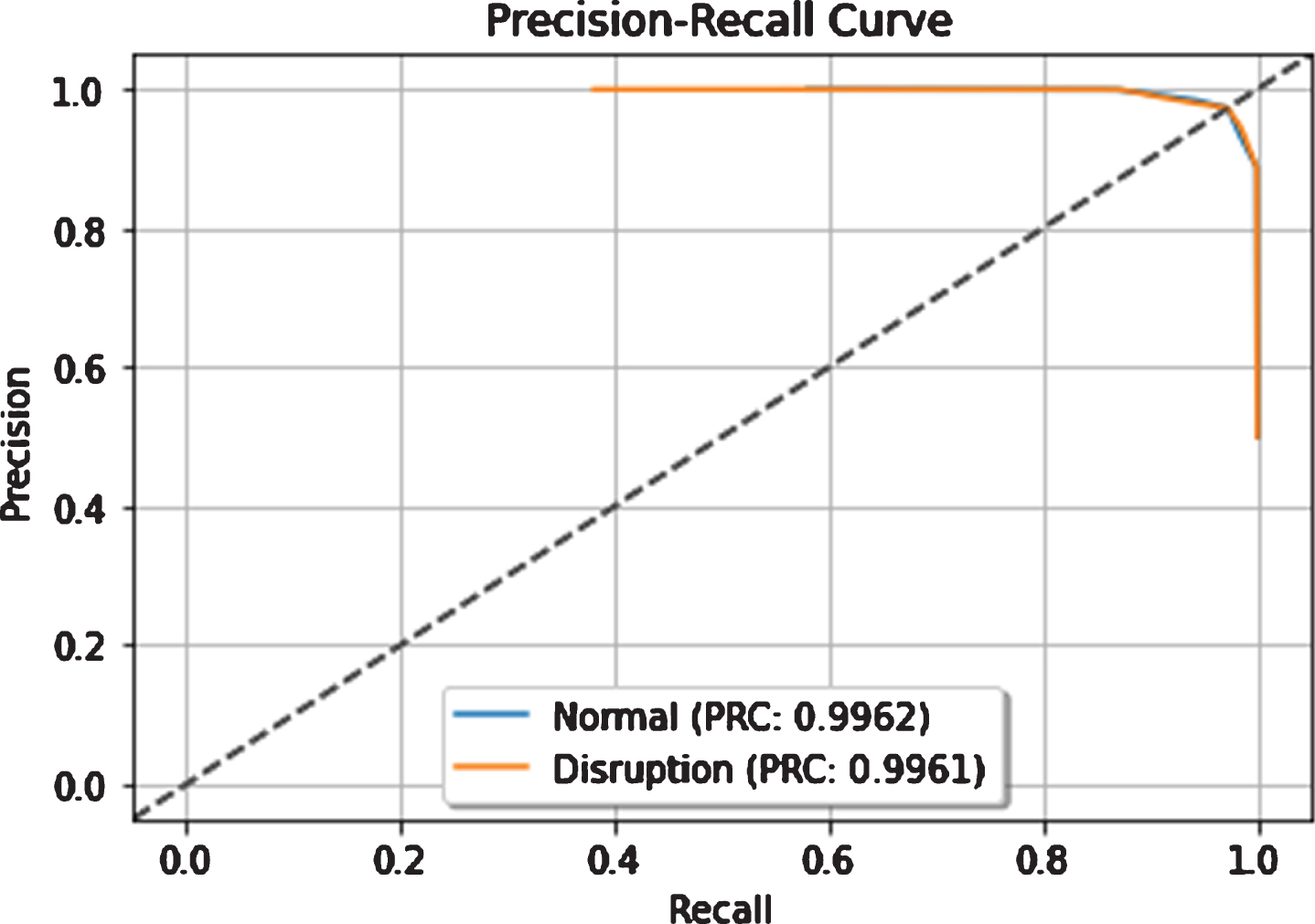
Precision-recall curve of the stacking model.

5 Conclusion and future works

Disruptions in a Tokamak system must be detected at the earliest to avoid significant damage to the components and the vessel. There has been substantial literature in disruption prediction with machine learning and ensemble methods. Our implementation of stacking has reduced complexity and faster training than other ensemble methods. The short decision trees resulted in a reduction in tee size of about 33% from the regular trees both with nodes and leaves. Further, MLR, which is employed mainly in regression, is exercised as meta-learner for classification. The stability of our model is substantiated with its minor accuracy variation over its thirty iterations of train and test. A comparative study comprising decisive metrics executed over the standard train-test split of the dataset is demonstrated with often used algorithms. Stacking prevailed over other algorithms in terms of quantitative results. However, it must be noted that the stacking is implemented on the GOLEM Tokamak dataset. Performance of stacking might vary with other datasets and may not generalize to other applications.

Probable future works are a) experimenting a stacking ensemble classifier in a real-time environment and datasets from other domain b) to implement neural networks with more data c) operate on raw sensor data and provide an end-to-end solution through deep learning techniques d) exploring the transformation of the dataset to a time-series forecasting problem e) determining effective ways to give feedback to the plasma control system.

References

Sengupta

, Ranjan

, Forecasting disruptions in the ADITYA tokamak using neural networks, Nuclear Fusion 40(12) (2000), 1993–2008.

Sengupta

, Ranjan

, Prediction of density limit disruption boundaries from diagnostic signals using neural networks, Nuclear Fusion 41(5) (2001), 487–501.

Sengupta

, Ranjan

, Identification of plasma parameters and optimization of magnetic sensors in the Superconducting Steady-State Tokamak-1 using neural networks, Fusion Technology 39(1) (2001), 1–17.

Windsor

C.G.

, Pautasso

, Tichmann

, Buttery

R.J.

, Hender

T.C.

, A cross-tokamak neural network disruption predictor for the JET and ASDEX Upgrade tokamaks, Nuclear Fusion 45(5) (2005), 337–350.

Pautasso

, et al., On-line Prediction and mitigation of disruptions in ASDEX Upgrade, Nuclear Fusion 290–293(1) (2002), 100–108.

Rea

, Granetz

R.S.

, Montes

, Tinguely

R.A.

, Eidietis

, Hanson

J.M.

, Sammuli

, Disruption prediction investigations using Machine Learning tools on DIII-D and Alcator C-Mod, Plasma Physics and Controlled Fusion 60(8) (2018), 1–13.

Granetz

R.S.

, Rea

, Montes

K.J.

, Tinguely

R.A.

, Eidietis

, Meneghini

O.M.

, Chen

D.L.

, Shen

, Xiao

B.J.

, Machine Learning for Disruption Warning on Alcator C-Mod, DIII-D, and East Tokamas, Nuclear Fusion 59(9) (2019), 1–8.

Rea

, Montes

K.J.

, Erickson

K.G.

, Granetz

R.S.

, Tinguely

R.A.

, A real-time machine learning-based disruption predictor in DIII-D, Nuclear Fusion 59(9) (2019), 1–10.

Cannas

, Fanni

, Marongiu

, Sonato

, Disruption forecasting at JET using neural networks, Nuclear Fusion 44(1) (2004), 68–76.

10.

Yoshino

, Neural-net predictor for beta limit disruptions in JT-60U, Nuclear Fusion 45(11) (2005), 1232–1246.

11.

Yoshino

, Neural-net disruption predictor in JT-60U, Nuclear Fusion 43(12) (2003), 1771–1786.

12.

M.Z. , G.Z. , Wang

S.Y.

, Chen

Z.Y.

, Huang

D.W.

, Tong

R.H.

, Yan

, Wei

Y.N.

and Ma

T.K.

, Prediction of density limit disruptions on the J-TEXT tokamak, Plasma Physics and Controlled Fusion 58(5) (2016), 1–10.

13.

Gerhardt

S.P.

, Darrow

D.S.

, Bell

R.E.

, Leblanc

B.P.

, Menard

J.E.

, Mueller

, Roquemore

A.L.

, Sabbagh

S.A.

, Yuh

, Detection of disruptions in the high-β spherical torus NSTX, Nuclear Fusion 53(6) (2013), 1–19.

14.

Zakharov

L.E.

, Galkin

S.A.

, Gerasimov

S.N.

, Understanding disruptions in tokamaks, Physics of Plasmas 19(5) (2012).

15.

Boozer

A.H.

, Theory of tokamak disruptions, Physics of Plasmas 19(5) (2012).

16.

Quinlan

J.R.

, Simplifying Decision Trees, International Journal of Man-Machine Studies 27(3) (1987), 221–234.

17.

Ting

K.M.

, Witten

, Issues in Stacked Generalization, Journal of Artificial Intelligence Research 10 (1999), 271–289.

18.

GOLAM Tokamak. http://golem.fjfi.cvut.cz/.

19.

Sengupta

, Ranjan

, Modified neural networks for rapid recovery of tokamak plasma parameters for real time control, Review of Scientific Instruments 73(7) (2002), 2566–2577.

20.

Wroblewski

, Jahns

G.L.

, Leuer

J.A.

, Tokamak Disruption Alarm Based On A Neural Network Model Of The High-Beta Limit, Nuclear Fusion 37(6) (1997), 725–741.

21.

Aledda

, Cannas

, Fanni

, Pau

, Sias

and the A.U. Team, Improvements in disruption prediction at ASDEX Upgrade, Fusion Engineering and Design 96–97 (2015), 698–702.

22.

Cannas

, Fanni

, Pautasso

, Sias

, Sonato

, An adaptive real-time disruption predictor for ASDEX upgrade, Nuclear Fusion 50(7) (2010).

23.

Cannas

, Fanni

, Pautasso

, Sias

, Disruption prediction with adaptive neural networks for ASDEX Upgrade, Fusion Engineering and Design 86(6–8) (2011), 1039–1044.

24.

Rattá

G.A.

, Vega

and Murari

, Improved feature selection based on genetic algorithms for real time disruption prediction on JET, Fusion Engineering and Design 87(9) (2012), 1670–1678.

25.

Murari

, Lungaroni

, Peluso

, Gaudio

, Vega

, Dormido-Canto

, Baruzzo

M.M.

, Gelfusa

, Contributors

, Adaptive predictors based on probabilistic SVM for real time disruption mitigation on JET, Nuclear Fusion 58(5) (2018), 1–31.

26.

Vega

, Murari

, Dormido-Canto

, Moreno

, Pereira

, Acero

, Adaptive high learning rate probabilistic disruption predictors from scratch for the next generation of tokamaks, Nuclear Fusion 54(12) (2014), 1–17.

27.

Murari

, Lungaroni

, Gelfusa

, Peluso

, Vega

, Adaptive learning for disruption prediction in non-stationary conditions, Nuclear Fusion 59(8) (2019).

28.

Yokoyama

, Miyoshi

, Hiwatari

, Isayama

, Matsunaga

, Oyama

, Igarashi

, Okada

, Ogawa

, Prediction of high-beta disruptions in JT-60U based on sparse modeling using exhaustive search, Fusion Engineering and Design 140 (2019), 67–80.

29.

Tinguely

R.A.

, Montes

K.J.

, Rea

, Sweeney

, Granetz

R.S.

, An application of survival analysis to disruption prediction via Random Forests, Plasma Physics and Controlled Fusion 61(9) (2019), 1–24.

30.

Rea

, Granetz

R.S.

, Exploratory machine learning studies for disruption prediction using large databases on DIII-D, Fusion Science and Technology 74(1–2) (2018), 89–100.

31.

Murari

, Rossi

, Peluso

, Lungaroni

, Gaudio

, Gelfusa

, Ratta

, Vega

, Contributors

, On the transfer of adaptive predictors between different devices for both mitigation and prevention of disruptions, Nuclear Fusion, (In Press), 2020.

32.

Czarnowski

, Jędrzejowicz

, Learning from examples with data reduction and stacked generalization, Journal of Intelligent and Fuzzy Systems 32(2) (2017), 1401–1411.

33.

Shi

, Liu

, Li

, Prediction of pipe performance with stacking ensemble learning based approaches, Journal of Intelligent and Fuzzy Systems 34(6) (2018), 3845–3855.

34.

Jain

, Alzubi

J.A.

, Jain

, Joshi

, Assessing risk in life insurance using ensemble learning, Journal of Intelligent and Fuzzy Systems 37(2) (2019), 2969–2980.

35.

Svoboda

, Huang

, Mlynáč

, Pokol

G.I.

, Stöckel

and Vondrášek

, Multi-mode remote participation on the GOLEM tokamak, Fusion Engineering and Design 86 (2011), 1310–1314.

36.

Svoboda

, Dvornova

, Dejarnac

, Prochazka

, Zaprianov

, Akhmethanov

, Bogdanova

, Remote operation of the GOLEM tokamak with hydrogen and helium plasmas, Journal of Physics: Conference Series 768(1) (2016).

37.

Grover

, Kocman

, Odstrcil

, Matusu

, Stöckel

, Svoboda

, Vondrasek

, Zara

, Remote operation of the GOLEM tokamak for Fusion Education, Fusion Engineering and Design 112 (2016), 1038–1044.

38.

Kramer

, Khoury

H.J.

, Ferrari

, Gualdrini

, Huh

, Bolch

W.E.

, Demarco

J.J.

, Cagnon

C.H.

, Remote operation of the GOLEM tokamak with hydrogen and helium plasmas, 2000.

39.

Ting

K.M.

, Witten

I.H.

, Issues in Stacked Generalization, 10 (1999), 271–289.

40.

Seewald

A.K.

, How to Make Stacking Better and Faster While Also Taking Care of an Unknown Weakness, 2002.

41.

Wolpert

D.H.

, Stacked generalization, Neural Networks 5(2) (1992), 241–259.

42.

Quinlan

J.R.

, C4.5: Programs for Machine Learning, Morgan Kaufmann 5(3) (1993), 1–302.