A fuzzy based high-resolution multi-view deep CNN for breast cancer diagnosis through SVM classifier on visual analysis

Abstract

Breast cancer should be diagnosed as early as possible. A new approach of the diagnosis using deep learning for breast cancer and the particular process using segmentation strategies presented in this article. Medical imagery is an essential tool used for both diagnosis and treatment in many fields of medical applications. But, it takes specially trained medical specialists to read medical images and make diagnoses or treatment decisions. New practices of interpreting medical images are labour exhaustive, time-wasting, expensive, and prone to error. Using a computer-aided program which can render diagnosis and treatment decisions automatically would be more beneficial. A new computer-based detection method for the classification between compassionate and malignant mass tumours in mammography images of the breast proposed. (a) We planned to determine how to use the challenging definition, which produces severe examples that boost the segmentation of mammograms. (b) Employing well designing multi-instance learning through deep learning, we validated employing inadequately labelled data of breast cancer diagnosis using a mammogram. (c) The study is going through the Deep Lung method incorporating deep multi-dimensional automated identification and classification of the lung nodule. (d) By combining a probabilistic graphic model in deep learning, it authorizes how weakly labelled data can be used to improve the existing breast cancer identification method. This automated system involves manually defining the Region Of Interest (ROI), with the region and threshold values based on the next region. The High-Resolution Multi-View Deep Convolutional Neural Network (HRMP-DCNN) mainly developed for the extraction of function. The findings collected through the subsequent in available public databases like mammography screening information database and DDSM Curated Breast Imaging Subset. Ultimately, we’ll show the VGG that’s thousands of times quicker, and it is more reliable than earlier programmed anatomy segmentation.

Keywords

Deep convolutional neural network computer-based automated detection breast cancer screening deep learning machine learning mammography fuzzy logic.

1 Introduction

Breast cancer is ubiquitous as one of the critical bases of feminine mortality. The volume of cancer cases predicted for 2025, and it will cross over 19.3 million cases World Health Organization (WHO) conferred. Recently, the majority of the countries moving towards a common area of research about breast cancer occur with women [1]. Breast cancer mortality rates are also high, reflecting about 20% of cancer-related deaths. Accurately the earlier detection along with the evaluation of breast cancer is critical while raising the mortality rate. Magnetic Resonance Imaging (MRI) is the supreme most effective unconventional to mammograms. To date, mammography played as the most valuable tool for screening the general population.

Nevertheless, the exact identification and analysis of a breast lesion based merely on mammography results are challenging and hugely dependent on radiologist’s experience, resulting in a large number of inappropriate positives and additional tests. Overall, after a screening mammogram, the recall rate is between 10–15%. It refers to about 3.3 to 4.5 million call-back exams for further research. After an inconclusive mammogram, the enormous majority of the women requested to reappearance undergo an additional mammogram/ultrasound through confirmation. Most of these false-positive results represent natural breast tissue. It advised that only 10 to 20% of women who have an irregular screening mammogram undergo a biopsy [2]. Only 20–40% of these biopsies produce a cancer diagnosis.

Deep learning has, in recent years, been a successful and influential method for leading the Artificial Intelligence (AI) era [3]. Recently, deep learning has seen massive success in challenging issues like object recognition by automatic speech recognition, natural images, and machine translation [4]. This success has prompted an increase in interest in the application of profound convolutional networks to medical imaging. Several recent studies have shown the potential for such networks to be extended to medical imaging, including breast screening mammography; however, without exploring the fundamental differences between medical and natural images and their effect on the design choices and efficiency of the proposed model.

For example, several recent works either downscaled a whole picture significantly or concentrated on classifying a small region of interest. It could be detrimental to the output of such models given the well-known reliance on fine details of breast cancer screening, such as the presence of a cluster of microcalcification, as well as global structures, such as the symmetry between two breasts. On the other hand, with the breakthroughs, as mentioned earlier, from deep learning, self-driving car, personal assistant apps (Alexa, Google Home, etc.), AI for health-care are emerging problems. In this study, we concentrate on numerous topics as well as mammograms, computed pulmonary tomography images, deep learning for automated medical image analysis and head, and neck CT images that might help radiologists enhance the diagnosis [5].

In this research, in the sense of breast cancer screening, we investigated the study and understanding of the fundamental properties of deep convolutional networks. Work is attempting to lighten the burden throughout the two directions, as the ability to create in-depth learning-based segmentation and also a vital problem to analyze the medical image due to mass segmentation that generates the morphological characteristics which give strong evidence over mammogram diagnosis. Secondly, related to ground-truth identification or segmentation, Electronic Medical Report (EMR) can quickly obtain labels at the image-level. Using the picture level mark, we design a new paradigm for the diagnosis of breast cancer. The approach varies from traditional approaches that rely on Regions of interest (ROIs) that require considerable annotation determinations.

The results achieved were False Positive Rate (FPR) with 31% and True Positive Rate (TPR) with 90%. We used VGG to identify benign and malignant masses through DDSM dataset mammograms, and accuracy was 66%. We propose a motivating modification of HRMP-DCNN. There are two stages in producing output using Multi-View High-Resolution Deep Convolutional Neural Network. The more number of convolutional and pooling layers are added discretely to each one of the views during the first step. We started by building a large-scale data set of 201,698 mammographic screening exams (886,437 images) [6] obtained at multiple sites within our organization. We’ve created a novel DCN that can handle multiple views of mammography screening and use big, high-resolution images without downscaling. We analyzed the effect of the data set size and image resolution on the screening efficiency of the proposed HRMP-DCNN [7], which would serve as a de facto guideline to improve future profound neural networks for medical imaging. Lastly, we conducted a reader study, which showed that our model is almost as accurate on a random subset of the test set as a committee of radiologists with the same data presented. Besides, we found that we were obtaining the best results by averaging our model’s predictions with the radiologist’s committee predictions.

2 Related works

Deliberated [8] the possibility of using computational neural networks is to diagnose breast cancer accurately. The scholar compares statistical neural networks on the WBCD database to Multi-Layer Perceptron. For classification, they used General Regression Neural Network (GRNN), Probabilistic Neural Network (PNN), Radial Basis Function (RBF), with a complete performance of 96.18% in RBF, 97% in PNN, 98.8% in GRNN and 95.74% in MLP. Thus it is proven where the mathematical mechanisms of the neural network can be used to identify breast cancer.

In [9], endeavored to develop a neural network to diagnose breast cancer and Negative correlation training process was introduced for decomposing and to solve the problematic situation automatically. Right now creator talked about two methodologies, for example, developmental methodology and outfit approach, where transformative methodology can be utilized to naturally configuration smaller neural systems. The way to deal with the gathering planned for taking care of significant issues, yet it was proceeding.

The author has added 699 data, which have incomplete and deleted values, leaving 683 data. Two experimental designs performed using those values. The first experiment consisted of five 9-3-1 Multi-Layer Perception trials (i.e., 9 inputs, 3 hidden nodes, and 1 output node), and the next one that consist of 9-9-1 Multi-Layer Perception. After 400 generations, the outcome of the first experiment in every five hearings was 97.5% accuracy. In the second test, the best performance recorded for lesser hidden nodes with an accuracy rate of 98.2% compared to the previous experiment.

The report was submitted by [10] logistic regression compared with the artificial neural network. It related multi-layer perceptron Neural Networks (NNs) using Standard Logistic Regression (SLR), which classify significant covariates affecting disease-free survival (DFS), cancer-caused mortality, and breast cancer patient disease reappearance through area Under Receiver-Operating Characteristics (AUROC).

The Computer-Aided Diagnosis (CAD) [11] advances inaccuracy of interpreting called mammograms, as early as possible in detecting tumours and the differentiation in malignant ones and benign. For example, the presence of clusters of microcalcifications on a mammogram (3 or more per cm²) displays an early sign of breast cancer. Due to small size and proximity to the breast tissue, their identification is not trivial, however. A scheme [20] for reducing manual work needed to classify cancer-rich patches across all H&E-stained WSI multi-scale patches that can be extended to any instance. Such findings indicate that advanced deep machine learning models that use only regularly obtained whole-slide images may estimate molecular tests based on RNA seq, such as PAM50, and, significantly it improves the identification of heterogeneous tumours that might involve a more thorough analysis of the subtype.

3 Proposed methodology

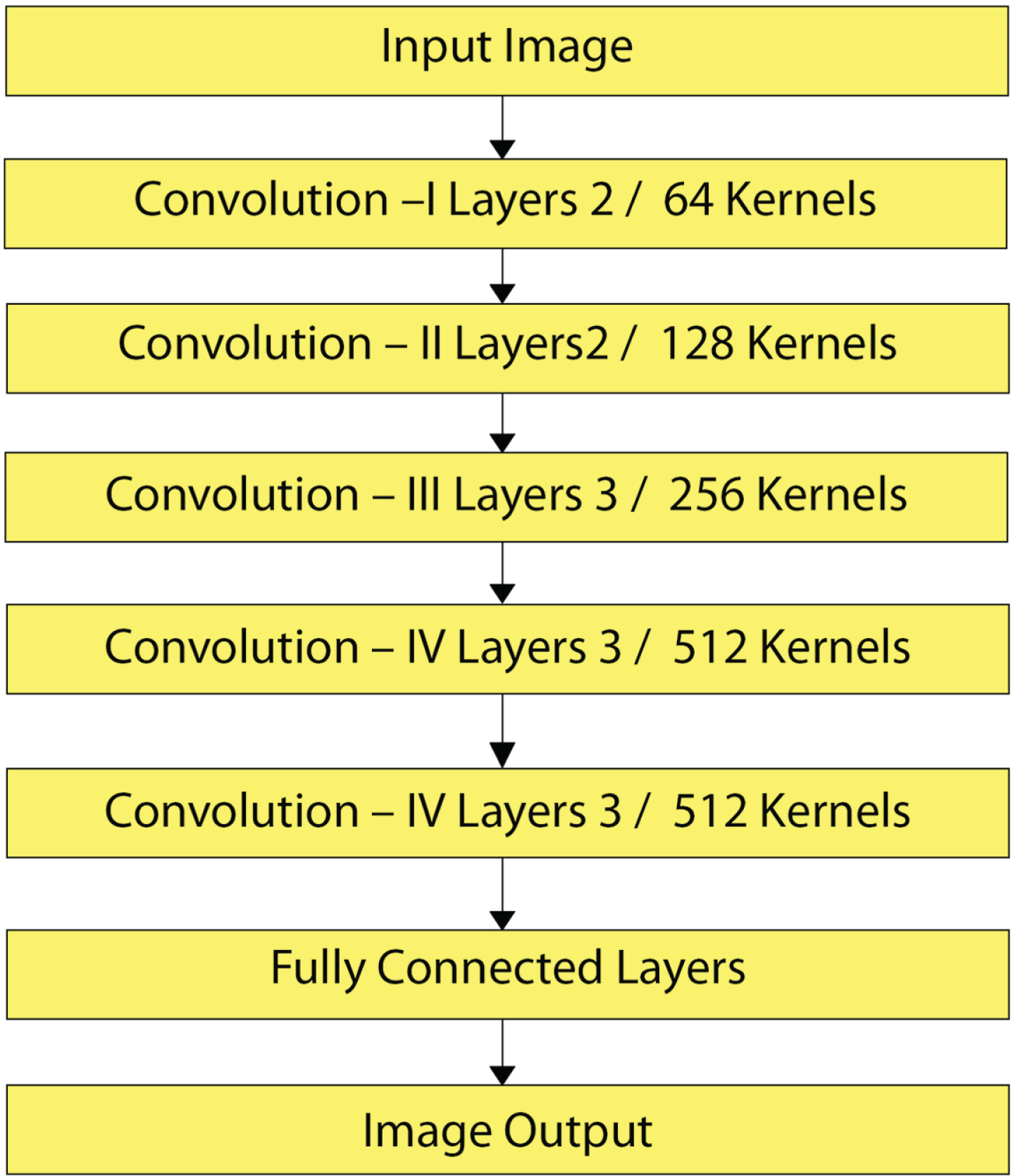
In general, a CAD machine embraces numerous stages as follows: Image Augmentation, Image Segmentation, Feature Extraction, Feature Classification, and ended with Classifier evaluation. The innovation of method is the extraction of ROI utilizing two methods and replacement of the last fully connected HR-MP-DCNN architecture layer with SVM [12]. The CAD method proposed for this work shown in Fig. 1. The sub-sections described below each block in detail.

Fig. 1

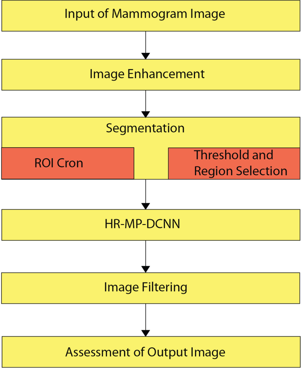
Architecture Flow chart of HR-MP-DCNN.

3.1 Image augmentation

To assist radiologists in identifying anomalies, image augmentation enhances mammographic images to increase dissimilarity and reduce noise. There is more number of strategies to improve the picture as in [13], among which is the Adaptive Contrast Enhancement (ACE). Thus ACE can able to enhance limited contrast and bring much information over the picture. It produces an excellent method for contrast augmentation of both medical and natural images. But significant noise where produced. The Contrast-Limited Adaptive Histogram Equalization (CLAHE) that is a kind of ACE, where used in this article to advance the dissimilarity in images. The disadvantages of ACE are that it happens because of the integration process, and it can over-enhance the images with noises. The CLAHE consequently used as it practices clip level for restricting the local histogram to limit the sum of contrast enrichment per pixel.

The CLAHE procedure can be concise as follows:

Divide equally sized contextual areas from the original image,

The histogram to each region has Applied an equalization,

Shrink histogram by flat of the film,

Reorganize the number clipped to the histogram,

Obtain the improved rate of the pixel by integration with histogram.

An enriched image is shown in Fig. 2 using CLAHE and its exemplification of a histogram.

Fig. 2

(a). Mass case of actual malignant (b). CLAHE Enhanced Image Extracted from HR-MP-DCNN.

3.2 Image segmentation

Image Segmentation is mainly for separating the actual images as sections that have related characteristics and their properties. The principal purpose of segmentation is to streamline pictures by giving through an effortlessly analyzable manner. The best standard methodologies for image segmentation are edge, Partial Differential Equation (PDE), fuzzy theory, threshold, artificial neural network (ANN), and segmentation depends on regions [14].

3.2.1 Thresholding process

Thresholding approaches are the modest methods for the segmenting of images—the pixels of the images separated according to the intensity level. The Global Threshold is the most common type of thresholding system. It achieved by setting a reasonable limit value (T_h). This value of (T_h) set to be the same for the entire image. The performance x (a, b) should be found from the original y (a, b) image, as shown in Equation (1) based on (Th). 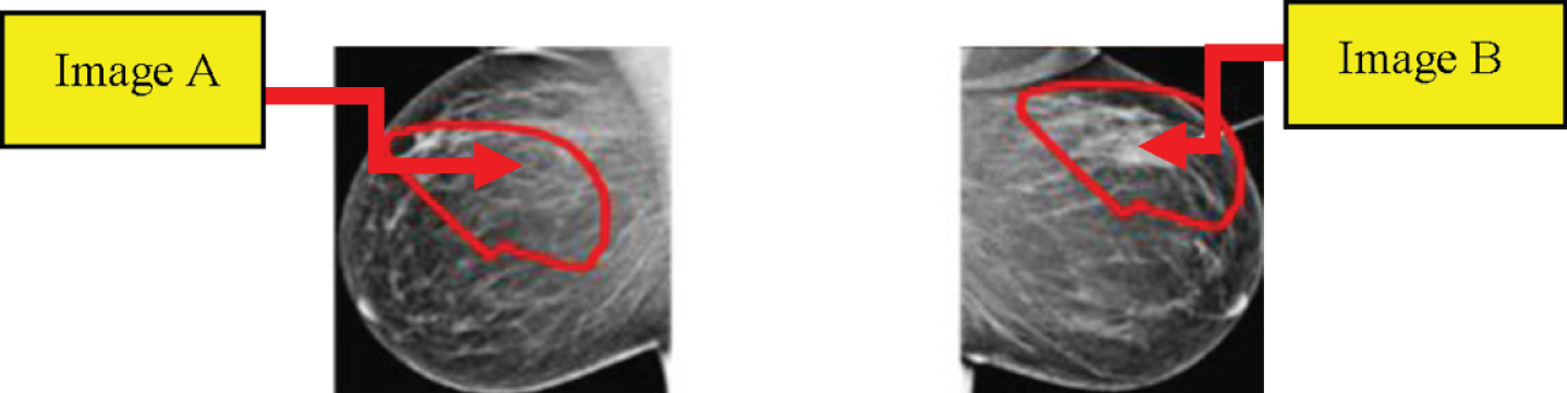$P (x, y) = [\begin{matrix} 0, if q (x, y) < T \\ 1, if q (x, y) > T \end{matrix}]$ (1)

3.2.2 Region-based segmentation method

Segmentation based on the section is modest than the other methods. It splits the image, depends on predefined criteria, into different regions. The region-based segmentation has two main types; Section Increasing, and section Splitting and Merging. The area-widening system can remove a section from the image depends upon specific predefined parameters such as severity. Area Increasing is a method of image segmentation that explores adjacent pixels and enters an area class, and no edges identified. It is also known as a form of image segmentation based on pixels, as this requires choosing the initial seed point, whereas section splitting and merging methods are contrary to the area-developing method as this operates on a whole picture. In this manuscript, two different methods extract the ROI as of the original mammogram image. In a deep neural convolutional network, the first method is to use circular contours to determine ROI. The tumours in Digital Database are formulated through Screening Mammography (DDSM) dataset and labelled using red contour, and thus the contours are physically calculated through analyzing the tumour’s pixel values and by using them to remove the area. Image from ROI manually cropped from a dataset. In the second method, the ROI calculated using the threshold and the section-based methods. In the DDSM dataset samples, the tumour labelled with red contour. The initial step to mine ROI is to determine a threshold value for the tumour section, whereas the value resolute concerning the red colour pixel. Later in some experiments, the threshold for all the images was set at 76, regardless of the tumour size. Therefore, the largest region, along with the image calculated within this range, and the tumour automatically cropped—the ROI derived by threshold and the region-based process in Fig. 3.

Fig. 3

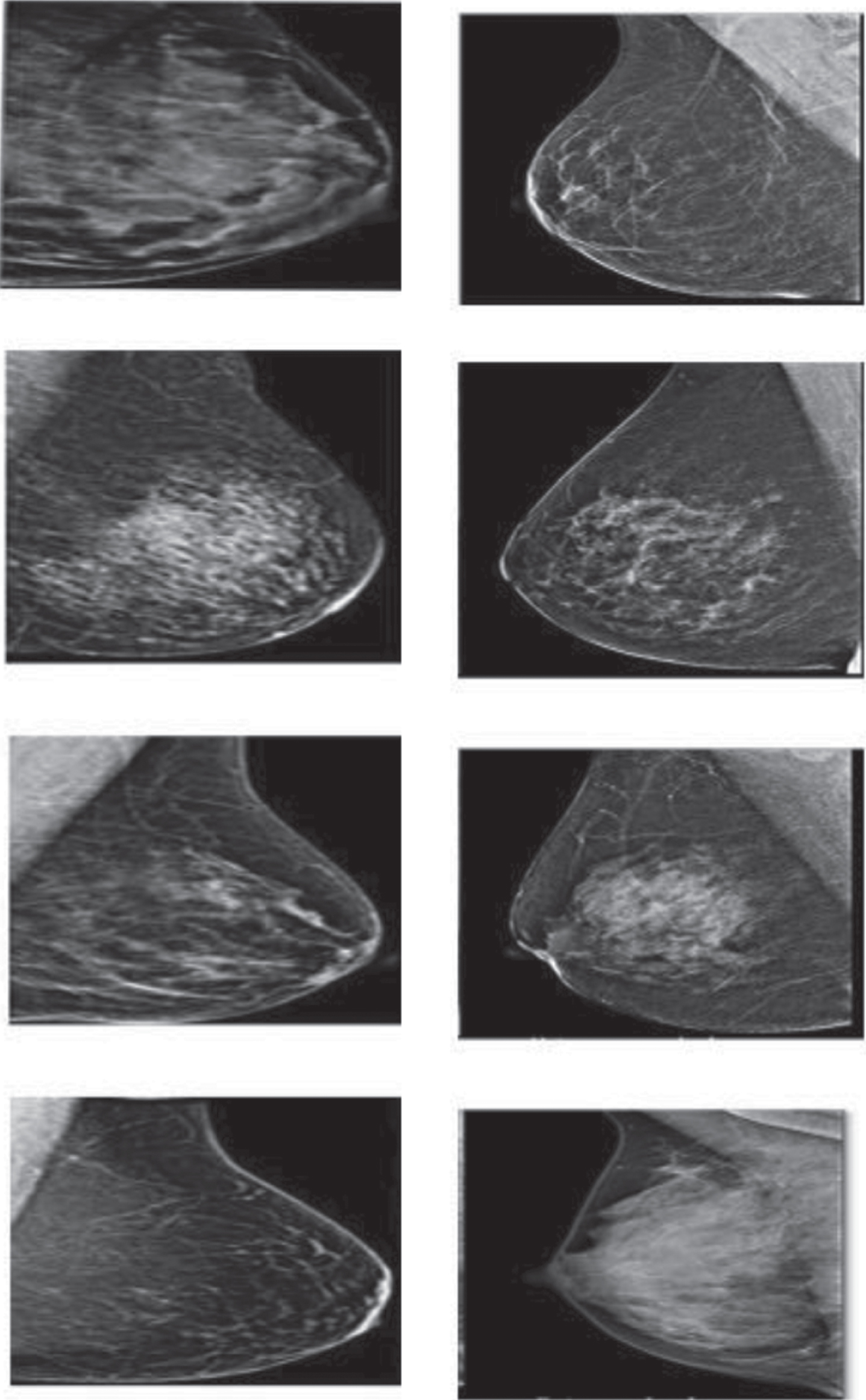
Image segmentation.

The steps of the existing method can be concise as follows:

Using the threshold technique, the original mammogram grey-scale image converted to a binary image.

Binary image objects are marked, and pixel numbers counted. Both binary objects excluded except for more significant, where the threshold-related tumour. The primary area in the area around the tumour covered in the red contour tab.

The threshold value for most significant area pixels set to “1” later the system tests all pixels in the binary image, or else all remaining pixels set to “0”.

The resultant binary image combined by actual mammographic image for receiving the last image without enchanting the rest of the breast area or some other objects into consideration

3.3 Feature extraction

There are various techniques available for feature extraction of the function phase. Due to their outstanding performance, High-Resolution Multi-View Deep Convolutional Neural Network has attracted significant attention in recent years. Accordingly, here we used HRMP-DCNN for extracting features of an image.

3.3.1 Deep convolutional neural network

A deep convolutional neural network is a classifier that takes x as an input image, often with multiple channels corresponding to different colors (e.g., RGB), and outputs the conditional probability distribution over categories P (z|y).

It achieved through a series of nonlinear functions that slowly transform the image level of the input pixel. A significant feature of the profoundly convolutional network that separates it from a multi-layer perceptron is that it relies heavily on convolutional and pooling layers that make the network invariant to the local visual input translation.

3.3.2 High-resolution multiple perspectives deep convolution neural network (HR-MP-DCNN)

Object recognition activities involving natural images usually involve only one image at a time, whereas a medical imaging test often requires a set of views. For example, obtaining views of Mediolateral Oblique (MO) and Cranial Caudal (CC) for each patient’s breast is standard in screening mammography, resulting in a set of four images. They’re referred to as R-CC, L-CC, R-MLO, and L-MLO, (Fig. 3). There is a rich literature on creating deep neural networks for data from multiple views. Most fell into a family of two. Secondly, work on unsupervised extraction of features over the multiple views is performed with the type of deep autoencoders [16]. Typically they trained a multi-view deep neural network using unlabelled samples, and utilize a network’s performance for feature extractor, tracked through standard classification.

Then again, [15] suggested specifically for classification the construction of a multi-view deep convolutional network. They proposed a motivated variant of HRMP-DCNN. The performance of This MP-DCNN measure in two steps. More number of convolutional and pooling layers was added discretely to overviews during the first step. Thus this denotes view-specific demonstration by HRi, where ‘I’ represent to view’s index. These outlook specific representations are added to form a vector [HRLEFT–CC, HRRIGHT–CC, HRLEFT–MO, HRRIGHT–MO], which is a second stage input—a fully connected layer monitored by a P(z|y) output distribution softmax layer. The entire network jointly trained with backpropagation through stochastic gradient descent. Also, due to relatively lesser size in the training data set, this uses a variety of regularization strategies to prevent overfitting behaviour, such as data increase by random cropping and dropout. Those will be described in detail later.

BIDMC-MGH and Wisconsin Screening Breast Cancer databases [19] used for the suggested models. The output measurements of the models used measured based on five parameters. AdaBoost and logistic regression were among the best scoring ones. Comparisons with other studies show the efficacy of the new system for superior breast cancer detection against the classification methods that have been tested. The following Fig. 4 represented (a) there is a circular mass in the left breast, with irregular margins. The patient recalled because to describe this mass.

Fig. 4

The four standard views used in our experiments for exams categorized (a) (b) (c).

Further, additional mammographic views and breast ultrasound were required. This mass proved to be an invasive canal carcinoma; (b) it is a natural mammogram in a woman with a breast pattern of dispersed fibro glandular tissue. No anomalies have been found; (c) this patient has a breast pattern of a distributed fibro glandular tissue. Calcified masses associated with post-surgical changes found in the posterior depth of the two breasts, near the chest wall.

3.3.3 High-resolution convolutional neural network

In object recognition and detection, it is reasonable to downscale an original high-resolution image slowly in natural images. For example, ImageNet Challenge 2018 input to the best performer’s network (classification task) was an image downscaled to 448X448 [15]. It is often done to improve computational proficiency, both in terms of processing and memory, and also this occurs because, with higher resolution images, no significant improvement has been observed.

Nevertheless, in the case of medical images, and especially for early-stage screening based on breast mammography, a downscaling of an input image is not desirable. A diagnostic clue is often a subtle finding which can be identified only at the original resolution. We propose to use aggressive convolution and pooling layers to tackle the computational issues of handling full resolution images. Firstly, in the first two convolutional layers, we use convolution layers with steps higher than one. The first layer of pooling also has an additional enormous stride than the other levels of pooling. As a result, we made lesser the size of feature maps early through the network considerably. Though this dynamic convolution and pooling lose some spatial information, the network’s parameters are modified to mitigate this loss of information during training. That is unlike input downscaling, which unconditionally loses information. Second, before concatenating, the characteristic feature maps at last row, instead of merely pulling down the feature maps and then concentrating them. It enormously reduces view-specific vector dimensionality without significant, if any, performance degradation. Using both of these approaches, we can build an HRMP-DCNN that takes as input four images of 2800x2400 pixels without downscaling.

3.3.3.1. Algorithm 1 HRMP-DCNN Detection

Input:

Fully Supervised Dataset DFS=(I, H) i NF i = 1

Weakly Supervised Dataset DWS=(I, X) i NW i = 1 3D Faster R-CNN and logistic regression parameters θ.

Initialization:

By maximizing the Equation using fully supervised detection, the objective function has maximized the log-likelihood function through nodule ground truth H for the given image I, as observed Equation (2). $\begin{matrix} L (θ) = {Log}_{P} (H \cup H^{'} | I; θ) \\ = \frac{1}{M} \sum_{m = 1}^{M} {Log}_{P} (H_{m} | I; θ) - 1 / N \sum_{n = 1}^{N} {Log}_{P} (H_{n}^{'} | I; θ) \end{matrix}$ (2)

For epoch = 1 to #Total Epochs Weakly Supervised

Training

Step 1: To obtain proposal probability, P(H_m|I; θ′) use Faster R-CNN model θ′ 0 for weakly supervised data tested from DW.

Step 2: Proposals removed with small probabilities and NMS.

Step 3: For m = 1 to M

Step 4: Each weak label

Step 5: Calculate P (z_m, Loc_m|H_m; θ) for each proposal by Equation (3).

$\begin{matrix} P (Z_{m}, {Loc}_{m} | H_{m}; θ = \frac{2}{\sqrt{2 π σ^{2}}} \\ Exp (- | Z_{m} - \frac{Z_{H_{m}} |^{2}}{2 σ^{2}}) Exp (f (H_{m}) θ_{{Loc}_{m}}) \end{matrix}$ (3)

Step 6: By Equation (4) with normalization calculate the posterior distribution $\begin{matrix} P (H_{m} | I, Z_{m}, {Loc}_{m}; θ^{'}) α P (H_{m} | I, Z_{m}, {Loc}_{m}; θ^{'}) \\ P (Z_{m}, {Loc}_{m} | H_{m}; θ^{'}) \end{matrix}$ (4)

Step 7: Employ MAP by Equation (5) $H_{m}' = {ArgMaxH}_{m} P (H_{m} | I; θ') P (Z_{m}, {Loc}_{m} | H_{m}; θ')$ (5)

Step 8: Obtain Equation (6) the expect log-likelihood function using the estimated proposal (MAP) $\begin{matrix} Q (θ; θ^{'}) = \frac{1}{M} \sum_{m = 1}^{M} 1 E_{p} (H_{m | I, Z_{m}, {Loc}_{m}; θ^{'}}) \\ [{Log}_{P} (H_{m} | I; θ) + {Log}_{P} (Z_{m}, {Loc}_{m} | H_{m}; θ)] \\ - {IE}_{Q} (H_{n | z}^{'}) [{Log}_{P} (H_{n}^{'} | I; θ)] \end{matrix}$ (6)

Step 9: Update parameter by Equation (7) $\hat{θ} = ArgMaxQ (θ; θ^{'})$ (7)

Step 10: End For

Step 11: Stop the Process

3.3.3.2. Fully supervised training

Maximizing Equation (8) the weights θ update using fully supervised data DF $\begin{matrix} l (θ) = {Log}_{P} (H \cup H^{'} | I; θ) \\ = \frac{1}{M} \sum_{m = 1}^{M} {Log}_{P} (H_{m} | I; θ) - \frac{1}{N} \sum_{n = 1}^{N} {Log}_{P} (H_{n}^{'} | I; θ) \end{matrix}$ (8)

Figure 5, a two-dimensional example of biased length sampling, where the time the tumour is present in a woman’s body depends on the rate of tumour growth and symptomatic detection potential. The crosses reflect detection times. The screen-detected case has a slow growth rate and delayed detection of symptoms

Fig. 5

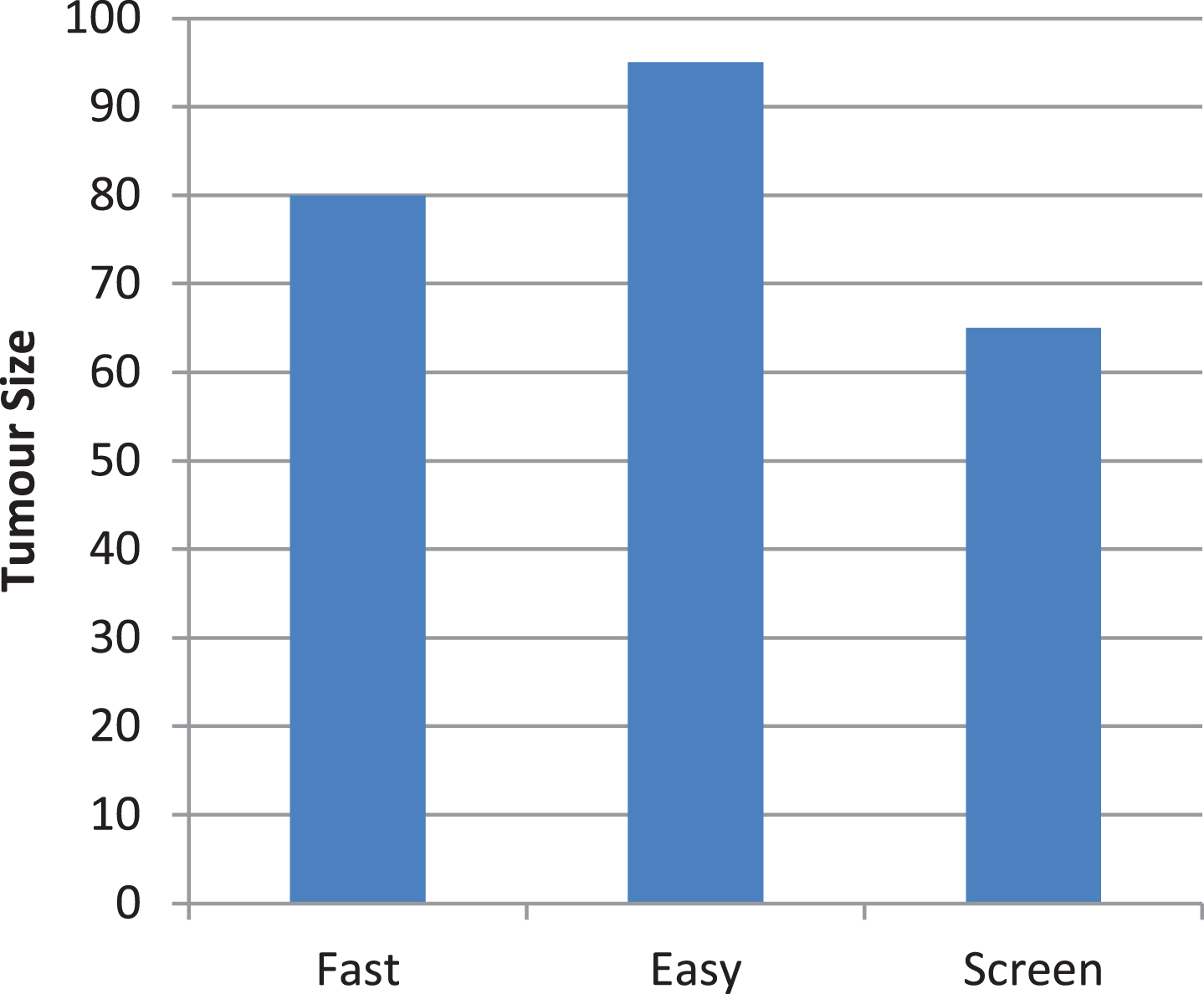
A two-dimensional example of biased length sampling.

3.3.4 Transfer learning

Firstly, HRMP-DCNN is pre-trained by using the ImageNet dataset that comprises 1.8 million original images of the process for classifying of 2,000-classes. Next, a new layer replaced by the last fully connected layer for the organization of two classes they are malignant and benign masses. Figure 6 demonstrates VGG’s fine-tuning for classifying only two groups. Some parameters must set for retraining the VGG after refinement of the fully connected layer into two classes; the number of iterations with the initial learning rate is set at 110 and 10^–3, respectively. The momentum is set at 0.9, whereas weight deterioration set at 10x10^–4. Such settings intended to ensure the criteria for the diagnosis of medical breast cancer are finely tuned—optional factors set to default values. The Stochastic Gradient Descent with Momentum (SGDM) is the optimization algorithm used.

Fig. 6

VGG Structure.

3.3.4.1. VGG

This paper examined the impact of depth of the network while keeping the filters from convolution very low. We presented that significant change should be accomplished to raise the depth to 15–20 layers. The convolution layer has a 448x448 image as input to that has a fixed size. The image is delivered through a mass of convolution layers with ReLU activations anywhere microscopic receptive field (4x4) filters have been used. The frequency of convolution is as well asset to 1. Spatial pooling achieved through five layers of max-pooling with some convolutional layers. Like AlexNet, a mass with three fully connected layers placed on top of the network’s convolution allayer. The VGG has benefits that are an efficient receptive area of the network is increased by piling several convolution layers along with small-sized kernels, thus dropping the number of factors related to use less-convolution layers by larger kernels of the same receptive region. Several configurations are of varying depth checked by the authors (8, 9, 11, and 20 levels). 1x1 filters used in one of the setups that can be view as a linear input channel revolution. It is a way of increasing non-linearity of resolution function lacking distressing convolutional layer receptive fields. One of the configurations also included a layer of LRN. According to the article, the best results for depths between 15 and 20 achieved. VGG architecture shown in Fig. 6.

3.4 Feature classification

In this stage, the ROI graded according to the characteristics as either benign or malignant. Classification The classification is supported out on the property values after performing hybrid extraction. Classification is generally well-defined as a class boundary with the purpose of mark the classes established on their stately features. For this example, the MP-DCNN classifier is in the habit of identifying the normal and abnormal cases of mammography, i.e., malignant and benign. If no prior data distribution data exists, DNN should be one of the first classification options.

3.4.1 HRMP-deep neural network

Typically, HRMP-DCNN acts as feedforward networks, with an unsupervised pre-training method by greedy layer-wise training.

Thus data flow from the input layer to the output layer without looping the feature. The key benefits of the HRMP-DCNN classifier are that the chances of losing worth are minimal during classification. In the unsupervised pre-training phase, the HRMP-DCNN technique performs only one sheet. Throughout prediction time, the HRMP-DCNN assigns a classification score f(x). Each sample input data x = [x₁,... x_n] is pass-forward. Typically f is a function that includes a sequence of computational layers expressed in Equation (9) $Z_{ij} X_{ij} W_{ij} Z_{ij} = \sum_{i} Z_{ij} + b_{j}; x_{j} = g (Z_{j})$ (9)

Where the layer input is x_i, the output layer is x_j, and the model parameters are w_ij, and the mapping or pooling function performed by g(Z_j). The propagation of layer-wise significance decomposes the classifier output f(x) for the relevance of each input part x_i, which donates to the classification result stated in Equation (10). $f (x) = \sum_{i} r_{i}$ (10)

Where r_i > 0 implies positive confirmation, which supports the classification result, and r_i < 0 is negative proof for classification, or else, it refers to as neutral indication, while the relevant element r_i is determined using Equation. The MP-DCNN General Scheme shown in Equation (11) $r_{i} = \frac{\sum_{j} z_{ij}}{\sum_{i} z_{ij}}$ (11)

The MP-DCNN is capable of investigating input coherences of the unknown feature. The HRMP-DCNN provides a learning approach to hierarchical features. Therefore high-level features have resultant from low-level features by greedy layer-wise unsupervised pertaining data. Therefore, HRMP-DCNN’s principal objective is for handling the complex functions which denote high-level abstraction.

4 Data set

4.1 Data collection

It is a retrospective report by Health Insurance Company approved by our Institutional Review Board. Consecutive screening mammograms for 139,609 patients aged 1 between 20 and 90 (mean: 57.2, std: 11.6) obtained during nine years (2010-2019) used in this research at five imaging sites affiliated to the World Medical Association.

4.2 Data statistics

We used all the data that we could gather and omitted no data unless it was collected improperly. The data split in the following way into disjoint instruction, validation, and test sets. To begin with, we sorted all patients into the data set, agreeing to the date of their advanced examination. In this order, we use the first 80% of the patients as training data, the next 10% as validation data, and the last 10% as the test data. We measure the efficiency of our model for each patient in the test set by predicting only the mark for each patient’s most recent evaluation. This way, we can accurately predict the level of accuracy that we would reach if we tested our model on future examinations. The data set includes 139,609 patients, 310,901 examinations, and 918,815 images.

Figure 7 distribution of related data with specific Bi-RAADS in preparation, testing, and test data. The following format is available for each cell in the table: number of exams/number of photos.

Fig. 7

Distribution of related data with specific Bi-RAADS.

4.3 Data-processing and augmentation

The photos were processed as follows. We state the mean as μ and standard deviation of its pixels aimed at each image. Afterward, we subtracted μ from each pixel and divided each pixel by y. Therefore, we rotated the images of R-CC and R-MO views horizontally so that the breast was always on the same side of the image. Since the images vary in size and a significant fraction of the surface of each image is empty, we cropped them all to the size of 3600/3000 pixels.

We did it on two levels. First, unify the image sizes (which we need to put into mini-batches during training) while keeping them at a similar scale and, second, avoid processing the background that does not contain any information. The crop’s location was determined as follows. First, the crop area placed on the horizontal axis to the left and the vertical axis to the centre. Noise has been added to this position to enhance the data set. Let’s denote the number of pixels between the crop area’s top border and Border_Top’s top border of the image, and define Border_Bottom and bright analogously. We drew a number from a Uniform Distribution DU (Minimum (Border_Top, 100), Minimum (Border_Bottom, 100)), and DU (0, Minimum (Bright, 100)) Top_Vertical. We have finally translated the crop area position horizontally by TopH pixels and vertically by Top_Vertical pixels. This noise was independently sampled during training each time an image used. There was no noise applied to the crop area location during validation. We fed 10 sets of 4 randomly cropped views to the network at the test time. An aggregation made the final forecast of all crop predictions. The goal of this average is twofold; first, to use information from outside the centre of the image while keeping the input size fixed; and second, to make network prediction more reliable. A small fraction of this data includes more than one image per screen. For such situations, one image per view was sampled randomly and uniformly each time during training, and testing an exam was used. The picture with the earliest timestamp always used during validation. Figure 8 description of one deep convolutional network column for a single view. It transforms the input view (a grey-scale image) into a 256-dimensional vector.

Fig. 8

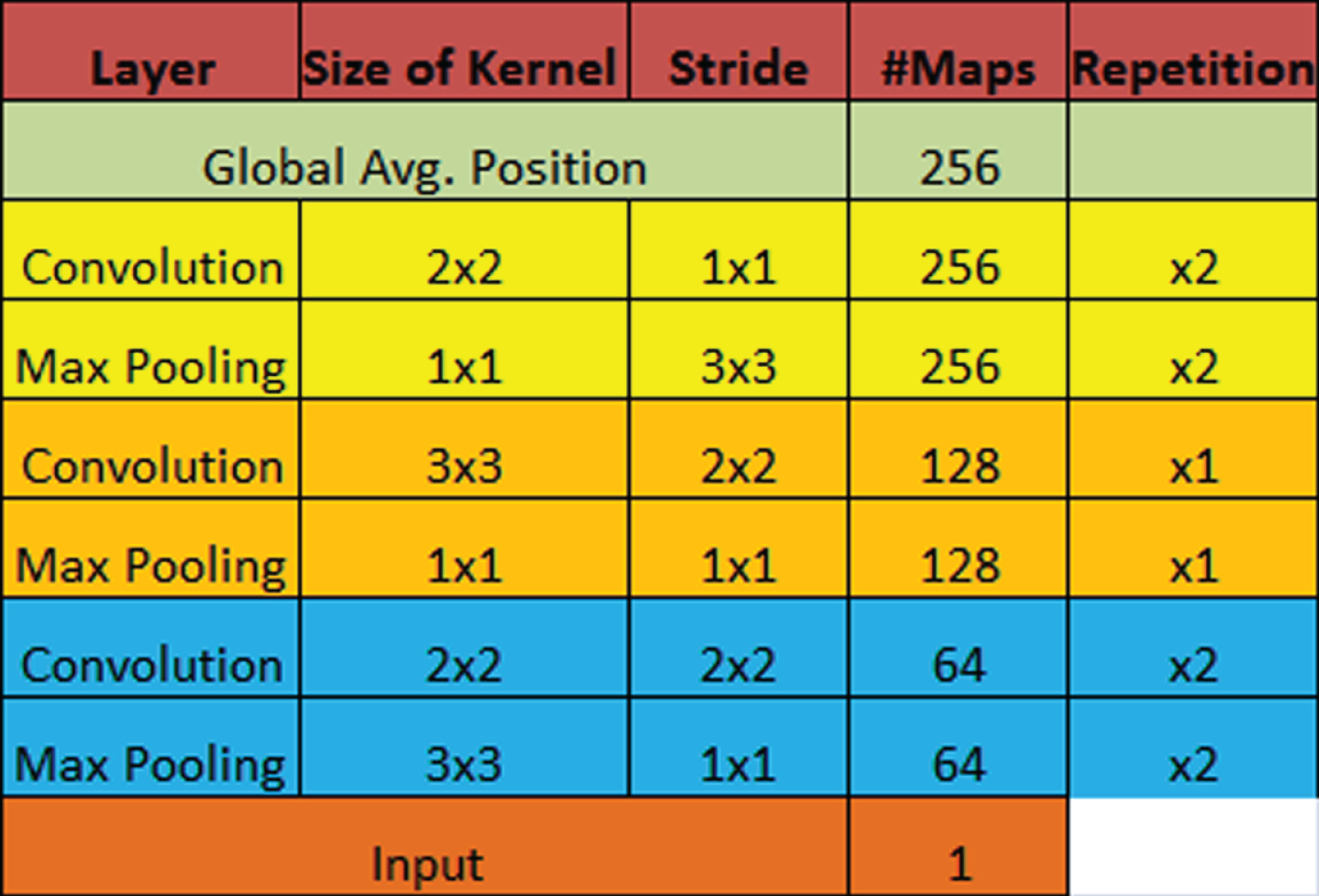
Matrix View of Convolutional Network.

Figure 9 an overview of the offered multi-view deep convolutional network, and DCN denotes the convolutional network column from Fig. 8. The arrow designates the direction of data flow.

Fig. 9

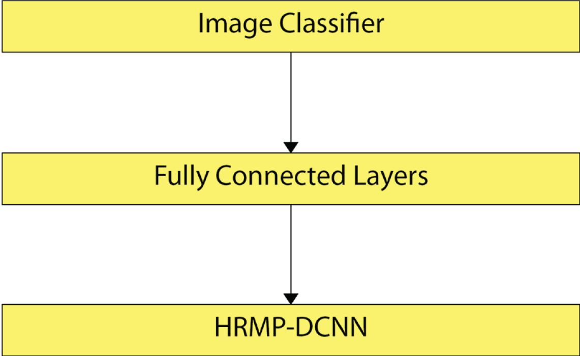
An overview of the proposed multi-view deep convolutional network.

5 Evaluation

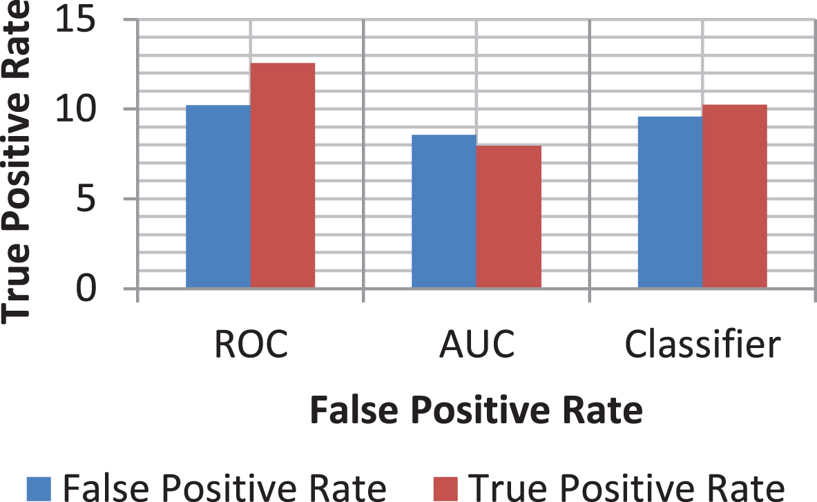
There are several evaluation tools, including the confusion matrix, the Receiver- Operating Curve (ROC), the accuracy, the area under the ROC curve (AUC), the F₁ Score, and the precision to evaluate a classifier.

5.1 The confusion matrix

The confusion matrix is a chart that visualizes the classifier’s results. An uncertainty matrix usually identified as the error matrix in the area of machine learning. Depending on the type of data, a region of images is said to be positive/negative. Besides, either True/False may be a judgment for the observed outcome. The judgment will, therefore, be one among the four categories: True Positive (TP), True Negative (TN), False Positive (FP), and False Negative (FN). The proper alternative is the uncertainty matrix diagonal. The precision accuracy is the indicator of the classifier, making the correct prediction. It gives the output Equation (12) the capacity of the entire classifier. $Accuracy = \frac{TP + TN}{TN + FP + FN + TP}$ (12)

The correctness defined as in Equation.

5.2 The receiver operating characteristic (ROC)

The ROC analysis is a simple system of estimation to identify activities. First, a medical decision-making ROC tool used; secondly, it presented medical imaging (see Table 1).

Table 1
A confusion matrix test

Class Normal Abnormal

Normal True –ve False –ve

Abnormal False+ve True+ve

Class	Normal	Abnormal
Normal	True –ve	False –ve
Abnormal	False+ve	True+ve

The ROC curve is a graph of functional points that should be viewed as a plot of True Positive Rate (TPR) as False Positive Rate (FPR) functions. The FPR and TPR, respectively, are named as specificity and responsiveness (recall). In Equations (13), (14), they described. $Sensitivity = \frac{TP}{TP + FN}$ (13) $Specificity = \frac{TN}{TN + FP}$ (14)

5.3 The area under the ROC curve (AUC)

The AUC in the medical diagnosis method, which offers a standard assessment approach, established an average of every point on the ROC curve. The AUC score should always be between ’0’ and ’1’ for the classifier result, and the model has a higher AUC rating that provides more exceptional classifier performance.

Unlike other commonly used nonlinear classifiers like random-forest or support vector machine/deep, a convolutional neural network generates a proper conditional P(z) distribution. It helps us to measure the confidence of the network in its prediction by measuring the distribution’s entropy, $H (\frac{y}{x}) = - \sum_{y^{'} \in c} p (\frac{y^{'}}{x}) {Log}_{P} (\frac{y^{'}}{x})$ (15) where y 0 iterates over all possible groups C. That the entropy, the less sure the network is about its prediction. Based on H, we can calculate the shift inaccuracy as regards network trust.

5.3.1 Precision

Precision is the ratio of appropriately estimated positive remarks to actual average anticipated comments. The low FPR corresponds to high precision. The precision determined with the resulting Equation (16), $Pr ecision = \frac{TP}{TP + FP}$ (16)

5.3.2 F1 score

F1 ranking is the accuracy and recall for the weighted average. For evaluating the classifier’s efficiency is measured statistically. Hence the score added in to account for together false negatives and false positives and F1 score set in Equation (17) $F_{1} Score = \frac{2 * Re call * Pr ecision}{Re call + Pr ecision}$ (17)

6 Result and discussions

This research proposed a new way of classification for tumours in breast cancer. It presented a new CAD program with two approaches to the systems of segmentation. The first one is manual crops, the ROI using DDSM dataset circular contours previously labelled in the dataset. The next one relies on techniques based on threshold and zone, and the threshold calculated using red contour contiguous tumour area. Thus two methods of segmentation were implemented only through the DDSM dataset.

Nevertheless, data provided already segmented for the CBIS-DDSM dataset, so there is no need for the segmentation phase was required. The features mined using MP-DCNN and pre-trained VGG design in particular. The transfer learning strategy introduced in replacing the last fully connected layer through a new layer for discrimination among two classes; malignant and benign instead of 2,000 classes. The features passed through classification MP-DCNN and SVM, wherein the last fully connected layer was associated with VM for achieving enhanced outcomes (Fig. 10).

Fig. 10

The CBIS-DDSM Dataset with computed ROC curve.

The experiments in which all the samples rotated by four angles0, 90, 180, and 270 degrees added for increasing the number of training samples to advance the precision data increase shown in Fig. 11. For DDSM samples, the accuracy of new-trained architecture for the first method of segmentation was higher when using MP-DCNN as a classifier than the second method. It has stood at 71.01%.

Fig. 11

Accuracy of ROI Cropping.

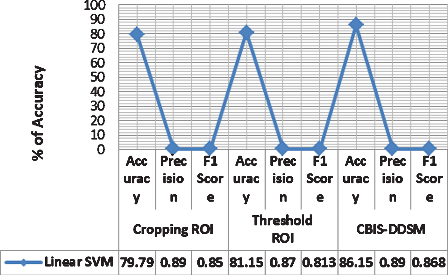
For DDSM tests, it is evident from SVM with linear kernel function attained uppermost values relative to last kernels while manually cropping the ROI. The linear SVM obtained 79% accuracy and 88% AUC accuracy. Also, the sensitivity, precision, accuracy, and F₁ score reached 76.3%, 82.2%, 85.14%, and 81.90%, respectively, that also proved to be the peak in comparison with the other kernels.

Furthermore, the SVM with a linear kernel function revealed with utmost values related to supplementary ones while using the threshold area-based technique as well. The accuracy, sensitivity, AUC, specificity, accuracy, and F₁ score reached 80.5%, 88.21%, 77.4%, 0 masses, the accuracy of the region-based technique is advanced than that of manually cropped ROI system 84.2%, 86%, and 81.5%. Therefore, while replacing previously fully connected layer of MP-DCNN with SVM to distinguish amongst malignant and benign, SVM, along with linear kernel function, achieved uppermost accuracy associated with other kernel functions for both segmentation techniques. Also, the AUC was the same for both types of segmentation. Of the ROC curves shown in Fig. 11, one can quickly notice that 8B and 8D, respectively, for first and second segmentation techniques. Besides, 69.83% and 69.57% were correctly classified while testing cropped mass samples manually, and it uses region-based segmentation systems.

In comparison, the samples had already been segmented while using the CBIS-DDSM dataset. The samples, therefore, went by the process of augmentation using CLAHE, and features extracted by using MP-DCNN. First, features characterized by using MP-DCNN, which increases the precision to 73.6% relative to DDSM samples. Although attaching a fully connected layer with SVM to increase accuracy, AUC accuracy yielded 87.2% that equals 94% . It was evident in Fig. 11. This time SVM with Medium Gaussian attained utmost values for all scores associated with other functions of the kernel, as shown in Table 1. For the CBIS-DDSM dataset, specificity, sensitivity, precision, and F₁ score exceeded 86.2%, 87.7%, 88%, and 87.1%, respectively. The entire values obtained for CBIS-DDSM were higher than those of the DDSM dataset since the CBIS-DDSM data was already segmented. The error in checking the CBIS-DDSM dataset mass samples was 23.4%. It means that 76.6% of all samples were appropriately categorized.

Eventually, the recommended CAD system was contrasted by other field articles that have similar conditions for proving the efficiency of the proposed technique, as presented in Fig. 12. The planned CAD system registered peak AUC, which was 94% for the CBIS-DDSM dataset. The last achieved AUC 81%, while later, they achieved 83% in the research studies on 219 breast lesions obtained through the medical centre at the University of Chicago. They also used as VGG, along with the process of transfer-learning. Even Jiang (2017) used BCDR-F03 dataset. Their tests performed on 736 mass cases. OTSU segmentation algorithm used to calculate the ROI. Also, the transfer learning classifies two classes as in this manuscript, instead of 2,000. When compared with the work of other researchers about the use of other MP-DCNN architectures, the highest value also reported by the AUC achieved in this suggested study.

Fig. 12

(i) DDSM (CBIS-DDSM) Curated Breast Imaging Subset (ii) DDSM-400.

6.1 Model setup

That column that corresponds to another view has an architecture defined in Fig. 9. After convolutionary layers, we implemented the rectifier feature. As well as through the data by cropping the images to random positions, we regularized the network in three ways. Next, we tied the weights in the corresponding columns, i.e., the parameters of the LN-CC and R-CC views processing columns were shared just like those of the L-MLO and R-MLO views processing columns were. Second, we added Gaussian noise to the input (near Σxi and 0.01 σ). Second, we’ve applied dropout after the fully connected layer (with a rate of 0.2). During validation and testing, we shut off the input noise and dropout. The network’s parameters were initialized and learned with the initial learning rate of 10–5. Because of our hardware’s memory limitations, the mini-batch size limited to four. Use one NVIDIA Tesla V100 GPU; we trained the network for up to 100 epochs, which takes about four weeks. After each training epoch, we measured the macAUC on the validation package. We recorded the model’s test error attaining the lowest macAUC on the validation package.

7 Conclusion

In this paper, it is examined the purpose of deep convolutional neural networks for the diagnosis of breast cancer through mammograms using mass lesions. We have made the first step towards end-to-end large-scale training of profoundly convolutional multi-view networks for breast cancer screening. This paper presented a new CAD method with two methods for segmentation. Firstly, using circular contours, the ROI is manually trimmed by the original image. It happens because the tumours marked with red contour within the DDSM dataset, whereas the region-based approach processed in next by setting through a threshold that originated to be equal to 76 then by evaluating the major area comprising this threshold. The performance of different networks evaluated on two different-size digitized mammogram databases. Whereas the first set consists of 400 DDSM images, and the other one consists of 1696. Increasing network depth, on the one hand, it points towards enhanced features in the form of filtering ability; on the further process, an increasing depth that makes the network vulnerable for numerous adverse effects like exploding gradients, and overfitting. Even though several enhancements have been proposed to the training process and network structural design to eradicate the complications enforced by increasing complexity and capacity of the models, a major necessity for active training is still a more number of data that not offered for furthermost medically focused on applications, such that the problem at hand, this gives breast cancer identification in mammals. Extensive experimental results show MP-DCNN’s effectiveness in enlightening the current state-of-art node detection systems through weakly supervised recognition data that can readily available. Although our approach based on the precise application of pulmonary nodule detection, the methodology by itself impartially general and it will be easily functional to other deep-learning medical image applications to take this as the benefit of weakly labelled data. The most recent fully connected layer in MP-DCNN has been switched by SVM to achieve greater precision. The ranking was 80.5%, 88%, 77.4%, 84.2%, 86%, and 81.5%, respectively. The proposed CAD device might be used to identify certain breast anomalies, such as MCs.

References

Kiyan

Tuba

and Yildirim

Tulay

, Breast cancer diagnosis using statistical neural networks, Journal of Electrical and Electronic Engineering 4(2) (2004), 1149–1153.

Yao

Xin

and Liu

Yong

, Neural networks for breast cancer diagnosis, IEEE, 2002.

Eddaoudi

Fatima

, Regragui

Fakhita

, Mahmoudi

Abdelhak

and Lamouri

Najib

, Masses detection using svm classifier based on textures analysis, Applied Mathematical Sciences 5(8) (2011), 367–379.

Bourdes

Valerie

, Bonnevay

Stephane

, Lisboa

Paolo

, Defrance

Remy

, Perol

David

, Chabaud

Sylvie

, Bachelot

Therese Gargi

and Negrier

Sylvie

, Comparison of artificial neural network with logistic regression as classification models for variable selection for prediction of breast cancer patient outcomes, Advances in Artificial Neural Systems, Hindawi (2010), 1–11.

Oliver

Arnau

, Freixenet

Jordi

, Marti

Robert

and Zwiggelaar

Reyer

, A comparison of breast tissue classification techniques, International Conference on Medical Image Computing and Computer-Assisted Intervention, MICCAI 2006, LNCS 4191, (2006), 872–879.

Zabalza

, Ren

, Zheng

, Zhao

, Qing

, Yang

, Du

and Marshall

, Novel segmented stacked autoencoder for effective dimensionality reduction and feature extraction in hyperspectral imaging,, Neurocomputing 185 (2016), 1–10.

Kaur

and Kaur

, Various image segmentation techniques: a review, International Journal of Computer Science and Mobile Computing 3(5) (2014), 809–814.

Ngiam

, Khosla

, Kim

, Nam

, Lee

and Ng

A.Y.

, Multimodal deep learning, International conference on machine learning (2011), 689–696.

, Maji

, Kalogerakis

and Learned-Miller

, Multi-view convolutional neural networks for 3d shape recognition, Proceedings of the IEEE International Conference on Computer Vision (2015), 945–953.

10.

Glorot

and Bengio

, Understanding the difficulty of training deep feedforward neural networks, International Conference on Artificial Intelligence and Statistics (2010), 249–256.

11.

Radisky

D.C.

and Hartmann

L.C.

, Mammary involution and breast cancer risk: transgenic models and clinical studies, Journal of Mammary Gland Biology and Neoplasia 14 (2009), 181–191.

12.

Kingma

Diederik

and Ba

Jimmy

, Adam: A method for stochastic optimization, International Conference on Learning Representation (2015), 1–15.

13.

Litton

J.K.

and Theriault

R.L.

, Chapter 65: Breast Cancer During Pregnancy and Subsequent Pregnancy in Breast Cancer Survivors. In: Harris JR, Lippman ME, Morrow M, Osborne CK, eds, Diseases of the Breast, 5th edition, Philadelphia, Pa: Lippincott Williams and Wilkins (2014).

14.

National Cancer Institute. Breast Cancer Treatment during Pregnancy (PDQ). Accessed at www.cancer.gov/types/breast/hp/pregnancy-breast-treatmentpdq#section/all on August 26, (2019).

15.

Venkataraman

and Slanetz

P.J.

, Breast imaging for cancer screening: Mammography and ultrasonography, Accessed at https://www.uptodate.com/contents/breast-imaging-for-cancer-screeningmammography-and-ultrasonography on August 26, (2019).

16.

American College of Radiology, National Mammography Database, Available at https://nrdr.acr.org/Portal/NMD/Main/page.aspx. Accessed April 13, (2017).

17.

Yankaskas

B.C.

, May

R.C.

, Matuszewski

, Bowling

J.M.

, Jarman

M.P.

and Schroeder

B.F.

, Effect of observed the change from comparison mammograms on the performance of screening mammography in a large community-based population, Radiology 261(3) (2011), 762–770.

18.

Hayward

Jessica H.

, Ray

Kimberly M.

, Wisner

Dorota J.

, Kornak

John

, Lin

Weiwen

, Sickles

Edward A.

and Joe

Bonnie N.

, Improving screening mammography outcomes through comparisonwithmultiple priormammograms, AJR Am J Roentgenol (2016), 1–7.

19.

Dhahri

Habib

, Rahmany

Ines

, Mahmood

Awais

, Al Maghayreh

Eslam

and Elkilani

Wail

, Tabu search and machine-learning classification of benign and malignant proliferative breast lesions, BioMed Research International, Hindawi Publishers (2020), 1–10.

20.

Jaber

Mustafa I.

, Song

Bing

, Taylor

Clive

, Vaske

Charles J.

, Benz

Stephen C.

, Alizadeh

Shahrooz

, Soon-Shiong

Patrick

and Szeto

Christopher W.

, A deep learning image-based intrinsic molecular subtype classifier of breast tumours reveals tumor heterogeneity that may affect survival, Breast Cancer Research 12 (2020), 1–10.