
Abstract
In terms of financial market risk research, with the rapid popularization of non-linear perspectives and the improvement of theoretical reasoning, scholars have slowly broken through the cage of linear ideas and derived new and more practical methods from non-linear perspectives to make up for the shortcomings of traditional research. Based on the support vector classification regression algorithm, this research combines the typical facts and characteristics of financial markets, from the perspective of quantile regression and SVR intelligent technology in computer science, to explore the research method of financial market risk spillover effects from a nonlinear perspective. Moreover, this research integrates statistical research, machine learning and other related research methods, and applies them to the measurement of financial risk spillover effects. The empirical analysis shows that the method proposed in this paper has certain effects, and financial risk analysis can be performed based on the risk spillover effect measurement model constructed in this paper.
Introduction
With the rapid development of the globalization of the world economy and the continuous advancement of the integration process of international finance, the economies and finances of countries around the world are closely linked with amazing breadth and depth. Since officially joining the WTO on November 11, 2001, China has made substantial progress in participating in economic globalization, which has further promoted the overall development of the economy. However, the development of economic globalization is based on an economic system dominated by developed countries. This system has a series of inequality such as development, status, and decision-making power. Moreover, financial markets are relatively special high-risk markets. A crisis in a country’s financial market can easily cause a chain reaction in the global financial market, trigger a global and systemic financial storm, and may cause economic turmoil and even paralysis in the entire country [1].
As a developing country, in order to accelerate economic development and further open up to the outside world, China has to accept the inequality rules formulated by developed countries and bear a series of financial risks brought by the economic development of developed countries. For example, the financial crisis in Mexico in 1982, the global financial crisis caused by the collapse of the Bank of Bahrain in 1995, the Southeast Asian financial crisis in 1997, the US subprime mortgage crisis that swept the world in 2008, and the European debt crisis that abused Europe in 2012. These financial crises have, without exception, caused extremely bad negative effects on China’s economic development [2].
With the continuous progress of financial liberalization, more and more countries have cancelled and relaxed financial controls. At the same time, the combination of investment activities conducted by investors around the world to diversify risks has further accelerated the integration of international financial markets. In the context of the integration of international financial markets, although there are regional and cultural differences between different countries and regions, when a country or a market is affected, markets with similar risk structures in different places will experience similar price changes.. This information spillover effect was even more pronounced during the financial crisis.
The financial crisis in the world tells us that once financial risks are not effectively controlled, it is easy to cause a chain reaction, which will cause a global and systemic financial crisis, affect the entire economic life, and even lead to chaos in the economic order and political crisis [3]. Therefore, the study of financial risk is no longer simply a discussion of cutting-edge topics in the field of economic research, but a major practical issue that concerns economic security and national security. Therefore, under the trend and background of economic globalization and China’s economic transition, correctly identifying financial risks and their transmission mechanisms, timely and accurately monitoring and measuring financial risks, taking measures to prevent and resolve financial risks, and maintaining national economic security is an important theoretical and practical significance, and an important issue that needs to be urgently resolved.
Related work
Examining the relationship between the two markets from the perspective of yield rate to study the risk spillover effects of financial markets can explain the leading and lagging relationship between the two markets to a certain extent. The literature [4] proposed stock-oriented models, which originated from the theory of exchange rate capital balance. The literature uses a return-risk analysis method, pointing out that imbalances in the domestic and foreign asset markets have an impact on the exchange rate, and the exchange rate is a key factor in maintaining and restoring the balance of supply and demand in the asset market. Therefore, there is a mutual feedback relationship between the stock market and the foreign exchange market. The literature [5] estimated the probability of financial crisis contagion through the probit model and found that countries with close economic ties are more prone to financial crisis contagion. The literature [6] used a polynomial logit model to estimate the probability of financial crisis contagion and found that there is a strong spillover effect between Latin American financial markets, but the spillover effect between Latin American and Asian financial markets is not obvious. The literature [7] studied the mean and volatility spillover mechanism of the stock and currency markets in G-7 countries. The empirical results of this literature support the view that the volatility overflow is asymmetric, that is, the fluctuation of the stock price will affect the future fluctuation of the exchange rate, but the impact of the exchange rate on the future fluctuation of the stock price is relatively weak. In the literature [8], a vector autoregressive model was used to study the stock data of Japan, the United States and Malaysia. It was found that the Malaysian stock market is showing deepening integration with the stock markets of Japan and the United States. Moreover, the impact of the Japanese stock market on the Malaysian stock market is greater than the impact of the US stock market on the Malaysian stock market. The main reason is that after the Asian financial crisis, the frequent economic and trade exchanges between Malaysia and Japan provided a material basis for the linkage between Malaysia and Japan’s stock markets. The literature [9] analyzed the daily exchange rate data of the RMB / USD exchange rate and the Shanghai Composite Index through exchange series cointegration test and VECM. It is believed that after China’s foreign exchange reform, the stock market and the foreign exchange market have a close reverse relationship, and the foreign exchange market is a one-way Granger reason for the stock market. The literature [10] studied the relationship between the exchange rate of RMB against the US dollar and the time series of various stock indexes through cointegration tests and Granger causality tests based on VAR and VECM. It is found that there is a relatively stable and long-term equilibrium relationship between the exchange rate and the stock index, and the exchange rate of RMB against the US dollar is the Granger reason for the changes in the stock index of several sectors. The literature [11] studied the stock market returns of six Latin American countries and European economies and the spillover effects of exchange rate fluctuations. The empirical results also show that the volatility of stock market returns affects the volatility of exchange rates, but the volatility of exchange rates has no effect on the volatility of stock market returns. The literature [12] used Granger causality test to study the causality relationship between the US stock market and the stock markets of 15 emerging countries. The results show that there is a one-way Granger causality test between the US stock market and the stock markets of other countries, and the spillover effects of Chinese A-shares are the most influential.
Based on the quantile, using VaR to test the risk spillover effect between the two markets can distinguish the risks faced by different economic entities. The literature [13] examined the model of income volatility spillovers that are created when impacting on emerging markets and divided the impact on emerging stock markets into local and global factors, that is, the impact of world capital markets. The literature used a vector autoregressive model [14] to study the linkage between the United States and Japan on the stock markets of emerging Asian regions and countries such as South Korea, Hong Kong, and Taiwan in the context of the Asian financial crisis. It was found that during the financial crisis, the impact of the United States and Japan on the stock markets in Asia has significantly increased. The literature [15] first proposed the concept and method of risk-Granger causality test and studied the extreme risk spillover effects of the decline of stock markets in various countries based on this method. The literature [16] discussed the risk spillover effects of the first three moments (mean, variance, and skewness) using the autoregressive conditional skewness model based on the skewed student’s t distribution. It is found that the introduction of time-varying skewness can improve the measurement effect of variance overflow. In the literature [17], the GARCH model of the GED distribution was used to estimate the VaR of rising and falling oil prices in China and the United States, and the risk spillover effects of the two oil markets were analyzed using the risk-Granger causality test. It is pointed out that whether it is rising or falling, the international oil market has a one-way risk spillover to the domestic oil market, which means that historical information on international oil market risks can be used to predict the extreme risks of the domestic oil market. Reference [18] used the multivariate condition correlation coefficient multivariate GARCH model (CCC-MGARCH) and the dynamic condition coefficient multivariate GARCH model (DCC-MGARCH) to measure the impact of the impact of the US dollar, yen, and euro on the stock market’s average and volatility by using unexpected exchange rate shocks. The empirical results of the CCC-MGARCH model show that the unexpected impact of the US dollar against the RMB exchange rate has a negative correlation with changes in Chinese stock prices, which means that the unexpected impact has a negative effect on the Chinese stock market. The literature [19] used the quantile regression method to investigate the technological spillover of FDI to Guangdong’s manufacturing industry through horizontal spillover and vertical spillover. It is pointed out that when the productivity of domestic-funded enterprises is at a high level, the technological spillover performance of FDI through the horizontal spillover pathway is playing a significant role, and it shows certain differences in the direction of horizontal spillover change and forward-related spillovers. The literature [20] used the data of 191 cities above the prefecture level in China and the quantile regression method and followed the analysis of technological gaps to analyze the impact of foreign capital on regional productivity in China. It is pointed out that as the technology gap narrows, the role of foreign investment in promoting regional productivity has gradually become smaller. When the technology gap has narrowed to a certain extent, foreign investment has mainly manifested as a competitive effect.
CoVaR theory and calculation
In order to more accurately measure the risk level of financial markets, two scholars, Adrian and Bmtmermeier [21] on the premise of in-depth study of the theory, proposed a conditional value-at-risk model (CoVaR) by considering the complex and changing interactions between markets. This model not only measures the level of risk in a single market, but also includes the contagious effects that prevail across markets [22, 23].
In the formula,
According to formula (1),
Compared with the unconditional risk VaR, the CoVaR method overcomes the deficiency that VaR cannot measure the financial risk spillover effect and greatly reduces the accuracy of risk assessment (GiulioandTolga, 2013; Liu Xiangli, Gu Shuting, 2014). Due to the different magnitudes of prices in different financial markets, the calculated CoVaR values are of course very different and cannot effectively characterize the risk spillover effect between markets. Therefore, the CoVaR needs to be standardized to obtain the risk spillover intensity
After normalization,
In order to accurately measure the risk spillover effect of the financial market, it is necessary not only to accurately measure the market’s own risk level, but also to effectively measure the maximum possible loss of the relevant market or asset portfolio when an extreme risk event occurs in a market, and then measure the market’s spillover risk. Therefore, this paper introduces a measurement method to model and analyze the intensity of market risk spillovers.
We set X to represent the risk of a certain market, and its density function is f (X). When the risk value of market j is
In the formula,
According to Equation (4),
Compared with the unconditional risk VaR, the CoVaR method overcomes the deficiency that VaR cannot measure the financial risk spillover effect and greatly reduces the accuracy of the risk assessment. It can reflect the fact that the correlation between markets during the crisis is increasing, and it is of great significance to the regulators concerned about the risks of the entire financial system. Since the unconditional risk in different financial markets varies widely, ΔCoVaR cannot fully reflect the difference in the intensity of risk spillovers in different markets. Therefore, in order to facilitate comparison, ΔCoVaR needs to be standardized to obtain the risk overflow intensity
Although CoVaR can effectively measure the risk spillover effect, it cannot characterize the sequence dependent nonlinear dependent structure. Based on this, this paper uses R-vine-copula to fully reflect the non-linear correlation structure of the sequence, and based on this, derives the CoVaR measurement method for risk spillover. However, the key to measuring financial risk spillovers based on R-vine-copula is the setting of the marginal distribution of returns. Therefore, starting from the actual operation of the financial market, this article considers the many typical facts of the return on assets to construct an ARMA-HARCH model with time-varying jump strength to better characterize the spikes, thick tails, heteroscedasticity, and jumps of the return distribution.
After the information set Ωt-1 = {R1, R2, ⋯ , Rt-1} is given, the return on assets can be expressed as:
In formula (7), μ is the mean and ɛt-1 is the residual term. In formula (8), ω is a constant term, and α and β are non-negative parameters, which reflect the dynamic process of conditional variance σ t . (α + γ) g is the sensitivity coefficient. The larger the value, the more sensitive the volatility is to market shocks, and the more persistent the volatility of the yield sequence. At the same time, γ can describe the asymmetric shock of the market.
R vine (Regular vine) was proposed by Bedford and Cooke (2001) to reflect the complex interdependent structure of many assets through general vine graphics. R vine contains a series of trees, and each side of each tree corresponds to a (conditional) double-copula (pair-copula). According to Kurowicka and Cooke (2006), a d-variable R vine consists of d - 1 trees, denoted T1, T2, ⋯ , Td-1. The node set of the m-th tree T
m
is N
m
and the edge set is E
m
. They meet the following conditions: The node set of tree T1 is N1 ={ 1, 2, ⋯ , d } and the edge set is E1; The node set of the m-th tree T
i
is N
m
= Em-1 (m = 1, 2, ⋯ , d - 1), that is, the node set of the i-th tree is the edge set of the tree; If two edges in tree T
m
are connected by edges in tree Tm+1, then these two edges must have a common node in tree T
m
.
We set d variables as X1, X2, ⋯ , X
d
, which constitutes a random vector X ={ X1, X2, ⋯ , X
d
}. Moreover, we set the marginal density of the k-th variable X
k
to f
k
(k = 1, 2, ⋯ , d), and an R-vine distribution can be defined as the joint probability density function f (x1, x2, ⋯ , x
d
) of a random vector X ={ X1, X2, ⋯ , X
d
} that can be decomposed into the following formula.
In the formula, E i is an edge set, e = j (e) , k (e) |D (e) is an edge in E i , o is a corresponding Paircopula density function, j (e) and k (e) are two condition nodes connected to edge e, and D (e) is a condition set.
However, the premise of seeking the joint density function is the R-vine structure between the known markets. Therefore, the R-vine structure needs to be found through the strongest relationship between multi-dimensional markets. In the case of small dimensions, we can traverse and search all structural figures, and select the R-vine structure with the largest likelihood value in combination with the observed data. However, once the number of variables is large, the number of possible R-vine structures will increase exponentially, and traversing search will take time and effort. Therefore, the operability of this operation is not strong (Anastasios et al., 2017). Therefore, in order to effectively construct a reasonable R-vine, it is necessary to adopt some algorithm to intelligently select the optimal R-vine structure. Based on this, this paper uses the MST-PRIM algorithm to select the optimal R-vine structure by maximizing the sum of the absolute values of the Kendall - τ coefficients of each layer of the tree (Wu Hailong et al., 2013).
After the R-vine structure diagram is determined, an optimal PairCopula function needs to be selected for each edge on the structure diagram to describe the dependencies between them. In recent years, academia has proposed a variety of model fit tests, of which the AIC and BIC test methods are commonly used in academia, and the calculation of this method is relatively simple. Therefore, this article also uses the AIC and BIC test methods to select the optimal PairCopula function from commonly used binary copula functions to describe the up-and-down dependence between assets. The calculation formula is:
In the formula, k is the number of parameters in the model, and Ioglikelihood is the likelihood value of the model.
So far, the conditional distribution density function and joint distribution density function between assets have been obtained. Finally, the risk spillover intensity between assets needs to be calculated based on R-vine. According to the copula theory, for the return series x
i
and x
j
, if the joint distribution density function and edge distribution density function are assumed to be f (x
i
, x
j
), f (x
i
) and f (x
j
), respectively, then the conditional distribution density function of sequence x
i
is:
From the properties of the Copula function, the following formula can be obtained,
Therefore, the conditional distribution function of the return series x
i
under x
j
is:
Among them, F i , F j are the edge distributions of the profit rate series, and c is the density function of the optimal PairCopula function selected by the AIC and BIC criteria:
According to the CoVaR definition,
In the formula,
After finding
Vapnik proposed a support vector machine (SVM) on the premise of in-depth study of statistical learning theory, which has inherent advantages in solving problems such as small samples, nonlinearity, and high dimensions. Earlier, SVM was widely used in discriminant analysis, and it shined in the field of pattern recognition, and achieved fruitful results. In recent years, SVM has been favored by many scholars, and its theory and methods have been further explored. Moreover, it has been widely used in classification and regression problems in various research fields, which has promoted unprecedented development in the era of machine learning. SVM is called support vector regression when solving regression problems. The basic principle is to select the kernel function to transform the chaotic and changeable mass of low-dimensional space instead of simple linear research problems into easy-to-operate linear research problems in high-dimensional space. However, it does not affect the nature of the data but only changes the relationship. In this way, fast and effective processing of linear problems in high-dimensional space is a key to revealing the nonlinear research in low-dimensional space, and the regression in high-dimensional space can pass the SVR model.
In the above formula, ω is a parameter vector, b is a threshold, and ϕ (x) is a non-linear mapping. It is obviously extremely difficult to directly estimate the parameters of the nonlinear relationship in the formula, so the model parameters can be estimated by the following optimization principle:
In the formula, λ is the penalty parameter and T is the sample size.
However, the above regression only explains the relationship of the sequences themselves. However, this article measures the risk spillover effect between markets, which is essentially the quantile of the return sequence, so SVR alone cannot achieve the expected effect. It is gratifying that the quantile regression proposed by Koenker et al. can not only accurately and effectively characterize the influence of explanatory variables on the day and shape of the explanatory variable distribution, but also solve the problem of heterogeneity in the influence of explanatory variables on different quantiles of the explanatory variables. In order to study the risk measurement between markets under non-linear relationships, Takeuchi et al. adopted a semi-parametric method to reasonably combine the two, and first proposed a support vector quantile regression (SVQR) model, and proved that this method has an inestimable advantage in the modeling of nonlinear relationships and heterogeneous effectsShim et al. used a semi-parametric method to further simplify the SVQR model, making its solution process easy to understand and easy to operate.
In the formula, τ (0 < τ < 1) is the quantile and ρ
τ
(·) is the asymmetric test function, which satisfies
The optimization problem can be solved by introducing relaxation variables and constructing Lagrange functions (Xu Qiqi, 2014).
In the formula,
According to the KKT complementary conditions, the support vector subscript sets of the SVQR model at different quantiles can be obtained.
K
t
is the t-th row of the input space kernel matrix, and the elements in the kernel matrix are
In the formula,
In the formula, df is the degree of freedom of the model.
The sample interval is from May 9, 2001 to June 24, 2019, and the indexes are the Shanghai Stock Index (SH), the Hong Kong Hang Seng Index (HSI), the US Dow Jones Industrial Index (DJIA), and the German DAX30 Index (DAX30). The daily closing prices of various stocks are used as the original sample, and all data are from a public database on the homepage of NetEase Finance. Taking into account factors such as inconsistent holidays or emergencies, data that do not coincide on the trading day are excluded, and each index receives T = 1729 sets of valid data.
In order to make the model have better econometric meaning, the natural logarithm of the sample data is taken to eliminate the heteroscedastic phenomenon of the time series. Table 1 gives the basic statistical descriptions of logarithmic daily return series of four indexes: the skewness is negative, indicating that the distribution of yield is asymmetric and left-biased; the kurtosis is much greater than 3, indicating that the tail of the yield is thicker than the normal distribution and exhibits the characteristics of a thick and thick tail. The test results of the J-B statistic have a probability value of 0, that is, at a significant level of 1%, each stock index return series is significantly different from the normal distribution. Based on this, it can be preliminarily judged that each stock index return series does not obey the normal distribution. If the normal distribution is used, it cannot accurately simulate the real situation of the stock market. The ADF test results show that the modified logarithmic daily returns of the two indices significantly reject the null hypothesis of unit roots, indicating that both series are stationary time series and can be further analyzed and econometrically modeled. The corresponding statistical diagram is shown in Fig. 1.
Basic statistical descriptions of logarithmic daily return series of four indexes
Basic statistical descriptions of logarithmic daily return series of four indexes
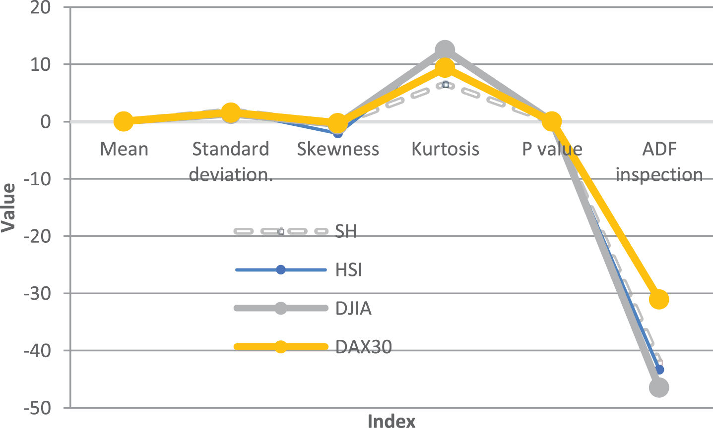
Basic statistical diagram of logarithmic daily return series of four indexes.
We use the Q-Q chart of the stock index return series to further determine the non-normality of the return series of nine stock indexes. Figures 2 and 5 show the Q-Q charts of the return series of four stock indexes.
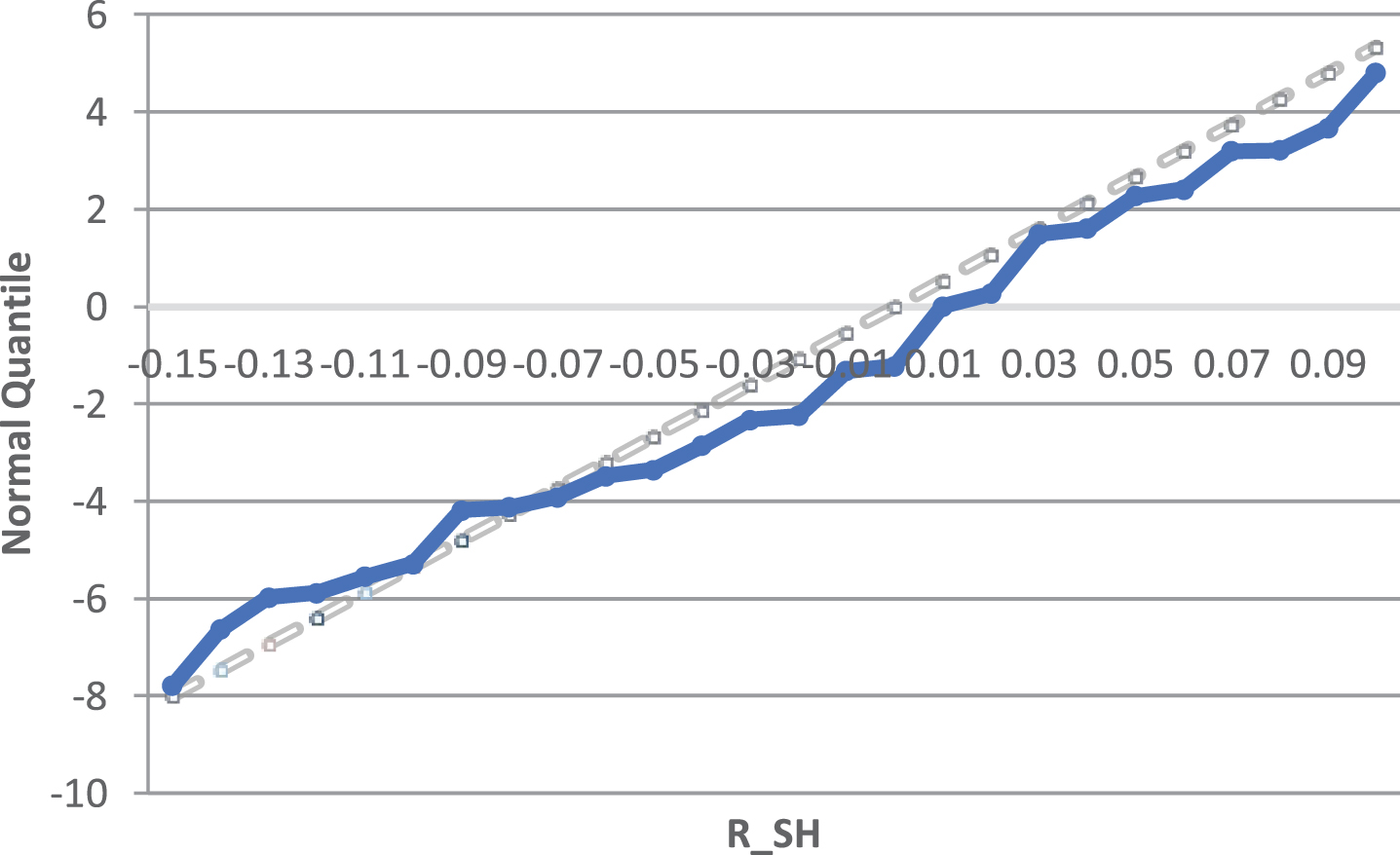
R_SH return series.
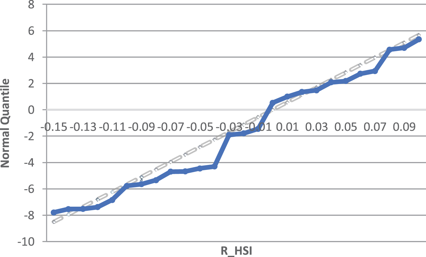
R_HSI return series.
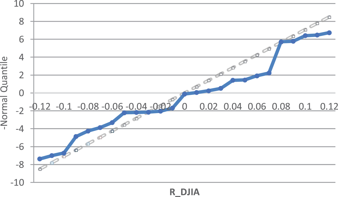
R_DJIA return series.
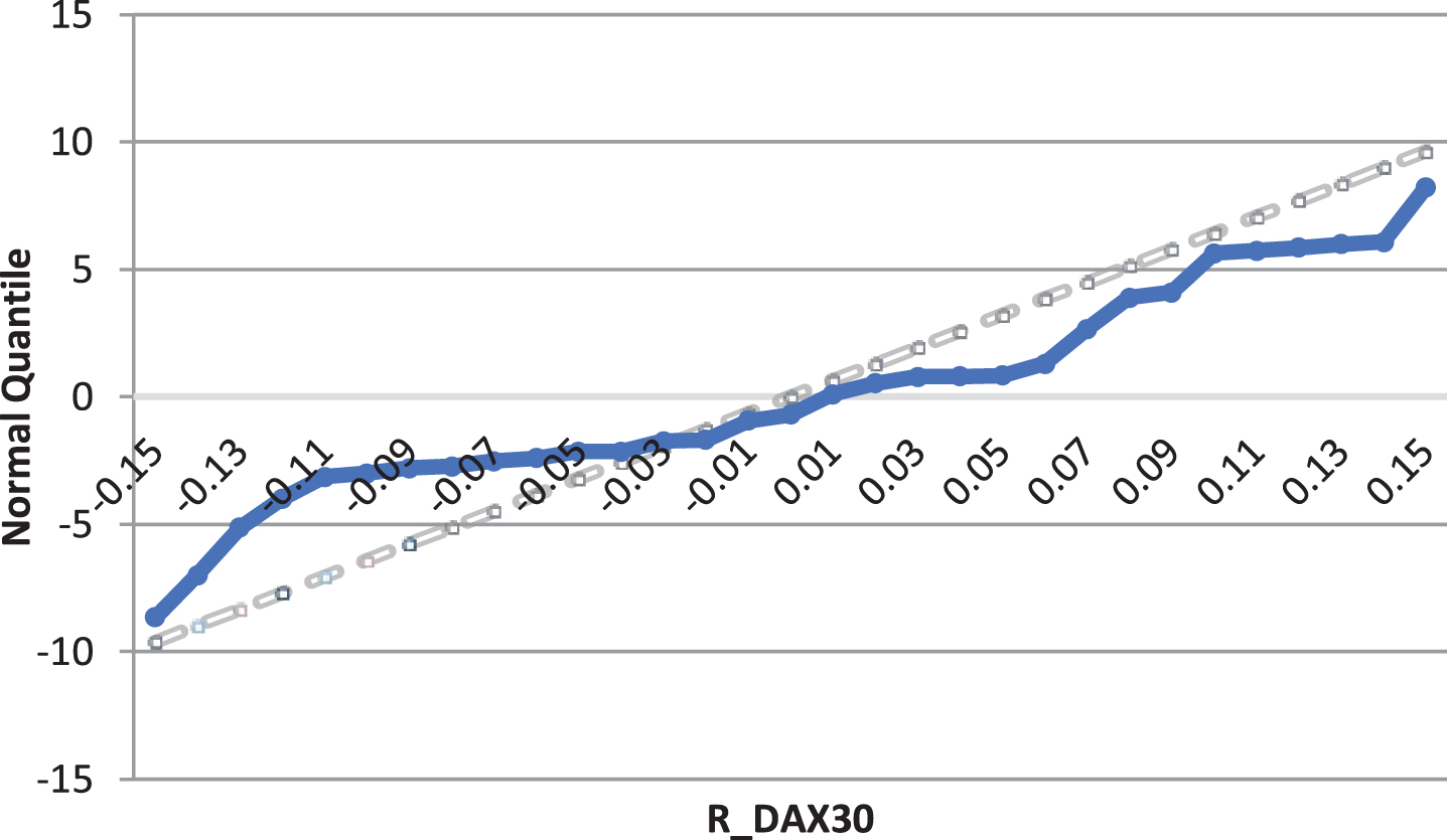
R_DAX30 return series.
It can be intuitively seen from the figure that the upper and lower tails of the logarithmic daily return series of the four stock indexes deviate significantly from the normal distribution and have significant thick-tail characteristics. That is, the logarithmic daily rate of return of each stock index has a significant -spike and thick tail feature.
Since the generalized Pareto distribution (GPD) in extreme value theory can well fit the tail data of the yield series, we use the GPD distribution to fit the upper and lower tails of the stock index yield series to the stock index yield series. Moreover, the data in the middle of the upper and lower tails are fitted using an empirical distribution. Based on the Du Mouchel 10% principle, the upper and lower tail thresholds of the logarithmic daily rate series of each stock index were determined. Then, the quantile regression method is used to estimate the scale parameter β (u) and shape parameter ξ corresponding to the GPD distribution, and the marginal distribution function of the logarithmic daily rate of return of each stock index can be obtained. After establishing the marginal distribution of each stock index’s return series, we use the Copula dependency structure function to capture the correlation structure between each stock index’s return series. According to the Copula quantile regression optimization principle, we choose the Frank-Copula function in Archimedes’ Copula function. Table 2 shows the correlation structure fitting results between the return series of each stock index. The corresponding statistical diagram is shown in Fig. 6.
Fitting results of the dependency structure between the return series of each stock index under the Frank-Copula function
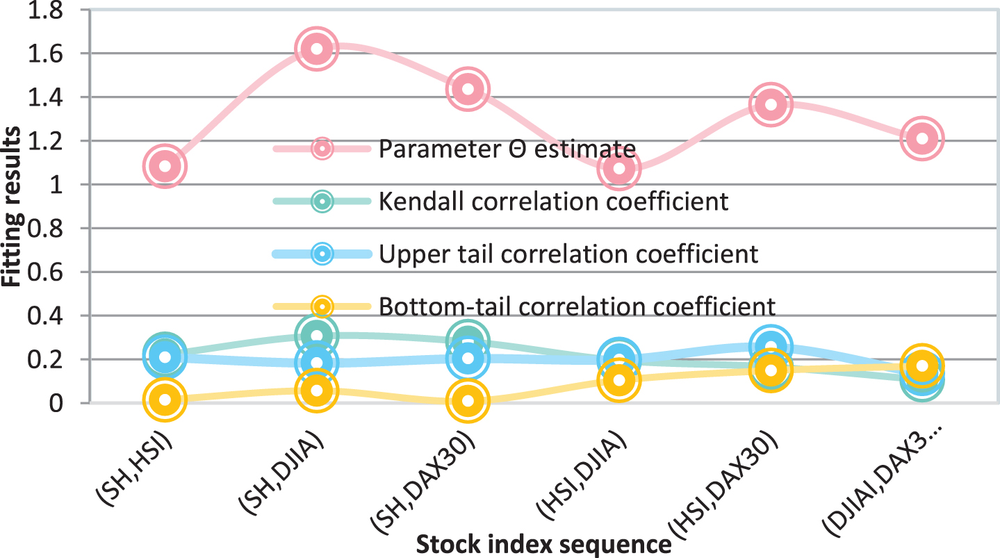
Statistical diagram of fitting results.
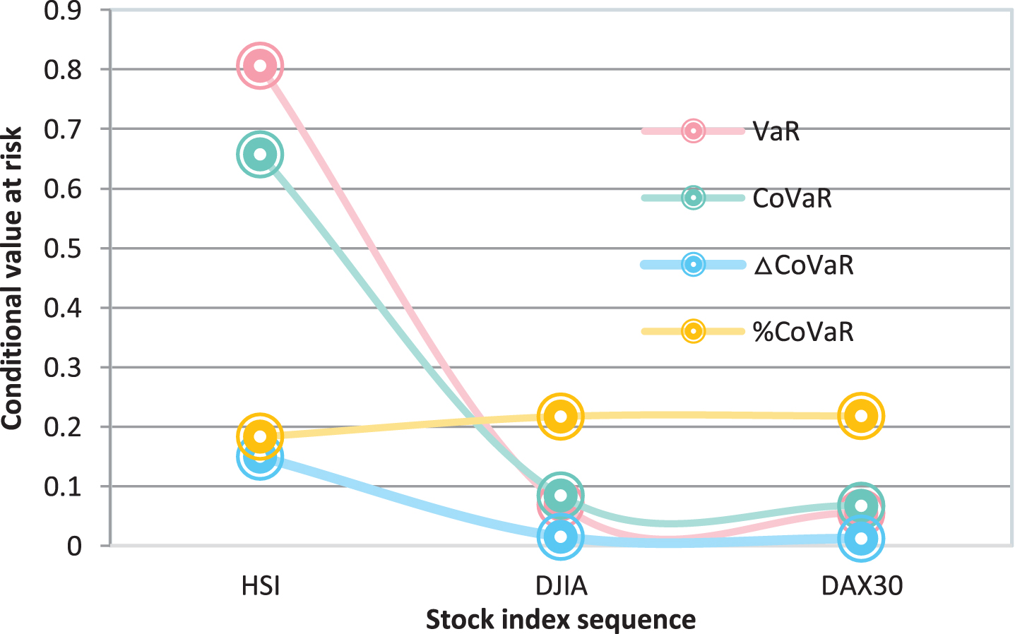
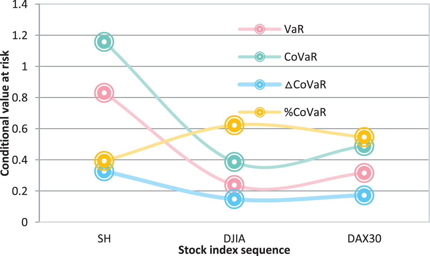
In order to examine the strength of the risk spillover effect between various stock markets, we use the quantile regression method described earlier to calculate the values of VaR, CoVaR, ΔΔCoVaR, and % CoVaR for each stock index’s return series under risk conditions. Figures 7–10 show the value of conditional risk at various conditions.
Conditional value at risk of each stock index when SH is at risk CoVaR(q = 5%).
Conditional value at risk of each stock index when HSI is at risk CoVaR(q = 5%).
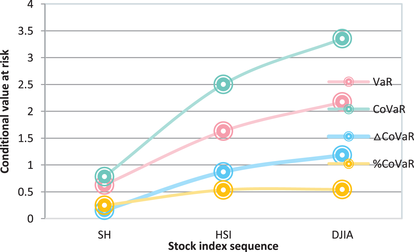
Conditional value at risk of each stock index when DJIA is at risk CoVaR(q = 5%).
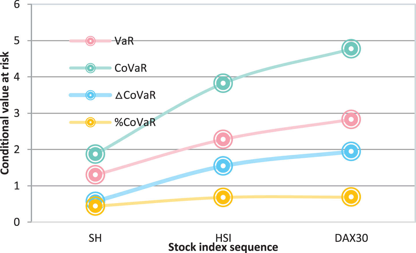
Conditional value at risk of each stock index when DAX30 is at risk CoVaR(q = 5%).
When SH is at risk, the VaR and CoVaR values of DJIA and DAX30 are very small, while the VaR and CoVaR values of HSI are relatively large. That is, the risk spillover effect of the mainland China stock market on European and American stock markets is very weak, and the risk spillover effect on the Hong Kong stock market is relatively large.
When HSI is at risk, the VaR and CoVaR values of DJIA and DAX30 are also relatively small, while the VaR and CoVaR values of SH are relatively large. That is, the risk spillover effect of the Hong Kong stock market on European and American stock markets is relatively weak, and the risk spillover effect on the Chinese mainland stock market is relatively large.
When DJIA is at risk, the VaR and CoVaR values of all stock markets are very large, and the VaR and CoVaR values of HSI and DAX30 are also much larger than SH. That is, the risk spillover effects of the US stock market on the Chinese mainland, Hong Kong, and European stock markets are very significant, and the impact on the Hong Kong and European stock markets is much greater than that of the Chinese mainland stock market.
When DAX30 is at risk, DJIA has the highest VaR and CoVaR values, followed by HSI, and SH is the smallest. That is, the European stock market has a relatively large impact on the US stock market, it has a middle-level impact on the Hong Kong stock market, and a weak impact on the mainland Chinese stock market.
In all cases, the conditional value-at-risk CoVaR of each stock index return sequence is greater than the corresponding unconditional value-at-risk VaR, indicating that the risk event of one stock index has a positive risk spillover effect on other stock markets. The highest risk spillover intensity% CoVaR is 68.7%, and the lowest is 18.3%. That is, the unconditional value-at-risk VaR significantly underestimates financial market risk.
In all cases, the VaR and CoVaR of SH are much smaller than the VaR and CoVaR values of other stock indexes. The reason is that the correlation coefficient between the bottom end of each stock market and the Shanghai Stock Index is relatively low, making the financial market in mainland China less responsive to European and American financial events. It further shows that China’s financial market is much less open than other financial markets.
Relevant research works based on traditional financial theory has not played its intended guiding role. Because there is still a certain gap between theory and practice, the practical effect of theoretical research in risk management is usually unsatisfactory, and even more, it causes inestimable losses. The conclusions of the research on risk spillover effects in this paper can not only provide decision-making basis for the related work of the risk management department, but also provide special substantive guidance for the reasonable portfolio of investors to avoid risks and reduce losses, thereby promoting the vigorous development of China’s financial market and providing a guarantee for the stable operation of global financial markets. Therefore, the conclusions of this paper on the research of risk spillover effects from a non-linear perspective are profound and significant for theoretical reference and practical guidance.