Simulation of English teaching quality evaluation model based on gaussian process machine learning

Abstract

The efficiency of traditional English teaching quality evaluation is relatively low, and evaluation statistics are very troublesome. Traditional evaluation method makes teaching evaluation a difficult project, and traditional evaluation method takes a long time and has low efficiency, which seriously affects the school’s efficiency. In order to improve the quality of English teaching, based on machine learning technology, this study combines Gaussian process to improve the algorithm, use mixed Gaussian to explore the distribution characteristics of samples, and improve the classic relevance vector machine model. Moreover, this study proposes an active learning algorithm that combines sparse Bayesian learning and mixed Gaussian, strategically selects and labels samples, and constructs a classifier that combines the distribution characteristics of the samples. In addition, this study designed a control experiment to analyze the performance of the model proposed in this study. It can be seen from the comparison that this research model has a good performance in the evaluation of the English teaching quality of traditional models and online models. This shows that the algorithm proposed in this paper has certain advantages, and it can be applied to the practice of English intelligent teaching system.

Keywords

Gaussian process machine learning English teaching quality evaluation model

1 Introduction

For a long time, our country has used the test scores of students to measure the quality of school teaching. In particular, high schools take the rate of college entrance examination as the only standard to measure the quality of school teaching. This evaluation system only pays attention to the differences in school achievements and does not pay attention to the basic school conditions, such as differences in student quality, education funding, and teachers. This evaluation method is not objective and unfair. On the one hand, it is easy to attack the enthusiasm of students with poor learning foundations, which is not conducive to the overall development of students. On the other hand, it is easy to induce parents to form a “school choice fever”.

In recent years, China’s economic strength has made great progress, people’s lives are getting better and better, and children’s education is receiving more and more attention from the country and the people. As the cornerstone of cultivating the motherland’s future hopes, the school carries the motherland’s strong dream of development and also bears the ardent hope of parents. In the development and construction of the school, the quality of teaching is a measure of the quality of the school, and it reflects the reputation of the school and directly affects the future of students. The good or bad of the school lies in how excellent the students it trains, and its views have been recognized by more and more people. Therefore, many scholars have begun to study and formulate measures to improve the quality of teaching. The purpose is to maintain teaching order and improve teaching quality. At present, there are still many problems in the existing teaching quality evaluation system in China. For example, there are too few evaluation bodies to reflect the demands of all aspects [1]. Moreover, the evaluation index cannot reflect the characteristics of each appraiser, and the evaluation index cannot be changed according to the situation; Therefore, the evaluation method still uses the traditional paper-based operation, which has the disadvantages of low efficiency. Therefore, it is very urgent to realize a set of high-efficiency teaching quality evaluation system that can reflect the demands of all parties of evaluation and reflect the characteristics of all parties to evaluation [2]. At present, the school mainly uses the method of combining student evaluation and school leader listening evaluation as the basis of teaching quality evaluation. Due to the many affairs of school leaders and their multiple roles, the use of the evaluation of lectures will inevitably affect the leadership energy. The efficiency of students’ evaluation method using paper evaluation forms is relatively low, and evaluation statistics are very troublesome [3]. This kind of evaluation method makes teaching evaluation a difficult project. This evaluation method takes a long time and has low efficiency, which seriously affects the school’s efficiency. Eventually, it caused the teaching evaluation to become formalism and could not improve the teaching effect. Therefore, the school hopes to use existing resources to design and produce a set of excellent teaching evaluation systems, so as to strengthen the management of teaching quality and better improve the quality of school education. At present, the campus network of Xinke Senior Middle School has covered the whole school, and the use of the network for office work has been popularized, so the use of the network for teacher evaluation has also become a development trend [4]. The current evaluation method for filling in the paper evaluation form is inefficient. On the contrary, the use of computer systems to achieve teaching evaluation can greatly reduce the statistical engineering volume of teaching evaluation, make evaluation more convenient and quicker, and is suitable for statistical analysis of large samples. Combining the current excellent computer system platform and using machine learning theory to design and implement an evaluation system based on machine learning evaluation algorithm is of great practical significance to the current teaching quality evaluation.

2 Related work

In the study of teaching quality evaluation, countries such as Britain, the United States and Japan started earlier than China and proposed relevant theories and methods, such as multiple intelligence theory, constructivism theory, and Taylor evaluation model. The literature [5] proposed and formulated a scoring standard on a five-point scale. The literature [6] provides a theoretical basis for the standardization of educational measurement, which marks the maturity of educational measurement. The evaluation model of the literature [7] mainly includes the evaluation with the state as the carrier, the self-evaluation with the school as the carrier, and the self-supervision evaluation in the form of social competition. The literature [8] proposed a “dual-track evaluation model” and built a multi-element, objective, and transparent evaluation system combining internal evaluation and external evaluation. In China, Beijing Normal University is the first to start relevant research work on the evaluation of teaching quality in universities. The evaluation of teaching quality in colleges and universities is a multi-level, multi-objective optimization problem, and the evaluation involves a lot of content, and the influencing factors and teaching quality present a complex nonlinear relationship, so it is difficult to accurately describe it with a certain mathematical model [9]. At present, the evaluation index system of college teaching quality evaluation is mainly based on teaching attitude, teaching content, teaching methods, etc. After quantization, these indicators are used as input feature vectors for related methods and models. The literature [10] proposed an improved Apriori algorithm to mine the data of the teaching system to evaluate the teaching level of colleges and universities. The literature [11] uses the support vector machine for classroom teaching quality evaluation model to study the existing classroom teaching quality evaluation data samples and evaluate the classroom teaching quality. The literature [12] used genetic algorithm to optimize the parameters of the support vector machine for college teaching quality evaluation model, which improves the accuracy of teaching quality evaluation. The literature [13] used BP neural network to establish a teaching quality evaluation model for training. It is proved that the BP neural network method has strong maneuverability, which not only avoids the complexity of the evaluation process, but also solves the problems of the subjectivity and excessive randomness of the analytic hierarchy process. Ge Chun used the principle of genetic algorithm to select the best individual to initialize the optimal weights and thresholds for the BP neural network and improved the accuracy of classroom teaching quality evaluation through data training. Through the research of the above related neural network technology and the evaluation of teaching quality in colleges and universities, although certain research results have been achieved, there are still some deficiencies. Existing evaluation methods and models have many problems, such as the difficulty of determining the index weights of the analytic hierarchy process. Moreover, the subjectivity and randomness of the fuzzy comprehensive method are too strong, the decision tree model is prone to overfitting, and the optimization speed of the grid search method of support vector machines is slow. Meanwhile, the convergence speed of the BP neural network is slow, and BP neural network tendency to fall into the local minimum, and it has the limited computing power and modeling representation capabilities. In addition, the evaluation indicators mostly use the teaching attitude, teaching content and other quantitative processing as the input feature vector of the model, which leads to the lack of comprehensiveness.

After the 1980 s, with the gradual development of computer technology, programming language, network communication and other technologies, some European and American countries have developed many network teaching evaluation systems, such as the evaluation software IAS and personal development system IDEA used by the University of Washington. These colleges and universities use the school network for some evaluation of the teaching process, and have obtained correct results, such as the Virtual-U and BIACKBOARD systems developed by the Si-mon Fraser University in Canada, and the WebCT system developed by the University of British Columbia [14]. These practically used systems are generally equipped with the function of teaching evaluation. For example, the literature [15] provided the evaluation function of course learning. Compared with the United States, the United Kingdom, Canada and other countries, our teaching evaluation research and application research have been slow to develop. In the 1960 s, the Ministry of Education issued the “Administrative Measures on Teachers in Primary and Secondary Schools”, which advocated that each teacher should be evaluated by the county-level education administrative department in terms of teachers’ ideological politics and the actual situation of teaching. After 1978, many teachers in China ’s teaching staff did not undergo professional vocational training. At that time, the teaching quality requirements only focused on teachers ’knowledge of textbooks [16]. From 1978 to the early 1980 s, China’s teaching evaluation system gradually began to be established. In 1986, the Ministry of Education promulgated the “Training Regulations for Teachers’ Duties”, which called for a comprehensive assessment of teachers. In 1995, the Ministry of Education promulgated the “Teacher Qualification Regulations.” In 2000, the State promulgated the “Implementation Measures for Teacher Qualification Regulations,” which marked the start of teacher qualification assessment work in China [17].

3 Proposal of mixed Gaussian kernel function

Gaussian distribution has very important analytical properties, but the use of Gaussian distribution to analyze the actual data set will have great limitations. The use of a simple Gaussian distribution for complex data in practice does not adequately describe its structural characteristics. However, if enough Gaussian distributions are used to adjust the mean, variance, and mixing coefficients of different Gaussian distributions, it can describe complex probability density forms. The mixed Gaussian model is a mixed model that linearly combines multiple Gaussian distributions. It usually treats the distribution of a series of random samples as a superposition of a set of Gaussian distributions. If the number of Gaussian components is assumed to be K, the mixed Gaussian model can be expressed as [18]: $p (x) = \sum_{k = 1}^{K} π_{k} N (x | μ_{k}, \sum_{k})$ (1)

Among them, the weight of each component is π_k, which is called the mixing coefficient. Each component is an independent Gaussian distribution, and its probability density function is: $\begin{matrix} N (x | μ_{k}, \sum_{k}) = \frac{1}{{{(2 π)}^{\frac{D}{2}} | \sum_{k} |}^{\frac{1}{2}}} exp \\ {- \frac{1}{2} {(x - μ_{k})}^{T} \sum_{k}^{- 1} (x - μ_{k})} \end{matrix}$ (2)

Since each Gaussian component is normalized, it is easy to obtain: $\sum_{k = 1}^{K} π_{k} = 1 and 0 \leq π_{k} \leq 1$ (3)

Moreover, the edge probability of the model can be calculated as follows: $p (x) = \sum_{k = 1}^{K} p (k) p (x | k)$ (4)

By comparing equation (4) with equation (1), p (k) = π_k can be obtained, which represents the a priori probability of the k-th Gaussian component. is the probability distribution of x with respect to the k-th component. Then, according to the Bayesian criterion, the posterior probability distribution of k with respect to x can be obtained: $p {k | x} = \frac{p (k) p (x | k)}{p (x)} = \frac{π_{k} N (x | μ_{k}, \sum_{k})}{\sum_{j = 1}^{K} π_{j} N (x | μ_{j}, \sum_{j})}$ (5)

If $π = {π_{1}, π_{2}, \dots, π_{K}} μ = {μ_{1}, μ_{2}, \dots, μ_{K}} \sum = {\sum_{1}, \sum_{2}, \dots, \sum_{K}}$

Then, the Gaussian mixture model is controlled by the parameter π, μ, ∑. The random variable is X ={ x₁, x₂, ⋯ , x_N }, and the log-likelihood function of π, μ, ∑ is: $Inp {x | π, μ, \sum} = \sum_{n = 1}^{N} In {\sum_{k = 1}^{K} π_{k} N (x_{n} | μ_{n}, \sum_{n})}$ (6)

The parameter π, μ, ∑of the model can be solved by maximizing the likelihood function. However, compared to the univariate Gaussian distribution, the Gaussian mixture distribution involves multiple Gaussian components, contains many unknown parameters, and it is difficult to obtain a closed solution. Expectation maximization (Expectation Maximization) can be used to treat many unknown parameters as hidden variables and solve the model [19].

The mixed Gaussian model is used to explore the distribution characteristics of the samples, and the data samples are regarded as the superposition of a group of Gaussian distributions. Moreover, by solving the mean, variance and mixing coefficient of each Gaussian component, the probability density distribution of the sample can be accurately described, and the distribution characteristics of the sample can be captured.

The general form of the Gaussian distribution function used to describe the sample probability density is: $\begin{matrix} N (x | μ_{k}, \sum_{k}) = \frac{1}{{(2 π)}^{\frac{D}{2}} | \sum_{k} |^{\frac{1}{2}}} exp \\ {- \frac{1}{2} (x - μ_{k})^{T} \sum_{k}^{- 1} (x - μ_{k})} = \\ \frac{1}{{(2 π)}^{\frac{D}{2}} | \sum_{k} |^{\frac{1}{2}}} exp {- \frac{1}{2} (^{Δ} \sum_{k} (x - μ_{k}))^{2}} \end{matrix}$ (7)

If M = ∑_k, then $Δ_{M} (x_{i}, x_{j}) = \sqrt{{(x_{i} - x_{j})}^{T} M^{- 1} (x_{i} - x_{j})}$

Among them, x_i and x_j are all sample vectors in D-dimensional space. This is the form of Mahalanobis distance. When the Gaussian distribution is used to explore the probability density distribution of the sample, the Mahalanobis distance is also used in the formula to obtain the sample distribution characteristics [20]. Therefore, the Mahalanobis distance can be used to effectively analyze the distribution characteristics of the sample. The specific form of Mahalanobis distance is: $\begin{matrix} Mahanalobis (x_{i}, x_{j}) = \\ \sqrt{{(x_{i} - x_{j})}^{T} \sum_{k}^{- 1} (x_{i} - x_{j})} \end{matrix}$ (8)

It can be seen that when ∑_k is the identity matrix, the Mahalanobis distance is just equal to the Euclidean distance between x_i and x_j, and its specific form is Eauclidean (x_i, x_j) =∥ x_i - x_j ∥. Therefore, Euclidean distance is a special form of Mahalanobis distance. However, the distance form defined by Euclidean distance is fixed for the distance between two points with fixed coordinates in space and does not change with the change of the sample distribution where it is located. Therefore, the Euclidean distance does not take into account the distribution characteristics of the sample, and the effective information of the sample is not fully utilized [21-23].

The sample points in Figs. 1 and 2 are randomly generated according to two different normal distributions Gaussian₁ and Gaussian₂. Figure 1 describes the Euclidean distance about x₁ with equidistant dashed lines, and Fig. 2 describes the Mahalanobis distance about x₁ in the Gaussian distribution Gaussian₁. For two points x₂ and x₃ in different distributions, d₁ > d₂ is obtained according to the Euclidean distance in Fig. 1, but d₁ < d₂ is obtained according to the Mahalanobis distance in Fig. 2. Since x₂ and x₁ are in the same sample distribution, the similarity between x₂ and x₁ should be greater, and the relationship between x₂ and x₁ should be closer than the relationship between x₃ and x₁. That is, the relationship between the sample distance d₁ should be closer, that is, the sample distance is smaller than d₂. From the above, it can be seen that the Mahalanobis distance is better than the Euclidean distance to reflect the distribution characteristics of samples and the relationship between samples. In the training and learning process of samples using machine learning methods, it is very important to correctly analyze and use the distribution characteristics of samples. Therefore, the Mahalanobis distance can be used to explore the connections between samples, and the distribution characteristics of the samples can be incorporated into the training of the model to improve the accuracy of the model.

Fig. 1

Euclidean distance.

Fig. 2

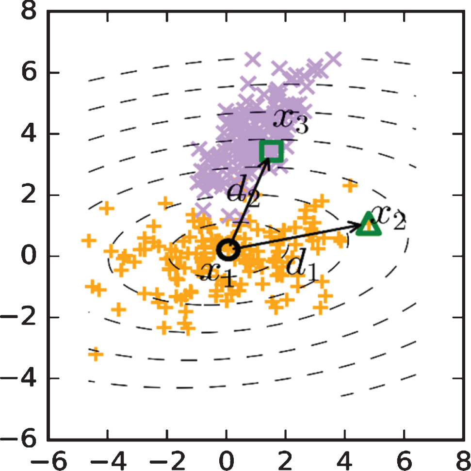
Mahalanobis distance.

In the figure above, ^′ + ′ and ^′ × ′ respectively represent samples that follow two different Gaussian distributions. However, in the sample training process, random samples often have different distribution characteristics, it is difficult to put any two samples in the same distribution to calculate the Mahalanobis distance about covariance. Moreover, using the same distribution to predict the probability density of samples is difficult to achieve good results in complex data formats. However, as mentioned earlier, for complex data structures that cannot be described correctly using simple Gaussian distributions, mixed Gaussian distributions can be used. By treating randomly distributed samples as a mixture of multiple Gaussian distributions, the correct probability density distribution of the samples is infinitely approximated. The probability density function of the mixed Gaussian distribution is: $p (x) = \sum_{k = 1}^{K} π_{k} N (x | μ_{k}, \sum_{k})$ (9)

The mixed Gaussian distribution defines the superposition of a set of Gaussian components. Among them, π_k is the mixing coefficient, that is, the proportion of each Gaussian component in the entire sample. Then, when the sample distribution is regarded as the superposition of a group of Gaussian distributions, for any two points in the sample, the Mahalanobis distance of the two points for each Gaussian component can be found. After that, through the linear superposition of the mixing coefficients, a new form of distance representation is obtained, namely, the mixed Gaussian distance: $\begin{matrix} Δ GMM (x_{i}, x_{j}) = \sum_{k = 1}^{K} (π_{k} Δ_{\sum_{k}} (x_{i} - x_{j})) = \\ \sum_{k = 1}^{K} π_{k} \sqrt{{(x_{i} - x_{j})}^{T} \sum_{k}^{- 1} (x_{i} - x_{j})} \end{matrix}$ (10)

π_k is the mixing coefficient obtained by the mixed Gaussian model, that is, the proportion of the kth Gaussian component in the sample distribution. ∑_k is the covariance matrix in the k-th Gaussian component.

Through the mixed Gaussian model, the distribution characteristics of the sample are explored, and the distribution of the sample is regarded as the superposition of a series of Gaussian distributions. Based on each weighted Gaussian component, the mixed Gaussian distance between the samples is calculated. Compared with the Euclidean distance, it fully considers the distribution characteristics of the sample and uses the effective information of the sample.

Among the many kernel methods in the field of machine learning, the most commonly used kernel function is the Gaussian kernel function, and its specific form is: $K_{RBF} (x_{i}, x_{j}) = exp (- γ {∥ x_{i} - x_{j} ∥}^{2})$ (11)

It is easy to know that the Gaussian kernel function is based on the Euclidean distance, which is not conducive to analyzing the distribution characteristics of the sample. Therefore, this paper uses mixed Gaussian distance instead of Euclidean distance in Gaussian kernel to obtain a new kernel function.

$\begin{matrix} K_{GMM} (x_{i}, x_{j}) = exp (- γ {(Δ_{GMM} (x_{i}, x_{j}))}^{2}) \\ = exp (- γ {(\sum_{k = 1}^{K} π_{k} \sqrt{{(x_{i} - x_{j})}^{T} \sum_{k}^{- 1} (x_{i} - x_{j})})}^{2}) \end{matrix}$ (12)

Because the mixed Gaussian distance is used in this kernel function, it is named as the mixed Gaussian kernel function. The mixed Gaussian kernel function uses the mixed Gaussian distance as the kernel distance. Compared with the Gaussian kernel function that uses Euclidean distance as the kernel distance, it integrates the distribution characteristics of the samples in the mapping process of the feature space. The use of mixed Gaussian kernel functions in the relevance vector machine model for training can integrate the distribution characteristics of the samples into the model learning process to improve the accuracy of model prediction. In addition, because the covariance matrix is used to represent the distribution of samples and the relationship between each feature dimension of each sample, the mixed Gaussian kernel is scale-independent and is not affected by the dimensionality between different sample feature dimensions. Therefore, there is no need to perform data processing operations such as normalization on the original data. Since the kernel function of the relevance vector machine does not need to satisfy Mercer’s theorem, it is not proven here whether the Gram matrix of the mixed Gaussian kernel is a positive semidefinite matrix. Next, this article will compare different kernel functions, measure the performance of the mixed Gaussian kernel function, and evaluate the ability of the mixed Gaussian kernel function to capture data features.

4 Relevance vector machine model

Relevance vector machine (RVM) is a typical sparse Bayesian learning model, which has a kernel function idea similar to the support vector machine model. However, compared with the traditional support vector machine model, it is sparser, provides more flexible kernel function selection (without satisfying Mercer’s theorem), and also provides a probabilistic output, and can be used to evaluate the confidence of the prediction results. The following section will introduce the classification theory of relevance vector machine from the aspects of model description, parameter inference and classification prediction, and analyze the construction methods of related vector machine classification models and the process of model solving and prediction.

(1) Model description

Unlike the regression model, the relevance vector machine classification model needs to give the confidence that the sample belongs to each category when it provides a probabilistic output. Therefore, it is necessary to transform the linear combination of basis function through the logistic sigmoid function and map the function dependent variable y (x, w)into [0, 1]. In the binary classification problem, the classification function of the correlation vector machine is as follows: $y (x, w) = σ (w^{T} ϕ (x))$ (13)

The form of the sigmoid function used is σ (x) = 1/(1 + e^-x), and the function value is mapped in [0, 1] to describe the probability that the sample x belongs to this category.

For the binary classification problem, we assume that the sample x_n satisfies the independent and identical distribution, and the corresponding target value is t_n, t_n∈ { 0, 1 }, which represents the category of the sample x_n (positive class is 1, negative class is 0). Using Bernoulli distribution theory, the likelihood function of target t can be obtained as: $\begin{matrix} p (t | w) = \prod_{n = 1}^{N} {y (x_{n}; w)}^{t_{n}} {[1 - y (x_{n}; w)]}^{1 - t_{n}} \\ \prod_{n = 1}^{N} {σ {w^{T} ϕ (x_{n})}}^{t_{n}} {[1 - σ {w^{T} ϕ (x_{n})}]}^{1 - t_{n}} \end{matrix}$ (14)

Similar to the correlation vector machine regression model, w_i follows a Gaussian conditional probability distribution with mean 0 and variance $α_{i}^{- 1}$ .

(2) Parameter inference

When the likelihood function of the target value t is known, according to the Bayesian criterion, the posterior probability of the weight can be calculated by the following formula: $p (w | t, α) = \frac{p (t | w) p (w | α)}{p (t | a)}$ (15)

When taking the natural logarithm of the posterior probability distribution of the above weights, the following results can be obtained: $\begin{matrix} Inp (w | t, α) = In {p (t | w) p (w | α)} - Inp (t | a) \\ = \sum {t_{n} {Iny}_{n} + (1 - t_{n}) In (1 - y_{n})} - \\ \frac{1}{2} W^{T} AW + constant \end{matrix}$ (16)

Among them, A = diag (α₀, α₁, α₂, ⋯ , α_N). The posterior probability of maximizing the weight can be achieved by iteratively reweighting the least square (IRLS) method. However, first, the gradient vector of the logarithmic posterior probability distribution of weights and the Hessian matrix need to be obtained, and the corresponding results obtained are: $\nabla Inp (w | t, α) = Φ^{T} (t - y) - Aw$ (17) $\nabla \nabla Inp (w | t, α) = - (Φ^{T} B Φ + A)$ (18)

Among them, B is a N × Ndiagonal matrix with a diagonal element of b_n = y_n (1 - y_n) and Φ is a N × Ndesign matrix. According to the IRLS algorithm theory, the negative Hessian matrix is equal to the inverse matrix of the covariance matrix of the posterior probability distribution, and the mode of the posterior probability approximation is equal to the mean of the Gaussian approximation. The approximate mean and variance of the posterior probability distribution of weights can be obtained: $w^{*} = A^{- 1} Φ^{T} (t - y)$ (19) $\sum = {(Φ^{T} B Φ + A)}^{- 1}$ (20)

In addition, we can use the Laplace approximation to calculate the edge likelihood function of the target value t, and use the second-type maximum likelihood estimation method to make the derivative of the edge likelihood function with respect to α_i to 0. The derivative of the obtained hyperparameter α_i is 0, and the obtained hyperparameter of α_i is: $α_{i}^{new} = \frac{γ_{i}}{{(w_{i}^{*})}^{2}}$ (21)

Among them, γ_i = 1 - α_i∑_ii.

(3) Classification prediction

We assume that the new input sample to be predicted is x^*, and the average weight of the model training is w^*, Because of p (t^* = 0|x^*)= 1 - p (t^* = 1|x^*), it is easy to get the probability that the sample belongs to the negative class. By comparing the probability values corresponding to the positive and negative categories, the category of the sample can be determined. Therefore, the correlation vector machine classification model can calculate the probability that the sample belongs to various types while providing a prediction of the category of the sample, provide a probabilistic output, and obtain a more objective output result.

Since the traditional correlation vector machine model will initially incorporate all basis functions into the training and the basis function are gradually eliminated as the hyperparameters are iteratively updated, the time complexity is cO (N³). Among them, c is the number of iterations, N is the sample size. This will cause a lot of time consumption and easily cause dimensional problems. Therefore, Tipping proposed a fast sequence sparse Bayesian learning algorithm based on the correlation vector machine model. The algorithm is initialized with an “empty” model, that is, no basis function is activated at first. Then, during the training process, basis function is added or deleted to increase the target edge probability value of the learned model as much as possible and adjust the model weights. Finally, a sparse Bayesian learning model is constructed efficiently by serialization. The time complexity of the fast sequence sparse Bayesian learning algorithm is O (cM³). Among them, M is the number of activated basis function. Compared with the time complexity O (cN³) of the classic correlation vector machine algorithm, the efficiency of the algorithm has been greatly improved. Therefore, in the subsequent algorithm implementation and experiment process, the fast-sequential sparse Bayesian learning algorithm is used to implement the correlation vector machine model to improve the efficiency of the algorithm.

5 Kernel matrix expansion

The kernel matrix expansion, as the name suggests, is a method of expanding the kernel matrix. Before that, it is necessary to understand the specific form of the kernel function matrix and its role in the traditional machine learning model.

According to the content mentioned above, the classification function of the relevance vector machine can be written as: $y (x, w) = σ (w^{T} ϕ (x)) = σ (Φ w)$ (22)

Among them, Φ is the design matrix, that is, the kernel function matrix. Its specific form is as follows:

$Φ = [\begin{matrix} 1 & K (x_{1}, x_{1}) & K (x_{1}, x_{2}) & \dots & K (x_{1}, x_{N}) \\ 1 & K (x_{2}, x_{1}) & K (x_{2}, x_{2}) & \dots & K (x_{2}, x_{N}) \\ ⋮ & ⋮ & ⋮ & ⋱ & ⋮ \\ 1 & K (x_{N}, x_{1}) & K (x_{N}, x_{1}) & \dots & K (x_{N}, x_{N}) \end{matrix}]$ (23)

Among them, K (x_i, x_j) is the kernel function of x_i and x_j. If the kernel function in the classification model of the correlation vector machine. If the classification model of the correlation vector machine. $Φ = [\begin{matrix} K (x_{1}, x_{1}) & K (x_{1}, x_{2}) & \dots & K (x_{1}, x_{N}) \\ K (x_{2}, x_{1}) & K (x_{2}, x_{2}) & \dots & K (x_{2}, x_{N}) \\ ⋮ & ⋮ & ⋱ & ⋮ \\ K (x_{N}, x_{1}) & K (x_{N}, x_{1}) & \dots & K (x_{N}, x_{N}) \end{matrix}]$ (24)

In the relevance vector machine model, each column in the kernel matrix represents a basis function ϕ_j, and each basis function has a different weight w_j. Due to the autocorrelation determination of weights, during the model training process, the weights corresponding to many basis functions tend to zero, and these basis functions are eliminated. Moreover, the samples corresponding to the remaining non-zero weights are called relevance vectors. Therefore, the training process of the correlation vector machine model can be regarded as the selection of basis function. The traditional correlation vector machine algorithm uses only labeled data to perform training. If the size of the labeled data is assumed to be L, then the number of basis function is also L. The final correlation vector is only selected from the labeled samples, so the information of the unlabeled samples is not fully utilized.

In order to fully consider the information of unlabeled samples, the kernel matrix is expanded, and the unlabeled samples are introduced into the model training process. We assume that the sample size is N, the number of labeled samples is L, the number of unlabeled samples is S, the labeled sample set is N = L+ S, { X_L, Y_L }, and the unlabeled sample set is {X_S}. After expanding the columns of the kernel matrix and introducing unlabeled samples, the kernel matrix form is: $Φ L, N = [\begin{matrix} \begin{matrix} K (x_{1}, x_{1}) & K (x_{1}, x_{2}) & \dots & K (x_{1}, x_{L}) \\ K (x_{2}, x_{1}) & K (x_{2}, x_{2}) & \dots & K (x_{2}, x_{L}) \\ \dots & \dots & \dots & \dots \\ K (x_{L}, x_{1}) & K (x_{L}, x_{1}) & \dots & K (x_{L}, x_{L}) \end{matrix} \\ \begin{matrix} K (x_{1}, x_{L + 1}) & \dots & K (x_{1}, x_{L + S}) \\ K (x_{2}, x_{L + 1}) & \dots & K (x_{2}, x_{L + S}) \\ \dots & \dots & \dots \\ K (x_{L}, x_{L + 1}) & \dots & K (x_{L}, x_{L + S}) \end{matrix} \end{matrix}]$ (25)

It can be seen that Φ_L,N is a kernel matrix of L × N. By expanding on the columns, the kernel matrix contains not only the information of labeled samples but also the information of unlabeled samples.

6 Model performance analysis

In order to verify that the model proposed by the research institute has more advantages in teaching quality evaluation than other shallow models, the parameters of this research model are optimized, and the research model is named GP-ML (Gaussian process-machine learning). The GP-ML model is parameter optimized. In the unsupervised training process, the Adam algorithm is introduced for optimization, and the number of hidden layer layers and the number of neurons of the model are 2 and 25, respectively, which minimizes the error between the reconstructed output data and the original data. In addition to this, the feature nature of the original data is used as input to the supervised prediction process.

The three shallow models of standard BP neural network, support vector machine, and adaptive BP neural network are compared with GP-ML model. Small-scale evaluation sample data sets are input to model training and verification, and the prediction evaluation results are denormalized, and performance indicators such as MAPE and MSE are used as comparison indicators. The comparison results are shown in Table 1 and Fig. 3. It can be seen from the table that when compared with the standard BP neural network model, all the performance indicators of the model proposed in this study are optimal.

Table 1
Statistical table of comparison results of different models

MAPE MSE SMAPE (%) RMSE Training time (s)

Standard-BP 0.073 52.853 1.677 7.302 12.252

SVM 0.052 25.452 1.283 5.070 0.134

Traditional model 0.051 24.432 1.242 4.969 0.325

GP-ML 0.051 23.654 1.252 4.888 9.456

	MAPE	MSE	SMAPE (%)	RMSE	Training time (s)
Standard-BP	0.073	52.853	1.677	7.302	12.252
SVM	0.052	25.452	1.283	5.070	0.134
Traditional model	0.051	24.432	1.242	4.969	0.325
GP-ML	0.051	23.654	1.252	4.888	9.456

Fig. 3

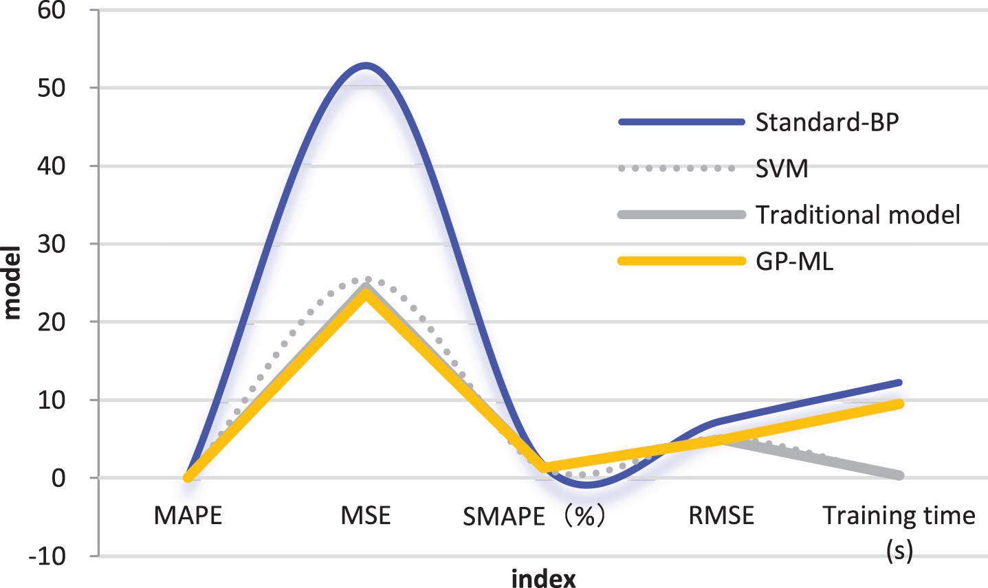
Statistical diagram of comparison results of different models.

Table 2 shows examples of data sets after pre-processing and normalization.

Table 2

Examples of normalized data sets

ht -1	ht-2	ht-3	jt-1	jt-2	jt-3	ft-1	ft-2	ft-3	wt-1
0.501	0.561	0.512	0.794	0.836	0.75	0.139	0.122	0.104	0.875
0.521	0.501	0.561	0.787	0.794	0.836	0.144	0.139	0.122	0.781
0.541	0.521	0.501	0.795	0.787	0.794	0.112	0.144	0.139	0.853
...	... .	...	...	...	...	...	...	...	...
wt-2	wt-3	xt-1	xt-2	xt-3	Δft-1	Δft-2	day of week	time of week	ft
0.803	0.813	0.756	0.639	0.634	0.566	0.567	0.55	0.1	0.144
0.875	0.803	0.715	0.756	0.639	0.555	0.566	0.55	0.103	0.112
0.781	0.875	0.738	0.715	0.756	0.521	0.555	0.106	0.109
...	... .	...	...	...	...	...	...	...	...

The comparison results of the models are shown in Table 3 and Fig. 4. It can be seen from the table that although the model proposed in this study is higher than the traditional model in training time, it is far better in other error performance indicators than the traditional model. The reason why the model proposed in this research is higher than the traditional model in training time is that the number of hidden layers and the number of neurons are higher than the traditional model, which causes a large amount of calculation. Therefore, the results prove the powerful computing and modeling capabilities of the model proposed in this study. Moreover, the error of the performance index of the model in this study is small, which also proves the good prediction accuracy and convergence of the model proposed in this study to a certain extent. Through the above comparative analysis, it can be seen that the model proposed in this study is superior to the traditional model in processing large-scale data sets, which verifies the advantages of the model proposed in this study when processing large-scale data sets.

Table 3

Statistical table of performance comparison of large-scale data sets

Indicator Model	Traditional model	GP-ML
MAPE	0.2148	0.0942
MSE	79.03	31.03
SMAPE (%)	4.044	2.21
RMSE	8.89	5.57
Training time (s)	23.68	100.63

Fig. 4

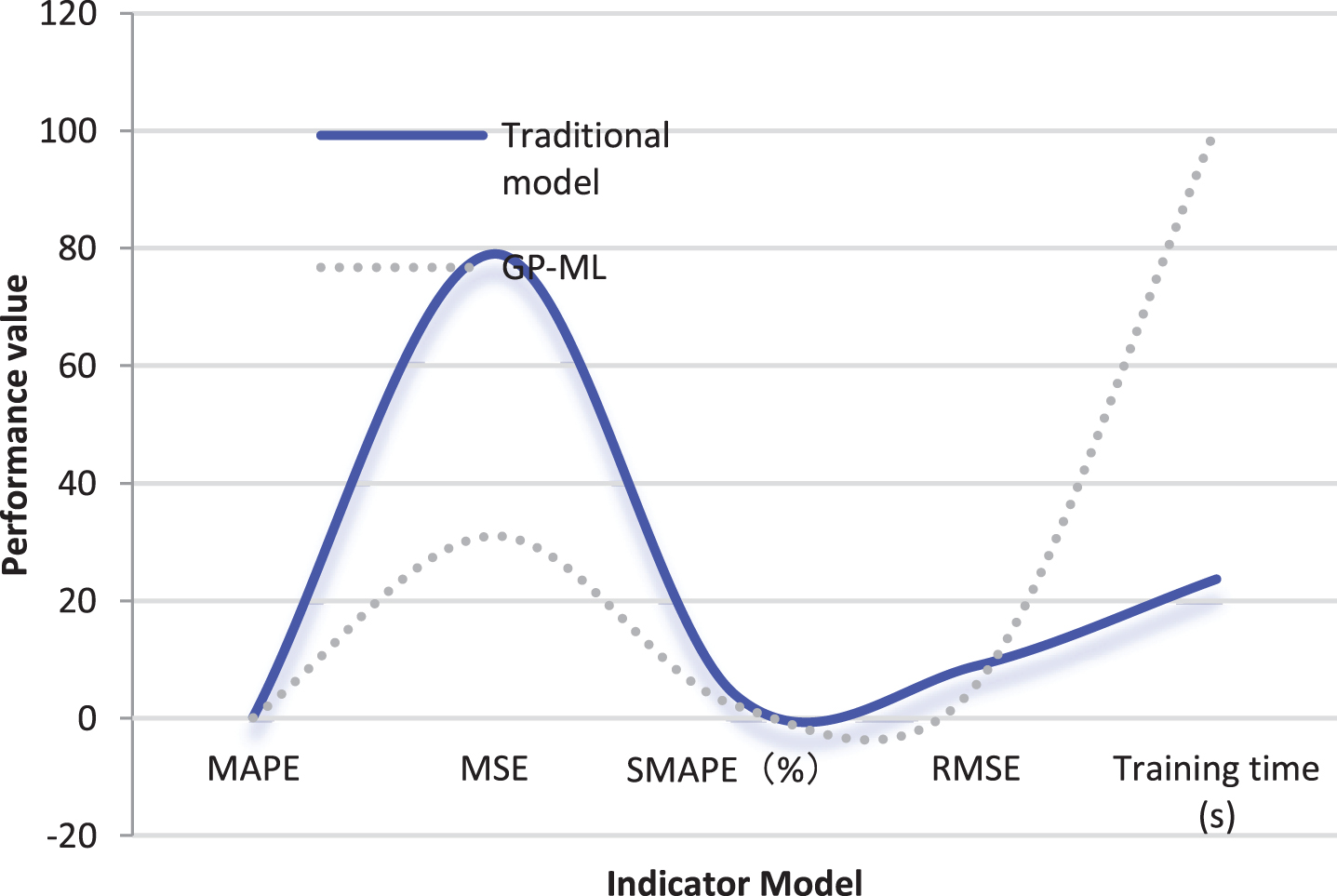
Statistical diagram of performance comparison of large-scale data sets.

In order to further study the performance of the model proposed in this study, this study studies the evaluation effect of the model on teaching quality. The quality of online English teaching and traditional classroom English teaching is evaluated by manual and the model proposed in this study. There are 30 groups of comments. The results obtained are shown in Tables 4, 5, Figs. 5 and 6.

Table 4

Statistics table of traditional classroom teaching quality evaluation

	Manual scoring	Model scoring		Manual scoring	Model scoring
1	73.7	70.7	16	80.4	86.2
2	69.5	72.9	17	72.2	70.5
3	64.3	61.9	18	67.0	79.6
4	68.9	57.3	19	78.7	64.8
5	66.0	59.9	20	63.7	53.7
6	71.5	83.8	21	73.5	61.3
7	69.7	71.1	22	75.4	65.5
8	68.1	56.0	23	70.5	69.6
9	66.9	54.7	24	62.2	64.2
10	77.9	65.4	25	64.7	67.0
11	62.1	62.7	26	69.0	67.1
12	70.2	59.2	27	68.6	75.4
13	68.5	70.2	28	70.4	75.1
14	79.2	83.5	29	70.8	59.5
15	80.3	90.6	30	71.6	79.3

Table 5

Statistical table of online classroom teaching quality evaluation

	Manual scoring	Model scoring		Manual scoring	Model scoring
1	77.1	74.1	16	69.9	81.9
2	71.6	71.4	17	68.2	71.2
3	79.4	72.0	18	73.0	81.6
4	70.4	64.9	19	66.9	70.7
5	67.8	56.7	20	71.3	59.9
6	80.8	93.7	21	81.6	94.6
7	72.8	86.8	22	64.9	58.2
8	74.9	63.6	23	68.8	74.0
9	66.3	54.9	24	66.6	69.7
10	63.4	68.8	25	70.3	83.5
11	79.4	84.1	26	73.1	66.5
12	71.6	77.8	27	66.8	74.0
13	81.0	86.9	28	73.4	82.0
14	77.4	89.7	29	63.4	66.7
15	81.6	93.9	30	70.8	78.7

Fig. 5

Statistical diagram of traditional classroom teaching quality evaluation.

Fig. 6

Statistical table of online classroom teaching quality evaluation.

It can be seen from Tables 4, 5, Figs 5 and 6 that the model proposed in this study has good performance in the evaluation of English teaching quality in traditional classrooms and online classrooms. This shows that the algorithm proposed in this paper has certain advantages and can be applied to the practice of English intelligent teaching system.

7 Conclusion

The evaluation of teaching quality in colleges and universities is an important link in the process of teaching management in colleges and universities. It requires many evaluation indexes and is affected by many factors, which makes the evaluation index and the result of teaching quality show a complex nonlinear relationship. This paper mainly studies the active learning algorithm for the problem that a large amount of data is easy to obtain but difficult to label in real life. Based on the relevance vector machine model, the active learning algorithm is studied. Moreover, the mixed Gaussian is used to explore the distribution characteristics of the samples, the classic relevance vector machine model is improved, and an active learning algorithm combining sparse Bayesian learning and mixed Gaussian is proposed In addition, this study strategically selects and labels samples, and constructs a classifier that combines the distribution characteristics of the samples, so as to reduce the number of labeling samples as much as possible while ensuring good prediction accuracy. In order to verify that the model proposed in this study has more advantages in evaluation of teaching quality than other shallow models, the parameters of this study model are optimized. Through comparative analysis, we can see that the model proposed in this study has good performance in the evaluation of English teaching quality in traditional classrooms and online classrooms. This shows that the algorithm proposed in this paper has certain advantages and can be applied to the practice of English intelligent teaching system.

References

Delgaty

Laura.

, Twelve tips for academic role and institutional change in distance learning, Medical Teacher 37(1) (2015), 41–46.

Stefanovic

, Tadic

, Nestic

, et al., An assessment of distance learning laboratory objectives for control engineering education, Computer Applications in Engineering Education 23(2) (2015), 191–202.

Remesh

Babu P.

, Developing open and distance learning programme in labour and development: results of a needs assessment study, Journal of Natural History 196(29) (2015), 265–291.

, Low

S.P.

, Liu

J.Y.

, et al., Critical success factors in distance learning construction programs at central Queensland University: Students’ perspective, Journal of Professional Issues in Engineering Education and Practice 141(1) (2015), 05014003.

Willis

E.A.

, Szabo-Reed

A.N.

, Ptomey

L.T.

, et al., Distance learning strategies for weight management utilizing social media: A comparison of phone conference call versus social media platform. Rationale and design for a randomized study, Contemporary Clinical Trials 47 (2016), 282–288.

H.J.

, Zhan

D.C.

and Jiang

, Fast generalization rates for distance metric learning: Improved theoretical analysis for smooth strongly convex distance metric learning, Machine Learning 108(2) (2019), 267–295.

Luo

, Wen

, Liu

, et al., Transferring knowledge fragments for learning distance metric from a heterogeneous domain, IEEE Transactions on Pattern Analysis and Machine Intelligence 41(4) (2019), 1013–1026.

Hsu

C.C.

, Kung

C.H.

, Jheng

J.J.

, et al., Unsupervised distance learning for extended self-organizing map and visualization of mixed-type data, Intelligent Data Analysis 23(4) (2019), 799–823.

Huang

Ning

, Analysis and design of university teaching evaluation system based on JSP platform, Journal of Education & Management Engineering 7(3) (2017), 43–50.

10.

Murcia

J.A.M.

, Torregrosa

Y.S.

and Belando

, Questionnaire evaluating teaching competencies in the university environment. Evaluation of teaching competencies in the university, Naer Journal of New Approaches in Educational Research 4(1) (2015), 54–61.

11.

Liu

and Chen

, Research on fuzzy comprehensive evaluation in practice teaching assessment of computer majors, International Journal of Modern Education & Computer Science 7(11) (2015), 12–19.

12.

Zhou

, Li

and Sun

, Teaching performance evaluation by means of a hierarchical multifactorial evaluation model based on type-2 fuzzy sets, Applied Intelligence 46(1) (2016), 1–11.

13.

Lalvarmawi

Florence

, Banik

Uttam

and Anita Devi

, Feedback of medical students on teaching and evaluation methodology in Physiology, National Journal of Physiology Pharmacy & Pharmacology 5(2) (2015), 102–113.

14.

Porozovs

, Liepniece

and Voita

, Evaluation of the teaching methods used in secondary school biology lessons, Nephron Clinical Practice 7(1) (2015), 60–66.

15.

Oliveros

María Amparo

, García

Alejandra

and Valdez

Benjamín

, Evaluation of a teaching sequence regarding science, technology and society values in higher education, Creative Education 6(16) (2015), 1768–1775.

16.

Cerón

Manuel Sánchez

and del Sagrario Corte Cruz

Francisca María

, The evaluation of teaching: some consequences for Latin America, Revista Mexicana De Investigacion Educativa 20(67) (2015), 1233–1253.

17.

Heitkamp

S.J

, Rüttermann

Stefan

and Gerhardt-Szép

Susanne

, Work shadowing in dental teaching practices: evaluation results of a collaborative study between university and general dental practices, Bmc Medical Education 18(1) (2018), 99–105.

18.

, Li

and Ge

, Application of data mining in the colleges’ in-class teaching quality evaluation system, Journal of Computers 10(3) (2015), 166–175.

19.

Wei

and Xin

Xiang-Yang

, Research evaluation on impact of mobile phone information technology on the urban public space development under the internet background, Journal of Intelligent & Fuzzy Systems 37(2) (2019), 1753–1759.

20.

Angell

and Tewell

, Teaching and un-teaching source evaluation: questioning authority in information literacy instruction, Communications in Information Literacy 11(1) (2017), 95–121.

21.

Brkovic

and Chiles

, ‘Spector –the sustainability inspector’: Participatory teaching, learning and evaluation game for architects, architecture students and pupils, Facta Universitatis 14(1) (2016), 1–20.

22.

, et al., A novel fingerprint feature extraction method for communication radiation source, Journal of Intelligent & Fuzzy Systems 37(1) (2019), 351–359.

23.

Reisenwitz

Timothy H.

, Student evaluation of teaching: an investigation of nonresponse bias in an online context, Journal of Marketing Education 38(4) (2015), 139–144.