Logistics engineering optimization based on machine learning and artificial intelligence technology

Abstract

In the era of the Internet of Things, smart logistics has become an important means to improve people’s life rhythm and quality of life. At present, some problems in logistics engineering have caused logistics efficiency to fail to meet people’s expected goals. Based on this, this paper proposes a logistics engineering optimization system based on machine learning and artificial intelligence technology. Moreover, based on the classifier chain and the combined classifier chain, this paper proposes an improved multi-label chain learning method for high-dimensional data. In addition, this study combines the actual needs of logistics transportation and the constraints of the logistics transportation process to use multi-objective optimization to optimize logistics engineering and output the optimal solution through an artificial intelligence model. In order to verify the effectiveness of the model, the performance of the method proposed in this paper is verified by designing a control experiment. The research results show that the logistics engineering optimization based on machine learning and artificial intelligence technology proposed in this paper has a certain practical effect.

Keywords

Machine learning artificial intelligence logistics optimization

1 Introduction

With the rapid development of information technology, the logistics industry is facing many challenges. Smartphones, social networks, tablets, global positioning systems, sensors, log files, and many other devices and sources generate large amounts of unstructured data every second. In addition, the amount of data generated each year is much larger than the previous amount of data, which is why our era is called the information age [1]. Data is the next hot spot in logistics informatization research. All these data contain valuable information, which can be used by the government and private companies to make in-depth predictions, analysis, and improve service quality of logistics data. Logistics companies must strive to seize the opportunities brought by the information age if they want to win initiative and achieve leapfrog development in the competition. The financial industry, institutions and academia have long been interested in the shipping industry. The Baltic Dry Index BDI (Baltic Dry Index), as a “barometer” for the shipping industry, has received widespread attention from economists and market investors. The international trade market is becoming more and more prosperous, which is also an intuitive reference material for investors, so the research on the shipping index is very meaningful. In addition, it combines the future economic activities and thus has the characteristics of leading economic indicators. The model input in previous studies usually includes price and quantity data, and may also include the selection of technical indicators, but few papers use basic indicators in the model. Compared with technical analysis, basic analysis focuses more on intuitive physical interpretation and attempts to find the intrinsic value of assets. The selected basic variables generally have a direct judgment on the information contained in the model and have a certain relationship with the goal. The logistics industry urgently needs effective data mining methods, and artificial intelligence has a great advanlabele as a classification tool because artificial intelligence is a new general-purpose learning machine developed on the basis of mature statistical theory. Artificial intelligence has proven to be a useful technique for data classification, regression and prediction. In pattern recognition or regression, artificial intelligence is clearly more prominent than other methods in terms of test set error rate. Although artificial intelligence methods have been widely used in index forecasting, almost no analysis has extended to the shipping market. However, transactions between international goods are more and more prosperous and frequent, and it is also one of the most important emerging markets in the world. Of course, the increase of data is a big problem that we need to face, so it is an inevitable trend to find effective ways to improve the ability of data mining algorithms to handle the increase in data [3].

2 Related works

The literature [4] used the Bender decomposition algorithm and the branch-and-bound method to solve the problem of facility location with unlimited storage capacity and believed that transportation distance and transportation cost are non-linear convex function relationship for facility location. In order to realize the overall optimization of the supply chain, the literature [5] constructed a mixed integer programming model that aimed at total cost and made optimal decisions about the layout of logistics facilities and the distribution of outlet demand. The literature [6] studied the general logistics facility location problem while considering the distribution vehicle path planning and established a bi-level planning model based on dynamic demand. Moreover, it compared the calculation results with the results solved by other methods. The results show that the accuracy of this method has been improved. When studying the location problem, literature [7] established a 0.1 integer nonlinear location model considering the discrete and random demand and the limited capacity of the distribution center, and transformed the nonlinear programming into linear programming, and used the meta-heuristic algorithm to solve the example model. The literature [8] studied the problem of location selection considering the maximum distance limit of facility coverage and constructed a mixed integer quadratic constraint model under the condition of a certain Euclidean distance. Moreover, it used a three-slabele heuristic algorithm to solve and concluded that the cost is greatly reduced when the distance limit is tight. The literature [9] studied the location of logistics facilities and decision-making of path planning for the common distribution mode under the horizontal cooperation of logistics enterprises, and further adjusted the level of cooperation between enterprises to obtain the distribution plan with the lowest total cost.

The early research on the location of logistics centers mainly analyzes the factors that affect the location decision, and then uses various fuzzy evaluation methods to make decisions on the plan. The literature [9] used heuristic algorithm to calculate the cost of each site selection scheme, screened out part of the scheme, and then used fuzzy theory to quantify each evaluation index, and further comprehensive evaluation and screening scheme to obtain the most optimal site results. The literature [10] considered the benefits of logistics planners and customers separately in the location selection decision, and also considered the impact of distribution paths on costs, established a two-level planning model, and proved the rationality of the model with examples. The literature [11] initially explored the location of urban underground logistics system nodes using a set-cover model, which added new ideas to the location problem solving. The literature [12] proposed an interval decision model for continuous logistics facility location based on the center of gravity method and studied the logistics system planning problem with uncertain demand. Based on a new cuckoo algorithm, the literature [13] studied the location of e-commerce logistics center and used Levi’s flight mechanism to conduct a series of simulation experiments to study the location problem of railway logistics center. Moreover, it built a model based on demand coverage and transportation costs, used ILOGCPLEX software to solve it, and verified the effectiveness of the model with case results. In view of the characteristics of logistics distribution facility location problem, literature [14] designed a set of logistics facility location method with the idea of BIRCH clustering. This method combines the BIRCH clustering algorithm and the center of gravity method based on Dijkstra distance, and provides a new method to solve the problem of logistics facility location.

Foreign studies on LRP issues are relatively early and relatively mature. In the 1960s, some foreign scholars had already proposed some similar concepts, and linked site selection and transportation issues together. The literature [15] considered the influence of transportation paths and the characteristics of VRP distribution order when solving the location problem and designed a double-layer LRP model for blood bank location and transportation path planning, which symbolized the birth of LRP theory in the true sense. After that, the LRP model is solved separately, the initial solution is randomly generated first, and the tabu search algorithm is used to solve the LAP and VRP problems. Considering the dynamics of customer demand, a dynamic model of LRP based on customer demand was established. The literature [16] applied the LRP model to the field of communication. As the research on the LRP problem becomes more and more mature, scholars have focused more on the selection and improvement of algorithms. The literature [17] constructed a dual-target multi-site LRP mathematical model and used the multi-target subspace search (MOSS) algorithm to solve. Moreover, it compared the running results and efficiency of the algorithm and elite tabu search (ETS) and studied the LRP problem considering environmental factors. In addition, when establishing the model, it taken the minimum operating cost and the minimum environmental impact as dual goals, and further explored the impact of carbon emissions on the problem results. The literature [18] studied the LRP problem under the supplier-managed inventory model, built a model with the objective of optimizing the overall cost of the supply chain, and designed an improved genetic algorithm to further study the impact of vehicle capacity on the total cost of the supply chain.

The literature [19] studied the problem of site selection and transportation from an integrated perspective, which only aroused widespread concern in the domestic academic community on the issue of LRP. Moreover, it constructed a multi-objective LRP integer programming model that is more in line with urban distribution, divided the solution process into two slabeles, and uses heuristic search algorithms to complete the solution. The literature [20] established a multi-objective LRP model with the optimization objectives of shortening the multi-slabele response cycle and cost of logistics to study the influence of variables selected by different transportation modes on the results[21 –23]. Considering the time constraints required by customers in the study of LRP, in the case of multiple logistics facilities and multiple vehicle models[24 –29], In this study, an LRP model for simultaneous delivery and pickup based on fuzzy time windows was established, and the model was solved using a combination of an improved simulated annealing algorithm and a two-slabele adaptive genetic algorithm. Moreover, in this study, with the background of emergency rescue, a single-slabele emergency LRP model is constructed, and the improved bat algorithm is used to solve, and the optimal path arrangement of the problem is obtained.

3 Research on multi-label classification theory

The multi-label learning framework considers the situation where an object is associated with multiple labels, and there are certain differences from the traditional supervised learning framework. Therefore, the sample in multi-label learning is composed of one sample and corresponding multiple labels. The purpose of multi-label learning is to assign multiple appropriate labels to unknown samples. x = R^d is assumed to represent a d-dimensional sample space, and L ={ l₁, l₂, ⋯ , l_m } represents a label space containing m categories. A multi-label training set D ={ (x_i, y_i) |i = 1, 2, ⋯ , n } with n samples is given. Among them, x_i represents the feature vector of the i-th sample, y_i ⊆ L is the label set of the i-th sample, and the task of the learning system is to learn a multi-label classifier from it h : x → 2^y. Based on this, for any sample x ⊆ X, the classifier predicts that the set of class labels belonging to that sample is h (x) ⊆ y.

The main idea of the multi-label classification method based on problem conversion is to convert the multi-label classification problem into multiple single-label classification problems, and then use the proposed single-label classification method to train and learn the multi-label classification problem. At present, the existing mature single-label learning methods mainly include first-order methods BR and CC, second-order methods RPC and CLR, and higher-order methods LP, PPT and RAkEL.

(1) Binary Relation Method

The basic idea of the BR method in solving the multi-label learning problem is to convert the multi-label learning problem into m separate binary classification problems, where each binary classification problem corresponds to a category label in the label space χ.

The BR method generates a separate data set for each label l_i, and a total of m data sets D_{l
_i} (i = 1, 2, ⋯ , m) are generated. Each data set contains all training samples in the training set. The samples in each data set are the same, the only difference is that each sample corresponding labels are different. For the data set D_{l
_i}, all the samples contained in the data set are only marked whether they belong to the label l_i, and the data set is used to train a binary classifier that only outputs whether the samples belong to the label l_i, thus training a corresponding for each label second classifier. For the predicted samples, the final classification results are obtained after reasonable integration of the classification results of all binary classifiers in some way.

(2) Classified Chain

On the basis of the BR method, BR does not consider the correlation between the labels at all, so the BR is improved, the CC classifier chain method is proposed, and the ECC (Ensemble Classified Chains) combined classifier chain method is further proposed.

(3) Ranking by Pairwise Comparison

The RPC method generates a data set for each pair of markers (l_i, l_j) (1 ⩽ i ⩽ j ⩽ m). This dataset only selects the samples marked by one of the pair of markers (excluding the samples marked by these two markers at the same time), and a total of $G_{n}^{2}$ will be generated data sets. Each data set is used to train a binary classifier (because each classifier only needs to deal with (- l_i, l_j) and (l_i, - l_j) cases). When predicting an unknown sample, all the two classifiers are activated, and through the “committee voting mechanism”, all the labels related to the sample are ranked according to the number of votes obtained for each label.

(4) Calibrated Label Ranking

The CLR (Calivrated Label Ranking) calibrated label ranking method is an extension method based on the RPC method. This method adds an artificial calibration label on the basis of RPC and uses the label as a set of related and unrelated marks in the set of marks split point. Since the calibration mark is a mark added manually, in the combination with the original mark, each training sample is a positive example for its related mark and negative for the calibration mark. At the same time, it is a negative for its unrelated mark example, and for the calibration mark is a positive example.

(5) Label Powerset

The main idea of this method is to regard the label set Y_i to which each sample belongs as a whole single label l_{Y
_i}, and all the label combinations l_{Y
_i} with different values appearing in the training set data form a single label set l_Y, so that multi-label learning problem is flexibly transformed into a new single-label learning problem.

(6) Pruned Problem Transformation

PPT (Pruned Problem Transformation) is a modification of the LP method by pruning. This method removes the label combination whose frequency of occurrence in each subset is less than a predetermined threshold by pruning technology. This reduces the possibility of data skew caused by new labels containing too few samples generated by the LP method.

(7) Random k-Labelsets

RAkEL (Random k-1abelsets) is an improvement to the LP method and a combination of the LP methods. This method is mainly to randomly generate a subset of markers in the combination of markers, and then use the LP method to perform multi-label classification in each marker subset. The RAkEL method fully considers the correlation between the labels, and also reduces the possibility that the LP method may produce skewed data. However, in order to achieve near-optimal performance in the RAkEL method, the input parameters such as: subset size, the number of models, thresholds, etc. are internally cross-checked, and it is difficult to find the optimal parameters when the training samples are insufficient.

Multi-label learning method based on DT (Decision Tree) is a more reliable multi-label learning method. C4.5 is a commonly used single-label classification method with good classification effect. On this basis, Clare and King Scholars and other scholars have proposed improvements to this method. In the improved decision tree method, leaf nodes are allowed to be a set of labels, and the corresponding information entropy calculation formula is modified. The modified information entropy formula is as follows: $\begin{matrix} Entropy (D) = \\ - \sum_{j = 1}^{m} (p (l_{j}) log p (l_{j}) + q (l_{j}) log q (l_{j})) \end{matrix}$ (1)

In the formula, p (l_j) is the probability (correlation probability) belonging to the label l_j, q (l_j) = 1 - p (l_j).

4 Multi-mark classification evaluation index

For the multi-label learning problem, each sample object may have multiple labels at the same time, so the evaluation of the classification effect of the multi-label classifier becomes more complicated than that of the single-label classifier. It is not possible to directly use single mark to evaluate index accuracy, precision rate and recall rate. To this end, researchers have successively proposed multiple evaluation indicators suitable for multi-label classification problems based on single-label classification evaluation indicators, which are generally divided into two types: classification-based evaluation indicators and ranking-based evaluation indicators. In the following description, (x_i, y_i) (i = 1, 2, ⋯ , n) is used to represent the samples in the test set, among them, x_i represents the feature vector of the i-th sample, and y_i ⊆ L is the label set of the i-th sample. For a sample x_i, Z_i is used to represent the set of labels that x_i belongs to as predicted by the multi-label classifier, and r_i (l) represents the ranking of label 1 in sample x_i among all labels.

The classification-based evaluation indicators can be further subdivided into sample-based evaluation indicators and marker-based evaluation indicators according to different considerations. The difference between the two types of evaluation indicators is that the evaluation indicators based on the sample are the average of the differences between the prediction results of all samples in the test set and the real situation. However, the marker-based evaluation index is measured by predicting the results of each individual marker, and finally averaging the results of all markers.

(1) Evaluation indicators based on examples

1. Hamming loss ${hloss}_{χ} (h) = \frac{1}{n} \sum_{i = 1}^{n} \frac{1}{m} | Z_{i} Δ Y_{i} |$ (2)

The evaluation index expresses the performance of the multi-label classifier by calculating the degree of difference between the label result predicted by the multi-label classifier and the label contained in the actual sample. This indicator mainly examines the misclassification of a sample on a single mark, that is, the probability that a mark that actually belongs to the sample does not appear in the mark set, but a mark that does not belong to the sample appears in the mark set. Therefore, the smaller the value, the better the classification effect of the learning system. Among them, operator Δ is used to measure the “symmetric difference” between the two sets, and operator | · | is used to return the “potential” of the set.

2. Accuracy ${acc}_{χ} (h) = \frac{1}{n} \sum_{i = 1}^{n} \frac{Z_{i} \cap Y_{i}}{Z_{i} \cup Y_{i}}$ (3)

Accuracy classification accuracy is one of the most intuitive evaluation methods, which requires that the prediction mark must be completely consistent with the actual mark, which does not include part of the correct situation.

3. Precision ${pre}_{χ} (h) = \frac{1}{n} \sum_{i = 1}^{n} \frac{| Z_{i} \cap Y_{i} |}{| Z_{i} |}$ (4)

The percenlabele of the predicted class labels that are the same as the class labels in the predicted class labels.

4. Recall ${recall}_{χ} (h) = \frac{1}{n} \sum_{i = 1}^{n} \frac{| Z_{i} \cap Y_{i} |}{| Y_{i} |}$ (5)

The percentage of the actual predicted tags with the actual class tags of the text.

5. F_1-score $F_{1} - {score}_{χ} (h) = \frac{1}{n} \sum_{i = 1}^{n} \frac{2 | Z_{i} \cap Y_{i} |}{| Z_{i} | + | Y_{i} |}$ (6)

Multi-label classification evaluation often seeks to balance between recall and precision. F-score is a commonly used balance method, defined as the harmonic mean of recall and precision.

6. Subset accuracy ${subsetacc}_{χ} (h) = \frac{1}{n} \sum_{i = 1}^{n} [[Z_{i} - Y_{i}]]$ (7)

The evaluation index is used to investigate the proportion of samples in the test set that the predicted label set and the real set exactly match. The larger the value of this index, the better the system performance. When the value is 1, the system performance is the best.

(2) Mark-based evaluation indicators

Unlike the evaluation index based on the sample, the evaluation index based on the mark is decomposed into a separate measurement of each mark in the mark set. It measures the classification effect of the learning system on a single mark,and the final result is that it is in all the marks “Macro-/micro-averaged value” on the page. Specifically, for a certain label l_j in the label set, the classification performance of the learning system at l_j is usually measured by the following four indicators:

TP_j (true positive instances): The number of real cases in the prediction result set: ${TP}_{j} = | {x_{i} | l_{j} \in Y_{i} \land l_{j} \in h (x_{i}), (x_{i}, Y_{i}) \in D} |$ (8)

FP_j (false positive instances): Number of false positives in the prediction result set: ${FP}_{j} = | {x_{i} | l_{j} \notin Y_{i} \land l_{j} \in h (x_{i}), (x_{i}, Y_{i}) \in D} |$ (9)

TN_j (true negative instances): The number of true and negative examples in the prediction result set: ${TN}_{j} = | {x_{i} | l_{j} \notin Y_{i} \land l_{j} \notin h (x_{i}), (x_{i}, Y_{i}) \in D} |$ (10)

FN_j (true positive instances): Number of false negative examples in the prediction result set: ${FN}_{j} = | {x_{i} | l_{j} \in Y_{i} \land l_{j} \notin h (x_{i}), (x_{i}, Y_{i}) \in D} |$ (11)

As can be seen from the above formula, TP_j + FP_j + TN_j + FN_j = n, it can be seen that the commonly used two-class performance indicators can be calculated by the above four statistics, for example: $\begin{matrix} Accuracy = B_{a} ({TP}_{j}, {FP}_{j}, {TN}_{j}, {FN}_{j}) \\ = \frac{{TP}_{j} + {TN}_{j}}{{TP}_{j} + {FP}_{j} + {TN}_{j} + {FN}_{j}} \end{matrix}$ (12)

$Precision = B_{p} ({TP}_{j}, {FP}_{j}, {TN}_{j}, {FN}_{j}) = \frac{{TP}_{j}}{{TP}_{j} + {FP}_{j}}$ (13)

$Recall = B_{r} ({TP}_{j}, {FP}_{j}, {TN}_{j}, {FN}_{j}) = \frac{{TP}_{j}}{{TP}_{j} + {FN}_{j}}$ (14)

1. Macro precision $Macroprecision = \frac{1}{m} \sum_{j = 1}^{m} B_{p} ({TP}_{j}, {FP}_{j}, {TN}_{j}, {FN}_{j})$ (15)

2. Macro recall $Macrorecall = \frac{1}{m} \sum_{j = 1}^{m} B_{r} ({TP}_{j}, {FP}_{j}, {TN}_{j}, {FN}_{j})$ (16)

3. Macro F₁ $Micro_F_{1 χ} (h) = \frac{1}{m} \sum_{j = 1}^{m} F_{1 j}$ (17)

4. Micro precision $\begin{matrix} Microprecision = \\ B_{p} (\sum_{j = 1}^{m} {TP}_{j}, \sum_{j = 1}^{m} {FP}_{j}, \sum_{j = 1}^{m} {TN}_{j}, \sum_{j = 1}^{m} {FN}_{j}) \end{matrix}$ (18)

5. Micro recall $\begin{matrix} Microrecall = \\ B_{r} (\sum_{j = 1}^{m} {TP}_{j}, \sum_{j = 1}^{m} {FP}_{j}, \sum_{j = 1}^{m} {TN}_{j}, \sum_{j = 1}^{m} {FN}_{j}) \end{matrix}$ (19)

6. Micro F₁ $Micro_F_{1 χ} (h) = \frac{2 (P * R)}{P + R}$ (20)

Among them, P is micro precison, R is micro recall, and F₁ is the harmonic mean of precision and recall rate.

The focus of multi-mark classification evaluation indicators based on ranking is the correctness of the ranking of each mark in the mark set corresponding to the sample.

1. one error $one - {error}_{χ} = \frac{1}{n} \sum_{i = 1}^{n} | {arg min_{l \in Y_{i}} r_{i} (l) \in Y_{i}} |$ (21)

This indicator examines the probability that the first label in the ranking of predicted labels does not belong to the sample-related label set. The smaller the index value is, the higher the performance is, and when one - error = 0, the performance is the best.

2. Coverage ${coverage}_{χ} (h) = \frac{1}{n} \sum_{i = 1}^{n} max_{l \in Y_{i}} r_{i} (l_{i}) - 1$ (22)

This indicator calculates the farthest position in the ranking of prediction marks among all the related marks of each sample. The smaller the coverage value, the better the performance.

3. Ranking loss

$\begin{matrix} {rankingloss}_{χ} (h) = \\ \frac{1}{n} \sum_{i = 1}^{n} \frac{1}{| Y_{i} | | {\bar{Y}}_{i} |} | {(l_{a}, l_{b}) : r_{i} (l_{a}) > r_{i} (l_{b}), (l_{a}, l_{b}) \in Y_{i} \times \bar{Y}} | \end{matrix}$ (23)

This indicator detects the average probability of irrelevant labels ranking in front of the relevant labels in the order of predicted labels of all samples. The smaller the index value, the better the performance. When rankingloss = 0, the performance is the best.

4. Average precision

${avgprec}_{χ} (h) = \frac{1}{n} \sum_{i = 1}^{n} \frac{1}{| Y_{i} |} \sum_{l \in Y_{i}} \frac{| l^{'} \in Y_{i} : r_{i} (l^{'}) ⩽ r_{i} (l) |}{r_{i} (l)}$ (24)

This indicator mainly examines the ranking results of the predicted labels in all samples, which is ranked in front of the relevant labels and is also the average value of the probability of the relevant labels.The larger the value, the better the performance. When averageprecision = 1, the performance is the best.

5 Logistics engineering optimization

(1) Two-point crossing between paths: An element on the two sub-paths is selected, deleted from the original path, and inserted into the other sub-path. Before inserting, it is first determined the m customers closest to the current element to be inserted, and it is determined whether there is at least one customer of n customers in another sub-path. If it exists, it is selected to insert the new path with the smallest total distribution cost, otherwise it is not inserted. The specific content is shown in Fig. 1.

Fig. 1

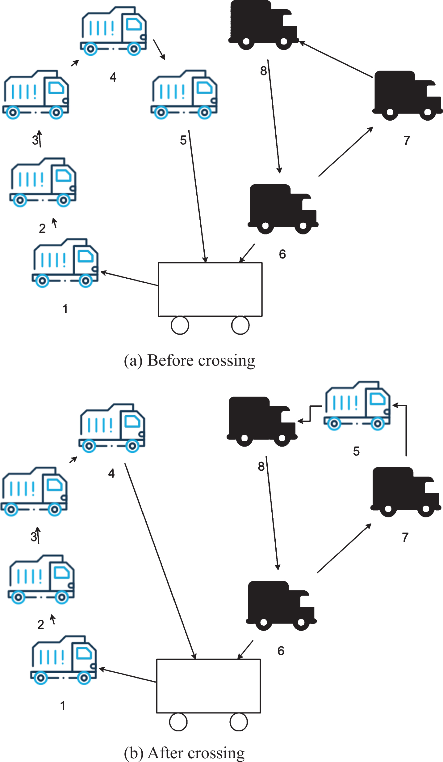
Two-point crossing between paths.

Single-point transfer between paths: Two paths in an existing path are randomly selected, and a customer point on one of the paths is deleted from the path, and the customer point is placed on the second path. The place where it can be placed is the place with the lowest cost on the second path. The specific content is shown in Fig. 2.

Fig. 2

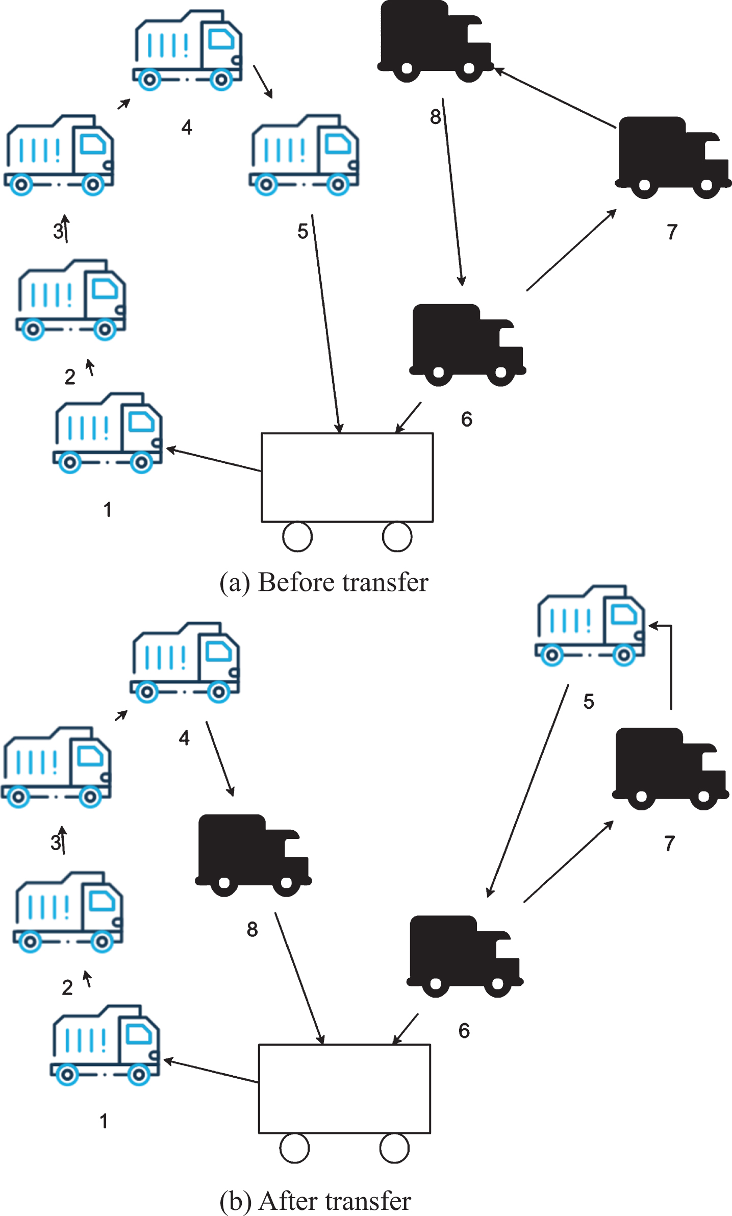
Single-point transfer between paths.

Two points exchange between paths: One of the existing paths is randomly selected, and two customer points are selected on this path, so that the positions of the two customer points are swapped to obtain a new path. The cost of the new path is smaller than the original path. The specific content is shown in Fig. 3.

Fig. 3

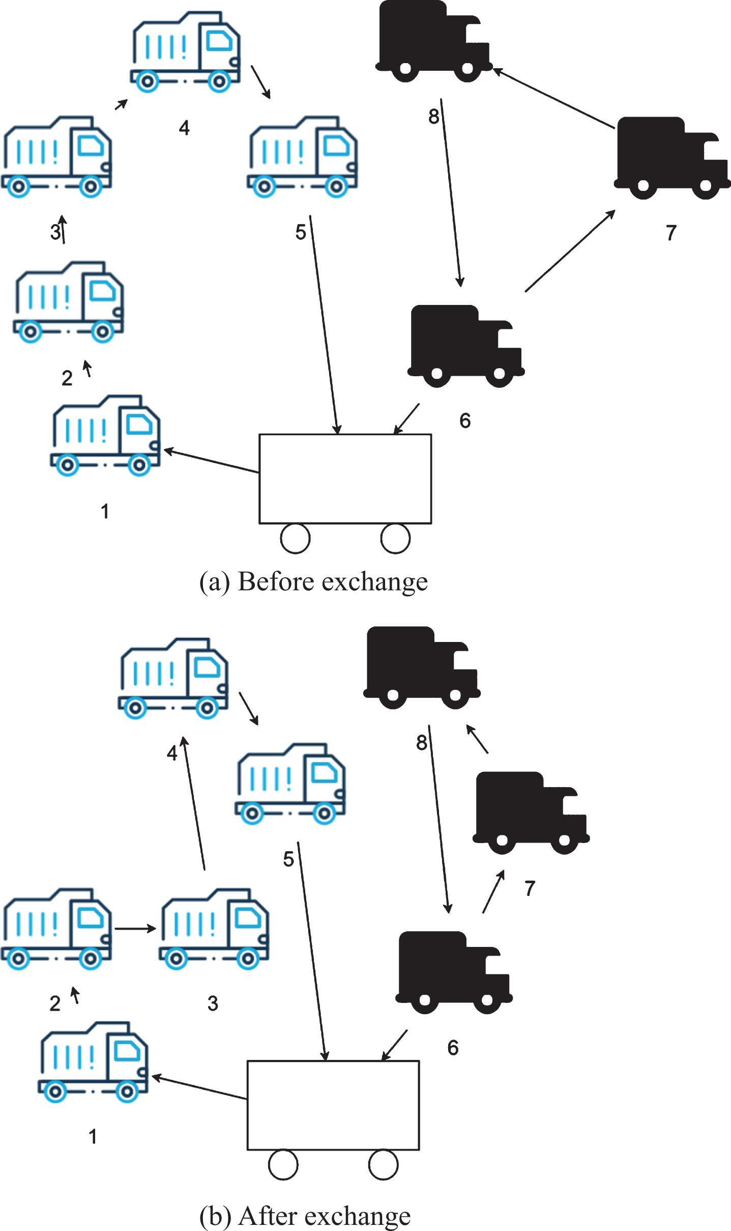
Two-point exchange in the path.

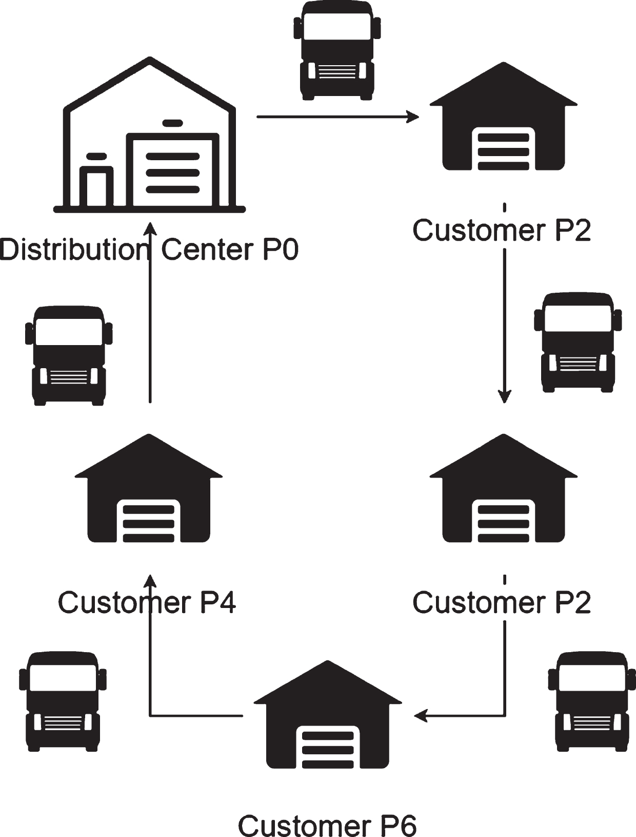
Path reversal: For the already planned path, the direction of vehicle travel is changed from front to back to back to front. The needs of each customer on this path can still be met. The average load rate of the vehicle may change, or the time the vehicle arrives at each customer point is different, resulting in a change in the total distribution cost, laying the foundation for iterative optimization. The specific content is shown in Fig. 4. Vehicle 1 transportation path as show in Fig. 5, Vehicle 2 transportation path as show in Fig. 6, Vehicle 3 transportation path as show in Fig. 7.

Fig. 4

Path reversal.

Fig. 5

Vehicle 1 transportation path.

Fig. 6

Vehicle 2 transportation path.

Fig. 7

Vehicle 3 transportation path.

Next, we conduct a case study. There are 7 transport vehicles with a load capacity of 8T in a logistics company, and the transported goods are transported to the hands of 8 customers. The customer numbers are 1–8, and the customer locations are all located in Kunming City. We set the delivery volume to be expressed in D_i, the recovered volume to be expressed in P_i, the unloading time to be expressed in T_i, and the time range to reach each customer point is between [ET_i, LT_i]. For the convenience of research, it is assumed that all customer requirements are reached after 13:00, and the relevant data is shown in Table 1. The distance from the distribution center to each customer point is shown in Table 2.

Table 1

Data table of service requirements of various customer points

Clienti	1	2	3	4	5	6	7	8
D_i	2.50	1.50	3.00	3.50	4.00	2.00	3.00	2.00
P_i	0.50	1.00	2.00	3.00	1.50	3.50	3.00	1.00
P_i -D_i	–2.00	–0.50	–1.00	–0.50	–2.50	2.50	0.00	–1.00
[ET_i, LT_i]	[1.50_i, 4.50]	[1.00_i, 2.00]	[1.00_i, 6.00]	[3.00_i, 5.00]	[5.00_i, 8.00]	[2.00_i, 4.50]	[2.00_i, 5.00]	[2.50_i, 8.00]
T_i	1.00	0.50	1.50	2.00	0.80	0.60	0.50	2.20

Table 2

Distance from distribution center to each customer point (km)

j ∖i	delivery center	1	2	3	4	5	6	7	8
0	0.0	35.0	65.0	70.0	100.0	250.0	208.0	250.0	90.0
1	35.0	0.0	70.0	40.0	105.0	220.0	80.0	123.0	110.0
2	65.0	70.0	0.0	65.0	90.0	200.0	85.0	130.0	90.0
3	70.0	40.0	65.0	0.0	95.0	200.0	85.0	130.0	90.0
4	100.0	105.0	90.0	95.0	0.0	190.0	80.0	132.0	100.0
5	250.0	220.0	200.0	185.0	190.0	0.0	150.0	125.0	164.0
6	108.0	80.0	85.0	110.0	80.0	150.0	0.0	122.0	90.0
7	150.0	123.0	130.0	135.0	132.0	125.0	122.0	0.0	100.0
8	90.0	110.0	90.0	120.0	100.0	164.0	100.0	100.0	0.0

It can be seen from the above table that the matrix is symmetrical. If a single line appears in the transportation process, the distance between the connecting points will be different, which is an asymmetric matrix. If it is assumed that the speed of the vehicle during driving is 45 km/h, the driving time is proportional to the situational distance. The time spent by the vehicle from i to j is t_ij = d_ij/45. The actual transportation process is affected by various factors. There are differences in the driving speed of different road sections, so it can be calculated separately.

First, we assume that the time from the distribution center P₀ to each customer point is s_i, the travel time is t_0i, and the customer time window constraint is [ET_i, LT_i]. After that, we calculate t₀ and the results are shown in Table 3.

Table 3

Travel time from distribution center P₀ to each customer point (h)

t₀₁	t₀₂	t₀₃	t₀₄	t₀₅	t₀₆	t₀₇	t₀₈
0.80	1.40	1.60	2.20	5.60	3.30	4.40	2.0

If t₀₁ < ET₁, s_i = ET₁, and If ET≤t₀₁≤LT₁, s_i = t₀₁. The initial value of s_i is shown in Table 4.

Table 4

Initial table from the distribution center to each customer time point s_i

s₁	s₂	s₃	s₄	s₅	s₆	s₇	s₈
1.50	1.40	1.60	3.0	5.60	3.30	4.40	2.50

Saving values from i to j: ΔL(i,j) = L_0i+L_0j-L_ij is calculated, and the calculated results are sorted. Since the two points of data in this case are symmetric, ΔL(i,j) =ΔL(j, i), the results are shown in Table 5.

Table 5

Distance saving scale between customer points

L(i,j)	(5,6)	(5,7)	(5,8)	(4,5)	(7,8)	(6,7)	(3,5)
ΔL(i,j)	275.0	208.0	176.0	160.0	140.0	136.0	135.0
L(i,j)	(4,6)	(4,7)	(2,5)	(6,8)	(4,8)	(2,6)	(2,7)
ΔL(i,j)	128.0	118.0	115.0	108.0	90.0	88.0	85.0
L(i,j)	(3,7)	(2,4)	(3,4)	(2,3)	(3,6)	(1,3)	(1,5)
ΔL(i,j)	85.0	75.0	75.0	70.0	68.0	65.0	65.0
L(i,j)	(2,8)	(1,6)	(1,7)	(3,8)	(1,2)	(1,4)	(1,8)
ΔL(i,j)	65.0	63.0	62.0	40.0	30.0	30.0	16.0

It is checked whether the two points can be effectively connected. If the (i, j) points are non-path points, they cannot be effectively connected. Then, it is checked whether (j, i) can be effectively connected. The results are shown in Table 6. The results are shown in Table 6.

Table 6

Verification table for point pairs (partial)

1	2	3	4	5	6	7
(i, j)	i, jLocation	Vehicle load at various points	EH_j=s_i+t_ij+T_i-s_j	ΔJorΔj	Whether to connect	S_r=s_r+EH_j
(5, 7).	Non-route points	Q₀ = 4 + 3≤8; Q₅ = 7-4 + 1.5≤8; Q₇ = 4.5-3 + 3≤8	EH₇ = s₅ + t₅₇ + T₅-s₇ = 4.8	Δj=0.6	No
(7, 5).	Non-route points	Q₀ = 4 + 3≤8; Q₅ = 7-4 + 1.5≤8; Q₇ = 4.5-3 + 3≤8	EH₇ = s₇ + t₇₅ + T₇-s₅ = 2.1	Δj=2.4	Yes	S₅ = s₅ ₊ EH₅ = 7.7
... ... .	... ... .	... ... .	... ... .	... ... .	... ... .	... ... .

After simplified by the above analysis, 8 customers can be delivered, and the final path is simplified to 3 paths, and the delivery can be completed by dispatching 3 vehicles.

Vehicle 1: It starts from the distribution center and loads goods of customer P₇ and customer P₅. It first travels from the distribution center to customer P₇. After arriving at customer P₇ to unload its goods, it travels from customer P₇ to customer P₅. After arriving at customer P₅ to unload its goods, it will be driven back by customer P₅ to the customer distribution center, thus forming a circular transportation path.

Vehicle 2: It starts from the distribution center and loads goods of customers P₂, P₆, P₄. It first travels from the distribution center to customer P₂. After arriving at customer P₂ to unload its goods, it travels from customer P₂ to customer P₆. After arriving at customer P₆ to unload its goods, it travels from customer P₆ to customer P₄. After arriving at customer P₄ to unload its goods, it will be driven back by customer P₄ to the customer distribution center, thus forming a circular transportation route.

Vehicle 3: It starts from the distribution center and loads the goods of customers P₁, P₂, P₈. It first travels from the distribution center to customer P₁. After arriving at customer P1 to unload its goods, it travels from customer P₁ to customer P₃. After arriving at customer P₃ to unload its goods, it travels from customer P₃ to customer P8. After arriving at customer P₈ to unload its goods, it will be driven back by customer P₈ to the customer distribution center, thus forming a circular transportation route.

Through the above analysis, we can see that the logistics engineering optimization based on machine learning and artificial intelligence technology proposed in this paper has certain practical effects.

6 Conclusion

Reducing the logistics cost of the distribution network and improving the overall efficiency and service quality of the distribution process are the basic directions of logistics development in the era of artificial intelligence. Based on the basic theoretical research of multi-label learning, for the instability of the classifier chain method and the combined classifier chain method and the problem of high algorithm complexity when processing high-dimensional data, a logistics engineering optimization system based on machine learning and artificial intelligence technology is constructed to enhance the learning ability of multi-label learning and improve the classification accuracy and efficiency of multi-label classification. For the problem that it is difficult to find a logistics expert that meets the demand under information overload, this study applies two improved multi-label chain learning methods RS-CC and RS-ECC for the recommendations of experts in the logistics field that it is a high-dimensional data problem. In order to further improve the reliability of the model in this paper, the performance of the method of the article is verified by designing a controlled experiment. From the research results, we can see that the logistics engineering optimization based on machine learning and artificial intelligence technology proposed in this paper has a certain practical effect.

Footnotes

Acknowledgment

This paper was supported by Nanjing Polytechnic Institute, Nanjing, Jiangsu, China, 1.“333 talents project”in Jiangsu Province; 2. “One hundred talents project” funding from college.

References

Speranza

M.G.

, Trends in transportation and logistics[J], European Journal of Operational Research 264(3) (2018), 830–836.

Savelsbergh

and Van Woensel

, 50th anniversary invited article—city logistics: Challenges and opportunities[J], Transportation Science 50(2) (2016), 579–590.

Hofmann

and Rüsch

, Industry 4.0 and the current status as well as future prospects on logistics[J], Computers in Industry 89 (2017), 23–34.

Govindan

, Soleimani

and Kannan

, Reverse logistics and closed-loop supply chain: A comprehensive review to explore the future[J], European Journal of Operational Research 240(3) (2015), 603–626.

Özdamar

and Ertem

M.A.

, Models, solutions and enabling technologies in humanitarian logistics[J], European Journal of Operational Research 244(1) (2015), 55–65.

Taniguchi

, Thompson

R.G.

and Yamada

, Recent trends and innovations in modelling city logistics[J], Procedia-Social and Behavioral Sciences 125(2014) (2014), 4–14.

Cattaruzza

, Absi

, Feillet

, et al., Vehicle routing problems for city logistics[J], EURO Journal on Transportation and Logistics 6(1) (2017), 51–79.

Zhong

R.Y.

, Huang

G.Q.

, Lan

, et al., A big data approach for logistics trajectory discovery from RFID-enabled production data[J], International Journal of Production Economics 165 (2015), 260–272.

Tofighi

, Torabi

S.A.

and Mansouri

S.A.

, Humanitarian logistics network design under mixed uncertainty[J], European Journal of Operational Research 250(1) (2016), 239–250.

10.

Abdulrahman

M.D.

, Gunasekaran

and Subramanian

, Critical barriers in implementing reverse logistics in the Chinese manufacturing sectors[J], International Journal of Production Economics 147 (2014), 460–471.

11.

Taniguchi

, Concepts of city logistics for sustainable and liveable cities[J], Procedia-Social and Behavioral Sciences 151 (2014), 310–317.

12.

Wang

, Gunasekaran

, Ngai

E.W.T.

, et al., Big data analytics in logistics and supply chain management: Certain investigations for research and applications[J], International Journal of Production Economics 176 (2016), 98–110.

13.

Grabara

, Kolcun

and Kot

, The role of information systems in transport logistics[J], International Journal of Education and Research 2(2) (2014), 1–8.

14.

Alshamsi

and Diabat

, A reverse logistics network design[J], Journal of Manufacturing Systems 37 (2015), 589–598.

15.

Bing

, Bloemhof

J.M.

, Ramos

T.R.P.

, et al., Research challenges in municipal solid waste logistics management[J], Waste Management 48 (2016), 584–592.

16.

Davarzani

, Fahimnia

, Bell

, et al., Greening ports and maritime logistics: A review[J], Transportation Research Part D: Transport and Environment 48 (2016), 473–487.

17.

Aljohani

and Thompson

R.G.

, Impacts of logistics sprawl on the urban environment and logistics: Taxonomy and review of literature[J], Journal of Transport Geography 57 (2016), 255–263.

18.

Schliwa

, Armitage

, Aziz

, et al., Sustainable city logistics—Making cargo cycles viable for urban freight transport[J], Research in Transportation Business & Management 15 (2015), 50–57.

19.

Lean

H.H.

, Huang

and Hong

, Logistics and economic development: Experience from China[J], Transport Policy 32 (2014), 96–104.

20.

Lagorio

, Pinto

and Golini

, Research in urban logistics: a systematic literature review[J], International Journal of Physical Distribution & Logistics Management, 2016.

21.

Boonmee

, Arimura

and Asada

, Facility location optimization model for emergency humanitarian logistics[J], International Journal of Disaster Risk Reduction 24 (2017), 485–498.

22.

Meidutė-Kavaliauskienė

, Aranskis

and Litvinenko

, Consumer satisfaction with the quality of logistics services[J], Procedia-Social and Behavioral Sciences 110 (2014), 330–340.

23.

Govindan

and Soleimani

, A review of reverse logistics and closed-loop supply chains: a Journal of Cleaner Production focus[J], Journal of Cleaner Production 142 (2017), 371–384.

24.

Carbone

, Rouquet

and Roussat

, The rise of crowd logistics: a new way to co-create logistics value[J], Journal of Business Logistics 38(4) (2017), 238–252.

25.

Kececioglu

O. Fatih.

, ‘Robust Control of High Gain DC-DC Converter Using Type-2 Fuzzy Neural Network Controller for MPPT’, Journal of Intelligent & Fuzzy Systems 37(1) (2019), 941–951.

26.

Volland

, Fügener

, Schoenfelder

, et al., Material logistics in hospitals: a literature review[J], Omega 69 (2017), 82–101.

27.

, Lei

S.P.

, Wang

Z.Z.

, et al., IoT-based real-time production logistics synchronization system under smart cloud manufacturing[J], The International Journal of Advanced Manufacturing Technology 84(1-4) (2016), 147–164.

28.

Mahajan

and Gupta

S.K.

, Methods to Solve QPPs with Fuzzy Parameters and Fuzzy Variables, Journal of Intelligent & Fuzzy Systems 37(2) (2019), 2757–2767.

29.

Boysen

, Emde

, Hoeck

, et al., Part logistics in the automotive industry: Decision problems, literature review and research agenda[J], European Journal of Operational Research 242(1) (2015), 107–120.