Interactive effects between monetary policy and fiscal policy based on dynamic stochastic general equilibrium model

1 Introduction

Monetary policy should not only exist as an economic policy, but also as a “public policy.” The People’s Bank of China is an important part of the government, and it is a public authority. Monetary policy has specific goals and guidelines and has a strong sense of orientation. Moreover, monetary policy is oriented toward the complex and changeable inflation and deflation issues. In addition, monetary policy affects the quality of life of the public and the well-being of society as a whole. Based on the above premise, we need a new public policy perspective to study monetary policy [1].

Generally speaking, monetary policy refers to the central bank’s use of various tools to adjust the money supply and interest rates in order to achieve established economic goals, thereby affecting the aggregate of macroeconomic policies and measures. At present, central banks of various countries always set interest rates and money supply as the intermediary targets of monetary policy, and take several or all of the indicators such as economic growth, full employment, price stability, balance of payments, and lower inflation rate as the ultimate goal of monetary policy. As the medium of monetary policy transmission, monetary policy tools are divided into general monetary policy tools and selective monetary policy tools. Among them, general monetary policy tools include three forms of legal deposit reserve ratio, rediscount rate and open market business. These three traditional monetary policy tools affect the entire macro-economy by regulating the total amount of money. Selective monetary policy tools include consumer credit control, securities market credit control, real estate credit control, preferential interest rates, and prepayment of import deposits. These monetary policy measures selectively regulate and influence credit in certain special areas. Monetary policy transmission mechanism refers to how monetary policy can use certain monetary policy tools to influence changes in the real economy and ultimately achieve the expected monetary policy goals. That is, the path that monetary policy needs to rely on to implement its impact. It is the basis for the effective functioning of monetary policy. Since the 1980s, the financial structure and economic environment of western industrialized countries have undergone major changes, and the transmission mechanism of monetary policy has also undergone significant changes [2].

Whether it is from the current status quo or the development trend, the development of the stock market has caused deep changes in my country’s financial structure and has affected my country’s monetary policy from different levels and degrees. It broadens the scope of the monetary policy, which leads to the diversification of the targets of monetary policy and the complexity of the implementation process. In this context, what kind of adjustments should be made to my country’s monetary policy to improve the effect of the policy is also worth studying. On the other hand, for investors in the stock market, if they want to grasp the laws of the market, make a reasonable investment portfolio, bear less risk, and obtain higher returns, they should identify all kinds of information that may affect the market and accurately predict the impact of monetary policy. Therefore, studying the effect of monetary policy in the stock market will also help investors in the stock market to correctly understand the impact of monetary policy on the market, reduce market volatility, and improve the efficiency of the stock market. In short, studying the relationship between the development of the stock market and monetary policy is not only a need for theoretical research, but also a practical topic on how to improve my country’s monetary policy [3].

2 Related work

The literature [4] believed that the change in money supply leads the S&P index. However, because money supply and demand are essentially endogenous variables, they cannot be simply measured by money stock, which makes people question the conclusions drawn by simple regression analysis methods. With the development of econometric research methods, economists began to use event research methods and vector autoregressive analysis methods (VAR models) to solve the endogenous problem of monetary supply.

The literature [5] used money supply as a measurement indicator and found that there is a reverse relationship between money supply changes and stock market price changes. The literature [6] took M1 as the research object and distinguished between expected and unexpected changes in the money supply, and mainly studied the unexpected money supply. Meanwhile, it is found that unexpected changes in money supply are inversely proportional to changes in stock market prices. In addition, some early empirical studies chose to use the discount rate as a measure of monetary policy. The literature [7] found that both technical and non-technical discount rate changes have a significant impact on stock prices, but non-technical discount rate changes have a stronger impact. Moreover, in their subsequent research, they examined the changes in the long-term return before and after the discount rate change and observed the impact of the discount rate change on the return before, during, and after the announcement. The conclusion is that in the three time periods, changes in the discount rate have an adverse effect on stock returns.

The literature [8] examined the sample data and found that there is a significant negative correlation between stock returns and the federal funds rate.

The literature [9] used the VAR (6) model to study the relationship between the growth rate of gross industrial output value, inflation rate, federal funds rate, the logarithm of non-borrowed reserves, and the logarithm of total reserves and stock returns. The literature [10] examined the impact of monetary policy changes on different industries and companies of different sizes. The results show that a sudden change of 1 standard deviation in the federal funds rate will cause adverse changes in portfolio returns in all 22 industries. Moreover, the results show that tight monetary policy has a strong negative impact on small companies, and an important channel of monetary policy is to affect the borrowing capacity of small companies. The literature [11] established a VAR (2) model, which includes indicators such as excess stock returns, real interest rates, dividends, term spreads, and federal funds rate growth rates. The results of the study found that changes in monetary policy affect expected excess returns and expected dividend growth but have less expected impact on real interest rates. Monetary policy variables can only predict a 3% change in excess stock returns, and most of the changes in excess returns can be explained by expected dividend changes. The literature [12] used the VAR method to study the impact of monetary policy shocks in the European G-7 countries and the Netherlands on interest rates and stock prices. The results show that with the exception of France and the United Kingdom, the money supply of all countries has a significantly positive impact on real securities prices. The empirical analysis of the literature [13] shows that when the S&P 500 index rises by 5%, it will prompt the Fed to raise interest rates by 25 basis points. The literature [14] studied the relationship between monetary policy and the stock market in the euro area and found that stock prices have nothing to do with inflation, and the influence of stock prices on monetary policy is independent. There are also many research results in studying the impact of stock prices on traditional monetary policy intermediary targets. The literature [15] used the cointegration analysis method to test the results of the United States and Canada and shows that: stock prices have a significant impact on the demand functions of actual M1 and actual M2. The analysis of the literature [16] also concluded that the actual stock price has a significant influence on the long-term actual narrow money demand function. Finally, the more in-depth research is the impact of the development of the stock market on the currency transmission mechanism. The literature [17] pointed out that the influence of stock prices on the monetary policy transmission mechanism includes Tobin’s q theory, wealth effect theory, liquidity effect theory, asymmetric information theory, etc. Among them, Tobin’s Q theory and wealth effect theory are dominant. The theory of inflation tax was proposed by the literature [18], which believes that the existence of inflation tax has become a new channel for stocks to transmit monetary policy.

The literature [19] studied the relationship between stocks and money supply. The research results show that there is a long-term equilibrium co-integration relationship between China’s stock market price and money supply. The stock price is mainly in an influential position, the money supply is in an affected position, and the stock price has different influences on the money supply at different levels, and the impact on the non-cash level is greater than the cash level. The literature [20] studied the relationship between the money supply at different levels and the Shanghai A-share index. The literature [21] selected two indicators, M2 and the proportion of stock market value in DNP, to conduct a causal relationship analysis. The results show that the M2 change can have a certain impact on the stock market after three periods, and at the end the influence mechanism of the two interactions is discussed. The results of the literature [22] show that there is a co-integration relationship and a causal relationship between the stock price and M0, M1 and M2. The literature [23] used the co-integration method to study the influence of money supply and finds that the development of the stock market has a significant absorption effect on M1 and M2. There are also researches on the relationship between the money supply and interest rates and the stock market. The literature [24] applied the dynamic rolling VAR method and found that all money supply has no effect on the stock market, but the central bank interest rate variable has a significant impact on stock prices.

3 Bayesian estimation method

Bayesian estimation is based on the likelihood function generated by a complete and logically consistent dynamic stochastic general equilibrium model system. At the same time, in the estimation process, it considers the prior distribution of the parameters, and combines the prior information with the data samples to obtain the posterior distribution function of the parameters. In essence, Bayesian estimation is a kind of “middle path” between the calibration method of parameters and the maximum likelihood estimation. The calibration method can be regarded as the posterior distribution directly inherits the setting of the parameter prior distribution and accepts the prior distribution hypothesis that the variance of the parameter is zero. However, the maximum likelihood estimation does not set the prior distribution, and only combines the data with the model to maximize the likelihood function. Bayesian estimation takes the prior distribution as the weight of the likelihood function, so that more attention is paid to the specific parameter subspace in the process of parameter estimation.

The main theoretical basis of Bayesian estimation is Bayes’ theorem. Specifically, the prior distribution of its hypothetical parameters is: p (θ _A |A). Among them, θ _A represents the parameter to be estimated, A represents the specific model, and p (·) represents the probability density function. The likelihood function describes the density of observable variables, namely: L ( θ A | Y T , A ) = p ( Y T | θ A , A )(1)

The likelihood function in the observed variable interval can be recursively as: p ( Y T | θ A , A ) = p ( y 0 | θ A , A ) ∏ t = 1 T p ( y t | Y t - 1 , θ A , A )(2)

The Bayesian parameter estimation method essentially uses the prior distribution and likelihood function of the above-mentioned parameters to obtain the posterior distribution according to the Bayes theorem. Bayes’ theorem is: p ( θ | Y T ) = p ( θ , Y T ) p ( Y T ) = p ( Y T | θ ) × P ( θ ) p ( Y T )(3)

The posterior distribution of the parameters is: p ( θ A | Y T , A ) = p ( Y T | θ A , A ) p ( θ A | A ) p ( Y T | A ) p ( θ A | A ) ⇒ p ( θ A | Y T , A ) ∝ p ( Y T | θ A , A )(4)

In fact, from the above formula, the prior distribution p (θ _A |A) is the constraint imposed on the likelihood function p (Y _T |θ _A , A). The process of maximizing the posterior function based on this is the process of Bayesian parameter estimation. Among them, the setting of the prior distribution helps to better identify the parameters in the estimation.

Specifically, the equilibrium condition equation system of any dynamic stochastic general equilibrium model can be expressed as: E t { f ( y t + 1 , y t , y t - 1 , u t ) } = 0(5)

If we assume that the solution equation, that is, the strategy equation, is: y _t  = g (y_t-1, u _t ), then the solution equation system of dynamic stochastic general equilibrium can be rewritten as: y t * = M y ¯ ( θ ) + M y ¯ t + N ( θ ) x t + η t y ¯ t = g y ( θ ) y ˆ t - 1 + g u ( θ ) u t E ( η t η t ′ ) = V ( θ ) E ( u t u t ′ ) = Q ( θ )(6)

Among them, y ˆ t represents the deviation vector between the variable and its steady state value, y ¯ represents the steady state value vector of the variable, and θ represents the parameter vector to be estimated of the model. Meanwhile, y t * represents the observation value vector. In addition, the first equation is the observation equation of the system, and the Taylor expansion of the second equation as a strategy function measures the dynamic relationship of the dispersion between the true value and its steady-state value, which is the state transition equation of the system. On this basis, by recursively using Kalman Filter (Kalman Filter), the log likelihood function is obtained:

Ln ( L ( θ | Y T * ) ) = - TK 2 Ln ( 2 π ) - 1 2 ∑ t = 1 T | F t | - 1 2 v t ′ F t - 1 v t(7)

The logarithmic posterior check can be expressed as: Ln ( K ( θ | Y T * ) ) = Ln ( L ( θ | Y T * ) ) + Lnp ( θ )(8)

The expressions on the right side of the equation are the log likelihood function and the log prior distribution. After that, the method maximizes the logarithmic posterior check to obtain the posterior distribution mode of the parameter to be estimated. At the same time, since the likelihood function is a complex function of the parameters to be estimated, there is no analytical solution. In general, the complete posterior distribution of parameters cannot be obtained.

The equilibrium conditions of the theoretical model are as follows. These equilibrium condition equations include the economic system described by the entire dynamic stochastic general equilibrium model and the relationship between various variables.

The first-order conditions for the optimization problem of the family sector are:

e φ t 1 c t - hc t - 1 - E t ( β e φ t + 1 h c t + 1 - hc t ) = ( 1 + τ c , t ) λ t λ t = β E t { λ t + 1 ( 1 + ( 1 - τ R , t + 1 ) ( R t - 1 ) ) π t + 1 } λ t = β E t { λ t + 1 R d , t π t + 1 } e φ t ψ l t φ = ( 1 - τ l , t ) w t λ t(9)

The first-order conditions of intermediate product manufacturers are:

k i , t - 1 l i , t = ( α 1 - α ) w t r t mc t = w t 1 - α ( r t ) α α α ( 1 - α ) 1 - α e z t ɛ f t 1 = ( 1 - ɛ ) f t 2 f t 1 = λ t mc t y t + β θ E t ( π t - 1 χ π t ) - ɛ f t + 1 1 f t 2 = λ t π t * y t + β θ E t ( π t χ π t + 1 ) 1 - ɛ ( π t * π t + 1 * ) f t + 1 2(10) The price index evolution equation is: 1 = θ ( π t - 1 χ π t ) 1 - ɛ + ( 1 - θ ) π t * 1 - ɛ(11)

The first-order equilibrium condition of capital goods manufacturers and the evolution equation of installed capital are: q t ( 1 - s [ i t i t - 1 ] - s ′ [ i t i t - 1 ] i t i t - 1 ) - β E t λ t - 1 λ t q t - 1 s ′ [ i t i t - 1 ] ( i t i t - 1 ) 2 = 1(12) k t - 1 = ( 1 - δ ) k t + ( 1 - s [ i t i t - 1 ] ) i t(13)

The equilibrium condition of the entrepreneur problem is: q t k t = n t + b t p t(14)

E t ( R t + 1 k R t ( 1 - Γ ( ω ¯ t + 1 , σ ω , t - 1 ) ) ) = E t ( s t ( 1 - F ( ω ¯ t + 1 , σ ω , t - 1 ) ) 1 - F ( ω ¯ t - 1 , σ ω , t + 1 ) - μ ω ¯ t + 1 F ω ( ω ¯ t + 1 , σ ω , t + 1 ) n t q t k t )(15)

R t + 1 k = p t + 1 p t r t + 1 + ( 1 - θ ) q t + 1 q t(16)

The evolution equation of entrepreneur’s own wealth is:

n t = γ t e 1 π t [ ( 1 - μ G ( ω ¯ t , σ ω , t ) ) R t k p t - 1 k t - 1 - s t - 1 R t - 1 b t - 1 p t - 1 ] + ω e(17)

The bank’s zero profit conditions are:

R t + 1 k s t R t [ Γ ( ω ¯ t + 1 , σ ω , t + 1 ) - μ G ( ω ¯ t + 1 , σ ω , t + 1 ) ] = q t k t - n t q t k t(18)

The evolution equation of government budget constraint, government expenditure and taxation is: d t p t = g t + R d , t - 1 π t - 1 d t - 1 p t - 1 - tax t(19) g ˆ t = γ g g ˆ t - 1 + dg d t - 1 p t y t + ɛ g , t(20) tax t = τ c , t c t + τ l , t ω t l t + τ R , t ( R t - 1 - 1 ) a t - 1 p t(21) τ ˆ c , t = ρ c τ ˆ c , t - 1 + ɛ τ c , t , ɛ τ c , t ∼ N ( 0 , σ τ c ) τ ˆ l , t = ρ l τ ˆ l , t - 1 + ɛ τ l , t , ɛ τ l , t ∼ N ( 0 , σ τ l ) τ ˆ R , t = ρ R τ ˆ R , t - 1 + ɛ τ R , t , ɛ τ R , t ∼ N ( 0 , σ τ R )(22)

The monetary policy rules are: R t R = ( R t - 1 R ) γ R ( ( π t π ) γ π ( y t y ) γ y ) ( 1 - γ R ) e ɛ m , s(23)

The random shock equation is: φ t = ρ φ φ t - 1 + ɛ φ , t , ɛ φ , t ∼ N ( 0 , σ φ ) z t = ρ z z t - 1 + ɛ z , t , ɛ z , t ∼ N ( 0 , σ z ) s ˜ t = ρ s ˜ t s ˜ t - 1 + ɛ s ˜ t , ɛ s ˜ t , t ∼ N ( 0 , σ s ˜ t ) γ ˜ t e = ρ γ ˜ t e γ ˜ t e + ɛ γ ˜ t e , ɛ γ ˜ t e ∼ N ( 0 , σ γ ˜ t e )(24)

log ( σ ω , t ) = ( 1 - ρ σ ) log ( σ ω ) + ρ σ log ( ρ ω , t - 1 ) + ɛ σ , t ɛ σ , t ∼ N ( 0 , ɛ σ )(25)

In addition, two additional conditions are added to the theoretical model setting, that is:

The aggregate demand equation is:

y t = c t + i t + g t + μ G ( ω ¯ t , σ ω , t ) ( r t + q t ( 1 - δ ) ) k t - 1(26)

The total supply equation is: y t = 1 v t e z t k t - 1 ∂ l t 1 - ∂(27)

Among them, v t = θ ( π t - 1 χ π t ) - ɛ v t - 1 + ( 1 - θ ) π t * - ɛ(28)

After the equilibrium condition is logarithmic linearized and the steady state solution is used to set the optimization problem of each department in the theoretical model, we obtain the equilibrium condition equation set of the entire model economic system. This system of equations is non-linear to endogenous variables and contains expected signs. Its form is more complicated. Moreover, due to the introduction of financial friction factors in the theoretical model setting, the complexity of the equilibrium condition equations of the entire economic model is increased. Therefore, for the equilibrium condition equations, we can perform Taylor expansion near the steady-state value to convert them into linear equilibrium equations.

It is a convenient choice to perform log linearization first, and then use Dynare for related calculations. Log linearization can greatly simplify or even omit the process of solving the steady state of the model. The reason is that the steady-state value of the endogenous variable after log linearization is 0. Therefore, for some endogenous variables, the step of solving the steady state can be directly omitted. In the process of model solving and estimation, the steady state can be directly set to 0. However, for some optimization problems that have an infinite period of utility (or profit, etc.) function settings, the equilibrium equation is even logarithmic linearized. However, since the final expression still contains the steady-state parameter expression of the model, the steady-state solution step of the model cannot be omitted. Even so, logarithmic linearization still greatly simplifies the complexity of solving the steady state of the model. The reason is that at least part of the endogenous variables can be logarithmic linearized to omit the process of solving their steady-state values.

In actual economic operation, the factors affecting the stock market are very complicated. However, in theory, interest rates are undoubtedly one of the most important factors. Many domestic scholars have investigated the relationship between stock prices and interest rates. However, the relationship between stock prices and interest rates does not completely follow a strict negative correlation. The reason is that in addition to interest rates, the entire macroeconomic situation, international financial market conditions, political factors, and company operating conditions will all have an impact on stock prices. We use the bank’s one-year time deposit interest rate (R), the Shanghai Composite Index (SZZZ0) on the day of interest rate adjustment, the Shanghai Composite Index (SZZZ30) on the 30th day after the interest rate adjustment, and the Shanghai Composite Index (SZZZ60) on the 60th day after the interest rate adjustment.) and the Shanghai Composite Index (SZZZ90) on the 90th day after the interest rate adjustment. The Shanghai Composite Index uses the closing index, and if there is no transaction on the day, the nearest trading day after that shall prevail. The data source is related to the website of the People’s Bank of China and Big Wisdom Software. The previous changes in interest rate levels and the Shanghai Composite Index are shown in Table 1 and Fig. 1.

OPEN IN VIEWER

Fig. 1

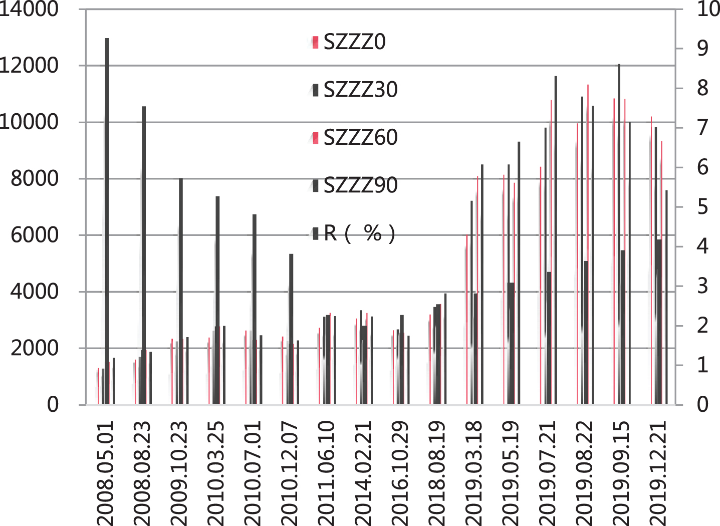
Statistical diagram of interest rates and the Shanghai Composite Index.

The following analyzes the correlation between the interest rate and the Shanghai Composite Index on the 30th day, the Shanghai Composite Index on the 60th day, and the Shanghai Composite Index on the 90th day after the interest rate adjustment. The results are shown in Table 3 and Fig. 2:

OPEN IN VIEWER

Fig. 2

Statistical diagram of the correlation analysis between interest rates and the Shanghai Composite Index.

From Table 2 Amount Fig. 2, we can see that the correlation coefficients of the Shanghai Composite Index on the 30th day after the interest rate adjustment, the Shanghai Composite Index on the 60th day, and the Shanghai Composite Index on the 90th day after the interest rate adjustment are linked. Interest rates and the Shanghai Composite Index on the day of the interest rate adjustment, the Shanghai Composite Index on the 30th day after the interest rate adjustment, the Shanghai Composite Index on the 60th day, and the Shanghai Composite Index on the 90th day showed a negative and weak correlation. Moreover, the correlation between interest rates and the Shanghai Composite Index after interest rate adjustments has increased over time, indicating that the stock market’s response to interest rates is lagging.

Since the correlation relationship is a random mathematical relationship between the sequences, we need to further analyze the cointegration relationship. Through the above analysis, we have obtained the strong correlation between the interest rate and the Shanghai Composite Index on the 90th day after the interest rate adjustment, while the correlation between the Shanghai Composite Index in different periods is also very high. Therefore, we only analyze the relationship between R and SZZZ90. First, we take the logarithm of the variable to get LNR and LNSZZZ90 and perform ADF test. The results are shown in Table 3 and Fig. 3.

OPEN IN VIEWER

Fig. 3

Statistical diagram of ADF test results of LNR and LNSZZZ90.

From the test results in Table 3 and Fig. 3, it can be seen that both LNR and LNSZZZ90 are second-order single integers, that is, I (2) sequences. Since the two are of the same order, the cointegration test can be performed. The test results are shown in Table 4 and Fig. 4.

OPEN IN VIEWER

Fig. 4

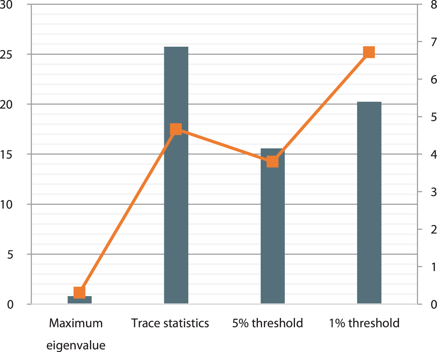
Statistical diagram of Johansen cointegration test results.

The results of the cointegration test show that there is a long-term balanced cointegration relationship between the two variables.

The cointegration test shows that there is a long-term equilibrium cointegration relationship between my country’s one-year time deposit interest rate and the Shanghai Stock Exchange Index. Although the stock market is not very sensitive to interest rates, it is still affected by changes in interest rates, that is, deposit interest rates are lowered, and people transfer part of their original savings to the stock market to obtain returns higher than bank interest. In particular, when the stock market is active, companies will also invest part of their funds into the stock market, and stock prices will rise. However, there is not an absolute one-to-one relationship between interest rates and the Shanghai Composite Index, that is, not every time interest rate drops will cause the stock market to rise, but there will be certain fluctuations. From the correlation coefficient, we also see that there is a negative weak correlation between them. Of course, in the long run, the rapid and sustained development of the stock market is definitely inseparable from the continued low real interest rate. In addition, the impact of interest rate adjustments on the stock market mainly depends on the stock market’s expectations of interest rate adjustments. Only the announcement of information that is not expected by the market can affect the price of the stock market. When the interest rate adjustment has been fully anticipated by the market before the announcement, the announcement of interest rate adjustment information will not have an impact on the market. When the interest rate adjustment information is not expected at all before the announcement, the information announcement will have a relatively large impact on the market. When the market’s information on interest rate adjustment is not complete, the information announcement will have a certain impact on the stock market. However, when the market expects excessive information on interest rate adjustments, once the information is released, stock market prices may even fluctuate in the opposite direction, that is, interest rates fall, and stock prices also fall.

This paper selects (SZZZ) to represent the stock market price fluctuations and selects the economic development level indicator (GDP), money supply indicator (M) and real interest rate indicator (RIR) to represent the factors affecting the stock market. Moreover, this paper still divides the money supply into two levels, M1 and M2. After that, this paper performs logarithmic processing on data other than RIR to obtain LNSZZZ, LNGDP, LNM1 and LNM2. The Johansen cointegration test is performed on LNSZZZ, LNM1, LNGDP and RIR, and the lag order is determined to be 3 according to the AIC information and SC criteria, and the test results are obtained, as shown in Table 5 and Fig. 5.

OPEN IN VIEWER

Fig. 5

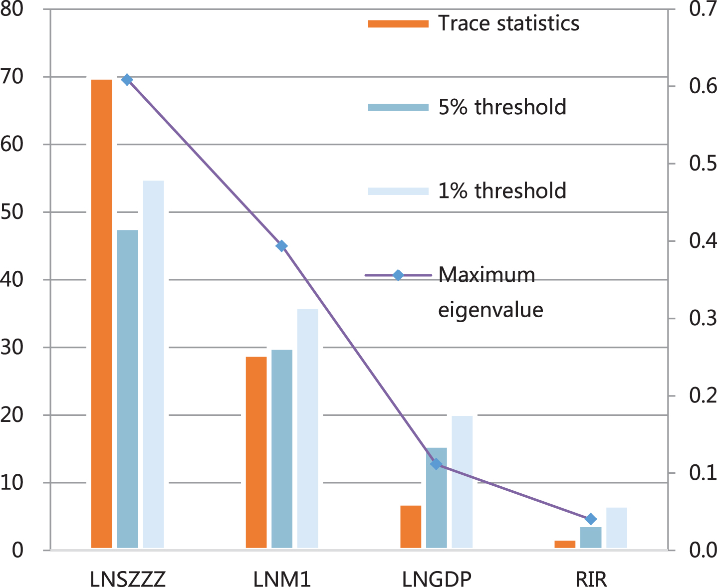
Statistical diagram of Johansen cointegration test results (1).

In this paper, the ADF unit root test is performed on the residual sequence, and it is found that it is already a stationary sequence, which further verifies the correctness of the above cointegration relationship.

The Johansen cointegration test is performed on LNSZZZ, LNM2, LNGDP and RIR, and the lag order is determined to be 3 according to the AIC information and the SC criterion, and the test results are obtained, as shown in Table 6 and Fig. 6.

OPEN IN VIEWER

Fig. 6

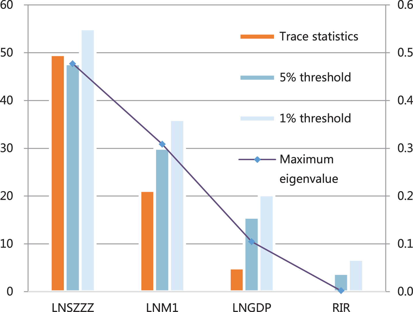
Statistical diagram of Johansen cointegration test results (2).

It can be seen from Table 6 and Fig. 6 that the trace statistic in the first row is greater than the 5% critical value of 47.21, rejecting the null hypothesis that there is no cointegration equation. However, the trace statistic in the second line is less than the 1% critical value 29.68, accepting the null hypothesis of at most one cointegration equation, so there is a long-term balanced cointegration relationship between the variables, and there is only one cointegration equation.

Through the above-mentioned co-integration test, we can conclude that: Both the narrow money supply and the broad money supply have a long-term equilibrium positive correlation with the Shanghai Stock Exchange Index. Moreover, the influence of the narrow money supply on the stock market is greater than the influence of the broad money supply on the stock market.

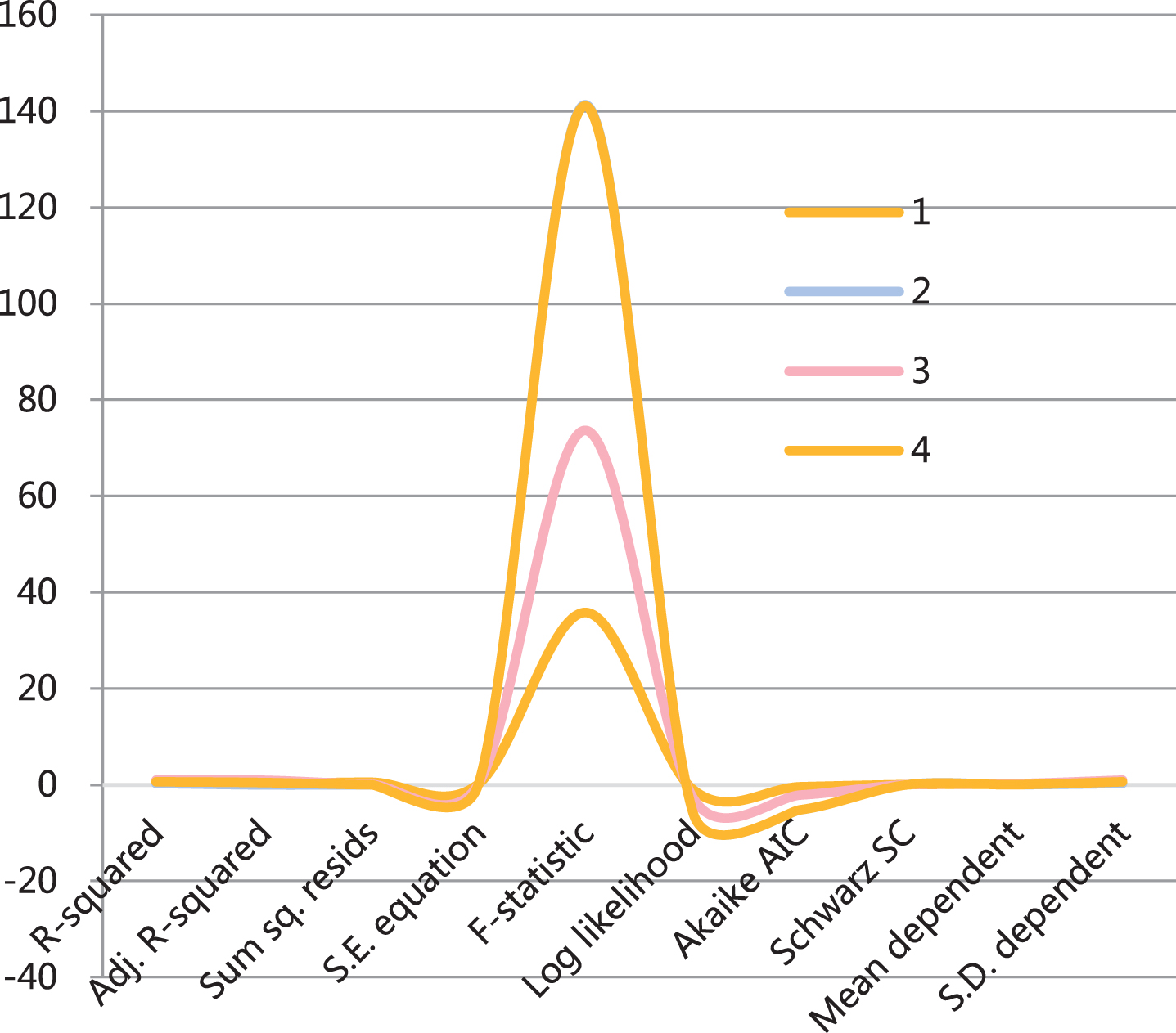
Through the analysis of the above-mentioned co-integration test, there is a co-integration relationship between the Shanghai Stock Exchange Index and related economic variables such as money supply, which meets the conditions for constructing a vector error correction model. Because it is studying the influence of money supply on the development of the stock market, according to the AIC and SC criteria, it is determined that the lag order of VECM is all 3 orders. First, we list the vector error correction model of the impact of variables such as the narrow money supply on the stock market, and the VECM1 test results of the impact of variables such as the narrow money supply on the stock market, as shown in Table 7 and Fig. 7.

OPEN IN VIEWER

Fig. 7

Statistical diagram of VECM1 test results.

It can be seen from the model test results in Table 7 and Fig. 7 that the goodness of fit of the model is better. In addition, it can be seen from the overall test results of the model that the overall effect of the model is still very good.

The VECM1 test results of the influence of variables such as broad money supply on the stock market are shown in Table 8 and Fig. 8.

OPEN IN VIEWER

Fig. 8

Statistical diagram of VECM2 test results.

It can be seen from the model test results in Table 8 and Fig. 8 that although the goodness of fit of the model is average, from the overall test results of the model, the overall effect of the model is very good.

VECM1 shows that there is a significant positive correlation between the short-term dynamic adjustment of LNSZZZ and the narrow money supply of the second and third lagging periods. Although LNSZZZ has a negative correlation with LNM1 which is one lagging period, the coefficient is small. In addition, LNSZZZ has a significant negative correlation with the real interest rates one to three lagging period, and the coefficient is relatively large. VECM2 shows that the short-term LNSZZZ has a negative correlation with the broad money supply in the first and three lag periods, and a positive correlation with the broad money supply in the second lagging period.

In order to further determine the proportion of the error contribution of the above vector error correction models VECM1 and VECM2 from the impact of each component information as the basis for judging the relative importance of each component, we respectively carry out the variance decomposition of the prediction mean square error on LNSZZZ. The results are shown in Table 9 and Table 10. The corresponding statistical graphs are shown in Fig. 9 and Fig. 10.

OPEN IN VIEWER

Fig. 9

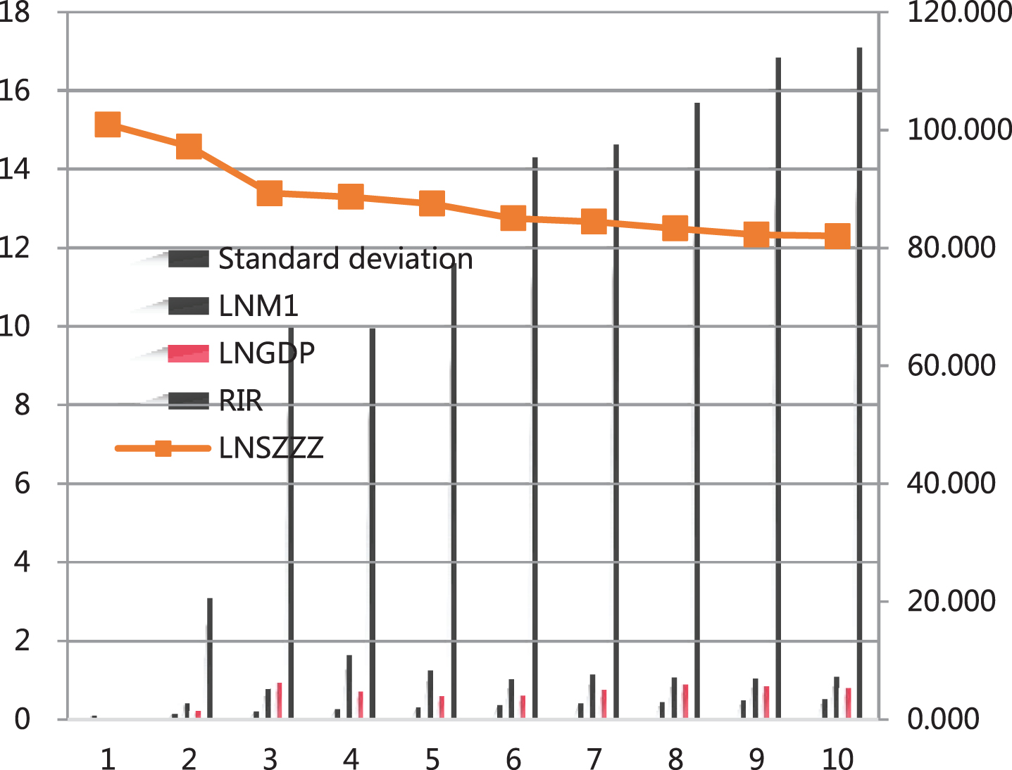
Statistical diagram of variance decomposition 1 of LNSZZZ.

OPEN IN VIEWER

Fig. 10

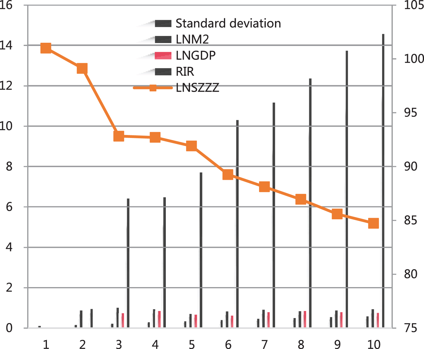
Statistical diagram of variance decomposition 2 of LNSZZZ.

It can be seen from Table 9 and Fig. 9 that the impact of LNSZZZ’s own information has the largest contribution to the prediction error, but it shows a downward trend, with the minimum value reaching 81.21%. The contribution of the narrow money supply to the LNSZZZ forecast variance is small, and it reaches the maximum value of 1.63% in the fourth period. The contribution of the actual interest rate to the LNSZZZ forecast variance is the largest besides its own contribution, and has a clear upward trend, and it reaches the maximum value of 16.91% in the tenth period.

It can be seen from Table 10 and Fig. 10 that LNSZZZ is still the largest contribution of its own information impact to the prediction error, and the minimum is as high as 83.90%. The contribution of broad money supply to LNSZZZ forecast variance is smaller than that of narrow money supply, and the maximum value is only 1.00%.

Through the analysis of co-integration test, this paper finds that there is a long-term stable co-integration relationship between stock market prices and money supply, GDP and interest rates. By constructing a vector error correction model, this paper concludes that the short-term fluctuation of the narrow money supply has a positive impact on the stock market price, while the broad money supply has a negative impact on the stock market in the short term, and the real interest rate has a negative impact on the stock market price in the short term. Through impulse response analysis, we conclude that a random shock to the money supply initially has a negative effect on the stock market. However, as time goes by, it turns into a positive effect and shows a trend of gradual expansion, while the impact of real interest rates has always shown a gradual expansion of negative effects on stock prices. Through the analysis of forecast variance decomposition, it is found that among the forecast errors of forecasting stock market prices, the contribution from the M2 money supply shock is small. However, the contribution from real interest rate shocks is the largest among several variables.