Intelligent English classroom video clarity improvement based on motion compensation and grid flow

Abstract

For the English classroom teaching video denoising algorithm, it is not only necessary to consider whether the noise removal of the output video is thorough, but also to consider the actual operating efficiency and robustness of the algorithm. In the process of the thesis research, after reading a large number of internal and external documents on video denoising algorithms and analyzing the pros and cons of various denoising algorithms, this paper proposes a new video denoising algorithm, which uses the recently proposed grid flow motion model based on camera motion compensation to generate denoised video. Compared with the current advanced video denoising schemes, our method processes noisy frames faster and has good robustness. In addition, this article improves the algorithm framework so that the algorithm can not only deal with offline video denoising, but also deal with online video denoising.

Keywords

Motion compensation grid flow smart classroom English video clarity

1 Introduction

The first use of video in foreign language teaching began in the 1930 s when Disney released movies for non-native English speakers. With the development of cable television, satellite, video technology and the Internet, English video is widely used in teaching all over the world. Nowadays, English videos used in English teaching mainly include BBC, VOA, online English lectures, various English TV programs, English documentaries, English movies, etc., which provide dynamic cultural, language and educational resources, and create multi-modal, multi-media and multi-environmental English listening teaching methods [1].

With the development of network technology and multimedia technology, as well as the application and promotion of online learning platforms, multimedia learning based on words and picture representations to present teaching content together has become more popular. Compared with static documents and commonly used PPT courseware, instructional videos have better compatibility with words and picture representations, so they have become the most important and at the same time the most important multimedia resources in online education and learning. Compared with traditional learning materials, learning materials such as instructional videos have the characteristics of large amount of information and complex temporal and spatial relationships of audiovisual elements. Due to the characteristics of teaching videos, it will increase the cognitive burden of learners to a certain extent and affect their learning effects. In response to these questions in the instructional video, researchers have studied them from different aspects. These studies can be roughly divided into learning clues, subtitle presentation, teaching agency, production costs, and individual differences. The research results also provide positive suggestions for the design and development of instructional videos.

In this context, English video is widely used in English teaching, especially in English listening. The popularity of English video can be proved in English teaching materials design, English listening classroom teaching and English listening test. Judging from the current situation of high school English listening classroom teaching, it can be seen that the listening teaching method is still relatively traditional, that is, the teaching method of “teacher playing audio-student answering-teacher commenting answer” is widely used in listening teaching. This single teaching mode can easily make students bored, dampen their enthusiasm to improve listening ability, and seriously affect the effectiveness of English listening teaching. As more and more English listening skills are combined with other skills in English classes, more and more teachers take the initiative to choose English listening resources suitable for teaching needs and carry out classroom activities for English listening teaching. Moreover, even in the English listening test, the use of multi-modal input is on the agenda. In addition, the listening test based on English video has been piloted in some universities to test the feasibility of its application in large-scale testing [2].

Digital image and its processing technology bring a lot of convenience to the storage, transmission and analysis of video information. However, various analog video signals are still widely used, which brings difficulties to the sharing and analysis of video information. Through the conversion circuit to sample the analog signal, digital images can be obtained, and the digital storage and processing of video information can be realized. For sampled images, spatial resolution is an important indicator of image quality. High resolution means high pixel density and fine details, which not only provides more information, but also facilitates further analysis and processing [3].

2 Related work

The literature [4] proposed the problem of multi-frame super-resolution and gave a frequency domain solution algorithm. The algorithm realizes the use of continuous Fourier and discrete Fourier transform properties without noise and blur and reconstructs a high-resolution image from multiple frames of observation images. Moreover, it expresses the Fourier coefficients of the high-resolution image as a function of a series of registered observation images and solves the function coefficients by calculating a linear equation system. The literature [5] proposed an iterative back-projection algorithm to perform iterative back-projection of the difference between the high-resolution image and the observed image, so as to obtain the estimated value of the high-resolution image. The literature [6] used the median error of different back-projection images to improve the performance of the algorithm based on the existing iterative back-projection algorithm, so that the algorithm has stronger robustness in the presence of abnormal points. Under the assumption that the blur and noise characteristics of all observed images are the same, based on the weighted least squares theory, literature [7] applied the frequency domain method to fuzzy noisy images. The literature [8] proposed a non-iterative spatial data fusion algorithm, which applies this method to pure translation and spatial invariant blur and proposed a fast super resolution algorithm. The literature [9] proposed the POCS algorithm, namely the convex set projection algorithm. The algorithm continuously projects the estimated value of the reconstructed high-resolution image to the conditional convex set. Meanwhile, according to the known data and reasonable assumptions on the signal, each convex set represents a certain constraint on the reconstructed image. The literature [10] proposed a maximum posterior probability algorithm to reconstruct high-resolution images. The literature [11] conducted in-depth research and improvement on its basis. The maximum posterior probability algorithm represents the super-resolution problem as a random estimation problem and makes better use of the prior knowledge of constraints necessary to solve the super-resolution problem. The literature [12] proposed a super-resolution framework to combine the maximum likelihood/maximum posterior probability algorithm with the POCS algorithm, defined a new convex set optimization algorithm, and pointed out the relationship between this algorithm and other existing algorithms. The literature [13] used the generalized Gaussian distribution as the prior distribution of wavelet coefficients and proposed an edge-preserving regularization algorithm in the wavelet domain. The literature [14] proposed a learning-based super-resolution algorithm, applied a training-based algorithm to deal with the super-resolution problem, and used analogy algorithms to calculate between different images. The literature [15] proposed a fast super-resolution algorithm. The algorithm first registers the observed image with the non-uniform high-resolution raster reference frame, uses Delaunay triangulation algorithm to interpolate to obtain a high-resolution image with noise and blur, and then performs deblurring. The literature [16] proposed a new frequency domain algorithm that only uses the low-frequency information of the image for motion estimation. Different from the usual frequency domain algorithms, the performance of this motion estimation algorithm will not be degraded due to noise and strong aliasing, and the estimation performance of rotation and shift parameters is better. The hidden Markov tree model wavelet image interpolation technique proposed in the literature [17] is extended to the field of image super-resolution. The literature [18] used a learning algorithm to achieve super-resolution reconstruction of a single frame image. The super-resolution algorithm based on learning believes that a set of image pixels is a special type of signal set. Compared with a completely random variable sequence, it has fewer changes, and the correspondence between high and low resolution images can be established through neural networks. The literature [19] proposed a new super-resolution algorithm that uses the L1 norm instead of the L2 norm in the usual super-resolution algorithm to find the minimum value, and the edges of the high-resolution images obtained are clearer. The literature [20] proposed the direction CycleSphmiIlg wavelet super-resolution algorithm. The experimental results prove that the algorithm is more adaptable to the edge direction of the image and avoids jagged edges. The literature [21] proposed a new wavelet super-resolution algorithm. According to the transfer characteristics of wavelet coefficients, it uses local correlation coefficients and least squares regression algorithm to achieve detailed subband estimation. According to the wavelet definition, the observed low-resolution image is subjected to unsampled row/column filtering, and the detail subband coefficients are calculated by finding the coefficient neighborhood with the largest correlation value. Since super-resolution reconstruction technology can overcome the inherent resolution limitation of imaging systems, improving the quality of digital images has become a research hotspot in the field of signal processing, and batches of valuable research results have emerged [22].

3 Image video noise classification

Because of the characteristics of noise signals that are different from normal signals, they often have multiple and complex effects on image and video sequences. Noise can be classified according to many dimensions, such as classification according to the source of noise, classification according to the way that noise affects images and video signals, classification according to the spatial probability density distribution characteristics of noise, and so on.

When noise is classified according to the way it affects images and video signals, it can be divided into additive noise and multiplicative noise.

3.1 Additive noise

Additive noise means that the introduced noise interferes with the signal in the form of superposition, and it is statistically independent and uncorrelated with the original image and video signal. For example, the channel noise introduced when image and video signals are transmitted by cables is additive noise. The image or video signal contaminated by additive noise can be expressed by the following formula [23]: $g = f + η$ (1)

Among them, g is an image or video sequence contaminated by noise, f is an ideal image or video signal, and η is the introduced additive noise signal.

3.2 Multiplicative noise

Multiplicative noise means that the introduced noise will change with the change of the original image and video signal, that is, it has correlation with the original image and video signal. It may only be related to the signal of the noisy pixel itself, or it may be related to the signal of the noisy pixel and its neighboring pixels. For example, the grain noise produced by photosensitive film and the noise that obey the Poisson distribution are multiplicative noise. The image or video signal contaminated by multiplicative noise can be expressed by the following formula: $g = f + f \times η$ (2)

Among them, g is an image or video sequence contaminated by noise, f is an ideal image or video signal, and η is the introduced multiplicative noise signal.

As a special signal, noise also belongs to a random process. When classified according to the spatial probability density distribution characteristics of noise, it can be divided into Gaussian noise, Rayleigh noise, gamma noise, exponentially distributed noise, uniformly distributed noise, and impulse noise [24].

3.3 Gaussian noise

Gaussian noise is normally distributed noise, which is also called normal noise. In the space domain and frequency domain, due to the ease of processing of Gaussian noise, Gaussian noise models are often applied in practice. For example, the noise removed in the experimental part of this paper is Gaussian noise. The probability density function of random variables of Gaussian noise can be expressed by the following formula: $p (z) = - \frac{1}{\sqrt{2 π σ}} e^{- {(z - μ)}^{2} / 2 σ^{2}}$ (3)

Among them, z is the pixel gray value, μ is the expectation of z, and σ is the standard deviation of z. When a random variable obeys a Gaussian distribution, 70% of its value falls within the [μ - σ, μ + σ] range, and 95% falls within the [μ - 2σ, μ + 2σ] range. It is usually assumed that the average value μ of z is equal to zero.

3.4 Impulse noise

The probability density function of random variables of impulse noise can be expressed by the following formula: $p (z) = {\begin{matrix} P_{a}, z = a \\ P_{b}, z = b \\ 0 otherwise \end{matrix}$ (4)

If there is b > a, the gray value b will be marked as a bright spot in the image, and the gray value a will be marked as a dark spot. If the value of P_a or P_b is 0, this type of impulse noise is called unipolar impulse noise. If the values of P_a and P_b are not 0, this type of impulse noise is called bipolar impulse noise. In particular, when their values are not 0 and are approximately equal, the impulse noise value will approximate a random distribution on the image, and will be digitized to be similar to the maximum or minimum value of pepper particles and salt particles. Therefore, bipolar impulse noise is also called salt and pepper noise [25].

3.5 Rayleigh noise

The probability density function of the random variable of Rayleigh noise can be expressed by the following formula: $p (z) = {\begin{matrix} \frac{2}{b} (z - a) e^{[- {(z - a)}^{2} / b]} & z ⩾ a \\ 0 & z < a \end{matrix}$ (5)

The mean and variance are as follows: ${\begin{matrix} μ = a + \sqrt{π b / 4} \\ σ^{2} = b (4 - π) / 4 \end{matrix}$ (6)

The probability density function of the random variable of the gamma noise can be expressed by the following formula: $p (z) = {\begin{matrix} \frac{a^{b_{z}} z^{b - 1}}{(b - 1)} e^{- x} & z ⩾ 0 \\ 0 & z < 0 \end{matrix}$ (7)

Among them, there is a > 0. b is a positive integer and “!” means factorial. The mean and variance are as follows: ${\begin{matrix} μ = \frac{b}{a} \\ σ^{2} = \frac{b}{a^{2}} \end{matrix}$ (8)

3.6 Exponentially distributed noise

The probability density function of the random variable of the exponentially distributed noise can be expressed by the following formula: $p (z) = {\begin{matrix} {az}^{- ax} & z ⩾ 0 \\ 0 & z < 0 \end{matrix}$ (9)

Among them, there is a > 0, and mean and variance are as follows ${\begin{matrix} μ = \frac{1}{a} \\ σ^{2} = \frac{1}{a^{2}} \end{matrix}$ (10)

3.7 Uniform noise

The probability density function of random variables of uniform noise is as follows: $p (z) = {\begin{matrix} \frac{1}{b - a} & a ⩽ z ⩽ b \\ 0 & otherwise \end{matrix}$ (11)

Its mean and variance are represented by the following formula: ${\begin{matrix} μ = \frac{a + b}{2} \\ σ^{2} = \frac{{(b - a)}^{2}}{12} \end{matrix}$ (12)

The probability density function of the random variable of Poisson noise is as follows: $p (z) = \frac{{(λ f)}^{z}}{z!} e^{- λ f}$ (13)

Among them, z is the pixel gray value and obeys the Poisson distribution, f is the light intensity, and λ is the noise factor.

The image and video sequence after denoising processing needs a series of evaluation criteria and methods to determine the denoising effect. Initially, people make subjective evaluation based on the intuitive feeling brought by vision. However, this method is too subjective and difficult to be unified and standardized. With a lot of research and experimental comparison, researchers have proposed a series of rigorous and objective evaluation criteria, which use digital indicators to evaluate the performance of denoising [26].

Subjective evaluation is the subjective evaluation of the visual effect of the image by the recipient through observing the image and obtain the result. Subjective evaluation has a lot to do with the characteristics of the observer itself, as well as factors such as observation conditions. Observers can conduct comprehensive evaluation by comparing the denoised image with the original noisy image, or comparing the denoised image with different denoising methods. In fact, because noise pollution will inevitably cause information loss and cannot be reproduced by denoising, no matter how excellent denoising algorithms are, it is impossible to completely restore images or video sequences contaminated by noise to a noise-free level. Therefore, the consistency of the denoised image and the original image can only be used as a reference. The criteria for subjective evaluation vary from person to person. It can mainly evaluate the denoising effect from two aspects: observing the effect of noise smoothing and the change of image detail information before and after denoising. Whether the image details can be protected to the greatest extent while denoising is the core of judging the performance of denoising, and it is also the difficulty that denoising technology is trying to overcome and improve.

3.8 Objective criteria

For any image, methods such as PSNR (Peak Signal to Noise Ratio) and SSIM (Structural Similarity index) can be used to evaluate the image quality.

A noise-free clean image g (i, j) of size M × N and a noisy image are given as follows: $MSE = \frac{1}{MN} \sum_{i = 0}^{M - 1} \sum_{j = 0}^{N - 1} E {{[g (i, j) - f (i, j)]}^{2}}$ (14)

Then, the peak signal-to-noise ratio PSNR (unit: dB) of the image can be expressed by the following formula: $PSNR = 10 log \frac{A^{2}}{MSE}$ (15)

Among them, A represents the maximum gray value of the pixel, for example, the maximum gray value of an 8-bit image is 255. Usually, if the pixel value is represented by B-bit binary, then there is A = 2^B - 1. The image quality is directly proportional to the image PSNR value. The larger the image PSNR, the better the denoising effect.

Structural similarity SSIM is an index used to measure the similarity of two images. Two images x and y are given, the structural similarity SSIM of the two images can be expressed by the following formula: $SSIM (x, y) = \frac{(2 μ_{x} μ_{y} + c_{1}) (2 σ_{xy} + c_{2})}{(μ_{x}^{2} μ_{y}^{2} + c_{1}) (σ_{x}^{2} + σ_{y}^{2} + c_{2})}$ (16)

Among them, μ_x is the average value of x, μ_y is the average value of y, and $σ_{x}^{2}$ is the variance of x. At the same time, $σ_{y}^{2}$ is the variance of y, and σ_xy is the covariance of x and y. c₁ = (K₁L) ² and c₂ = (K₂L) ² are constants used to maintain stability. L is the dynamic range of pixel values.

The range of SSIM is 0 to 1. When the two images are the same, the value of SSIM is equal to 1. The larger the SSIM value of the image, the better the denoising effect.

When different denoising methods are used to denoise, the peak signal-to-noise ratio and structural similarity of the original image and the denoised image are calculated. By comparing the PSNR and SSIM values of different denoising methods, the performance pros and cons of different denoising methods can be obtained from objective data. The comparison of denoising performance of algorithms in Chapter 4 of this paper will use PSNR SSIM indicators.

4 KLT tracking algorithm

The Kanade-Lucas-Tomasi tracking algorithm is a corner tracking algorithm, which is also called the LK optical flow tracking method. Gibson first proposed the concept of optical flow. Optical flow is a characterization of the instantaneous velocity of the pixel motion of the space moving object on the observation imaging plane. It uses the changes in the time domain of pixels in the image sequence and the correlation between adjacent frames to determine the correspondence between the previous frame and the current frame, thereby calculating the object motion information between adjacent frames method. Optical flow is distinguished according to sparse optical flow and dense optical flow. Both belong to image registration methods. However, unlike dense optical flow, which needs to calculate the offset of all points on the image, sparse optical flow is only calculated for several interesting feature points on the image, thus forming a sparse optical flow field. Since there is no need to accurately calculate the offset of each point, the amount of calculation is much lower than that of dense optical flow. However, the accuracy of image registration through this sparse optical flow field is lower than that of dense optical flow. A batch of discrete feature points are detected through FAST features, and then these feature points are tracked through KLT to obtain the matching relationship between adjacent frames.

The basic assumptions of optical flow have the following three points:

The influence of the external environment on adjacent frames is not considered, that is, the brightness between adjacent video frames is consistent;

The time between adjacent video frames is continuous, or the movement of objects between adjacent frames does not appear to be transient;

Spatial consistency. That is, the neighboring stores in a scene projected on the image are also neighboring stores, and the speed of the neighboring points is the same.

Now, we assume that a certain pixel is located at (x, y, t) on the image, its pixel brightness is I (x, y, t), and the distance that the pixel moves between two frames is ΔxΔyΔt. From the Taylor expansion, the following formula can be obtained: $\begin{matrix} I (x + Δ x, y + Δ y, t + Δ t) = I (x, y, t) + \\ \frac{\partial I}{\partial x} Δ x + \frac{\partial I}{\partial y} Δ y + \frac{\partial I}{\partial z} Δ z + o \end{matrix}$ (17)

From the assumption, we know $I (x + Δ x, y + Δ y, t + Δ t) = I (x, y, t)$ (18)

Therefore, the following formula is obtained: $\frac{\partial I}{\partial x} \frac{Δ x}{Δ t} + \frac{\partial I}{\partial y} \frac{Δ y}{Δ t} + \frac{\partial I}{\partial t} = 0$ (19)

Among them, $\frac{Δ x}{Δ t}$ and $\frac{Δ y}{Δ t}$ are the optical flow of the point in the x and y directions, and $\frac{\partial I}{\partial t}$ represents the change in time of the pixel.

The KLT method was originally used to meet the needs of the LK optical flow method to select suitable feature points. It first creates a time window of a certain size in two adjacent frames, then finds the displacement that minimizes the sum of the squares of the pixel intensity difference between the two windows, and then approximates the movement direction of all pixels in the window to the displacement vector. However, the pixels do not move regularly, and the moving directions of the pixels in the window are not consistent. Therefore, such an approximation will inevitably lead to errors. How to select the appropriate window or feature point to obtain the most accurate tracking is the key to the problem. The KLT algorithm is to select a feature point suitable for tracking. It believes that the definition of a good feature point should be able to be well tracked. The KLT algorithm makes full use of spatial characteristics, and it can find the feature matching information between images faster than traditional corner tracking methods.

5 Robustness of grid flow motion model

High-quality feature points are often evenly distributed in each area of the image, and will not be affected by factors such as illumination. The number of feature point pairs in some adjacent frames may be relatively small. If each frame of the video can cover rich and dense feature points, each vertex can receive more motion vectors. When selecting good feature points for tracking, there are often fewer feature points in areas with fuzzy textures (such as the ground and sky) because the threshold is biased by other highly textured areas and a large number of feature points are filtered out. Therefore, the image is divided into blocks and features are extracted independently for each sub-region. Moreover, the threshold of FAST detection feature is not fixed, but it will be dynamically adjusted according to the divided area. In this way, the feature points can be maximized without regional differentiation, but can be evenly distributed in the entire image as much as possible to ensure that there are a certain number of feature points in each area of the image.

5.1 Outlier filtering

In 1981, the random consensus algorithm (RANSAC) proposed by Fischler and Bolles et al. is an algorithm that calculates the mathematical model parameters of the data based on a set of sample data sets containing abnormal data to obtain valid sample data. The RANSAC algorithm is often used in computer vision and image processing. The basic assumption is that a data set contains correct data (Inliers) and abnormal data (Outliers), that is, the data set contains noise. Among them, the correct data refers to the data that can be adapted to the mathematical model within the normal range. Abnormal data refers to data that exceeds the normal range and cannot be applied by mathematical models. At the same time, RANSAC also assumes that when a set of correct data is given, the RANSAC algorithm can eliminate abnormal data sets through random sampling, find the model that satisfies the most sample points, and screen out the correct data sample set.

The RANSAC algorithm is often used to remove the outliers in the feature points to improve the robustness of the motion path estimation. However, because the grid stream wants to retain the motion vectors that do not exist in the global linear space, this method is not suitable for this application scenario. By dividing the image into sub-images of 4 × 4, and filtering out the outliers through the local homomorphic fitting of RANSAC, the wrongly matched feature points and large deviation motion vectors can be successfully filtered out.

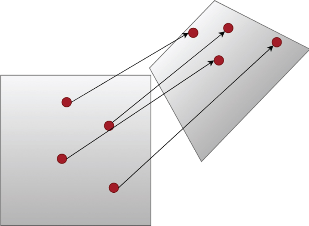
Projection transformation is shown in Fig. 1. It is also called homography transformation, which is a mapping relationship from one plane to another. The goal of projective transformation is to get the homography matrix through given pairs of points. Its mathematical expression can be represented by the following formula: $[\begin{matrix} x^{'} \\ y^{'} \\ 1 \end{matrix}] = [\begin{matrix} a & b & t_{x} \\ c & d & t_{y} \\ v_{x} & v_{y} & 1 \end{matrix}] [\begin{matrix} x \\ y \\ 1 \end{matrix}]$ (20)

Fig.1

Projection transformation.

Projection transformation is a non-singular linear transformation under homogeneous coordinates. The parallel image edges before transformation may be inclined after transformation, but the original collinear points are not affected before and after the transformation.

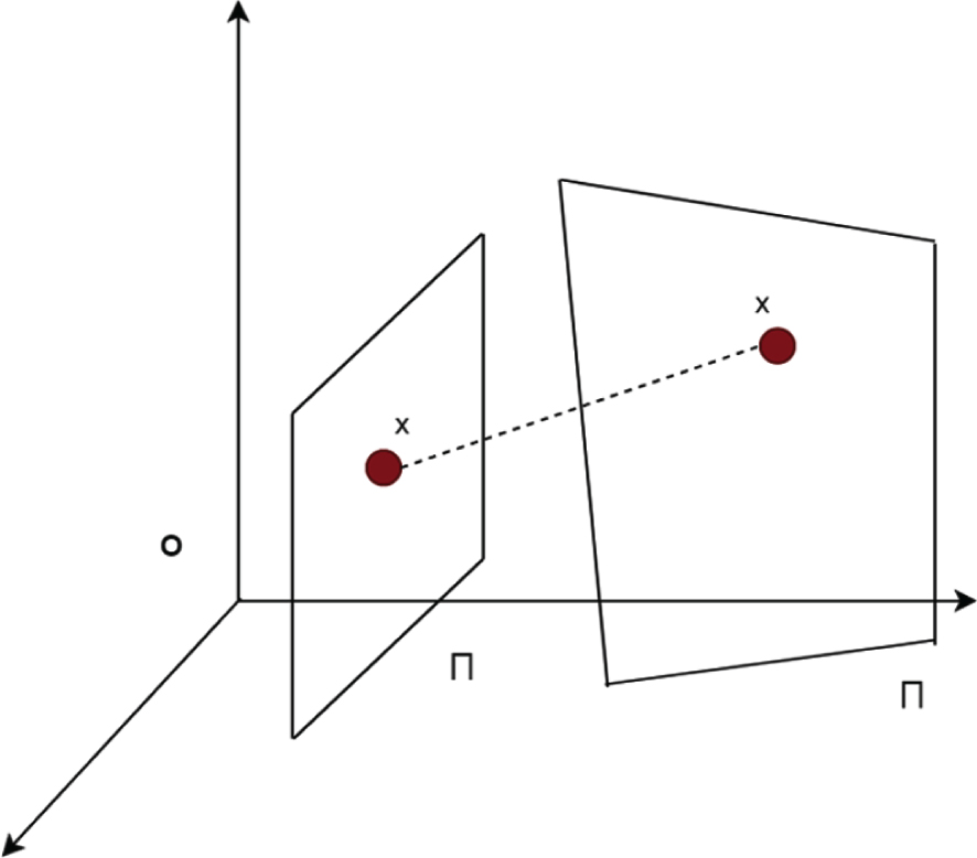
The projection transformation model has practical geometric significance. As shown in Fig. 2, all points x on plane A can be mapped from all points x′ on plane B with O as the center. When two planes have such a mapping relationship, A is called the projection transformation plane of B. We assume that $(p, \hat{p})$ is the p-th matched feature pair. Among them, p is in the t-th frame, $\hat{p}$ is in the t–1-th frame, and $p, \hat{p}$ is the coordinate of the feature point of the image. Then, the motion vector at the feature point p of the t-th frame is: ${\vec{v}}_{p} = p - \hat{p}$ (21)

Fig.2

The geometric meaning of the projection transformation model.

Before estimating the grid flow, $\hat{p}$ is subjected to a homography transformation F_t to obtain a motion vector V_t from the t–1-th frame to the t-th frame. At this time, the local residual motion vector at the feature point $\hat{p}$ is: $v_{p}^{'} = p - F_{t} \hat{p}$ (22)

The final grid flow vector is: $v_{p} = V_{t} + v_{p}^{'}$ (23)

The mesh flow motion model (Mesh Flow Motion Model) is a spatially smooth sparse motion field. It is a non-parametric motion model, which consists of sparse motion vectors located at the vertices of the mesh, and can be used to estimate the motion between adjacent frames. In this section, the mesh flow motion model will be introduced in detail. Figure 3 shows the comparison between Steady Flow and grid flow. The steady flow calculates the dense optical flow and extracts the pixel contours of all pixel positions for motion estimation, while the grid flow is computationally cheaper.

Fig.3

Comparison of pixel contours of steady flow and grid flow.

Each matching feature point pair of the original English classroom image produces one as shown in Fig. 4(a). In the implemented estimation, the grid stream calculates the motion vector between the current frame and the previous frame. The current frame is divided into regular grids, and the motion vectors matched by the feature points are propagated to the grid vertices within the designated circle nearby, as shown in Fig. 4(b). When the propagation is completed, each vertex may receive multiple motion vectors from different feature points.

Fig.4

Motion vector propagation.

Figure 5 is an improved flow chart of frame deformation. In figure (a), including the current frame, the frames before and after the current frame, all frames are aligned with the common key frame. In the fusion window in Figure (b), since all frames are aligned, pixel fusion can be performed. The fusion process does not change. Then, the denoised frame is deformed back to the original position, and the deformed copy of the current frame will remain in the window to continue denoising the subsequent frames. In this way, during the denoising process of each frame, only two frame deformation processing are involved. If one deformation takes 5 milliseconds, the two deformations consume 10 milliseconds, and the processing speed is about 100FPS. The processing speed of the frame is much better than the original frame without optimized deformation process.

Fig.5

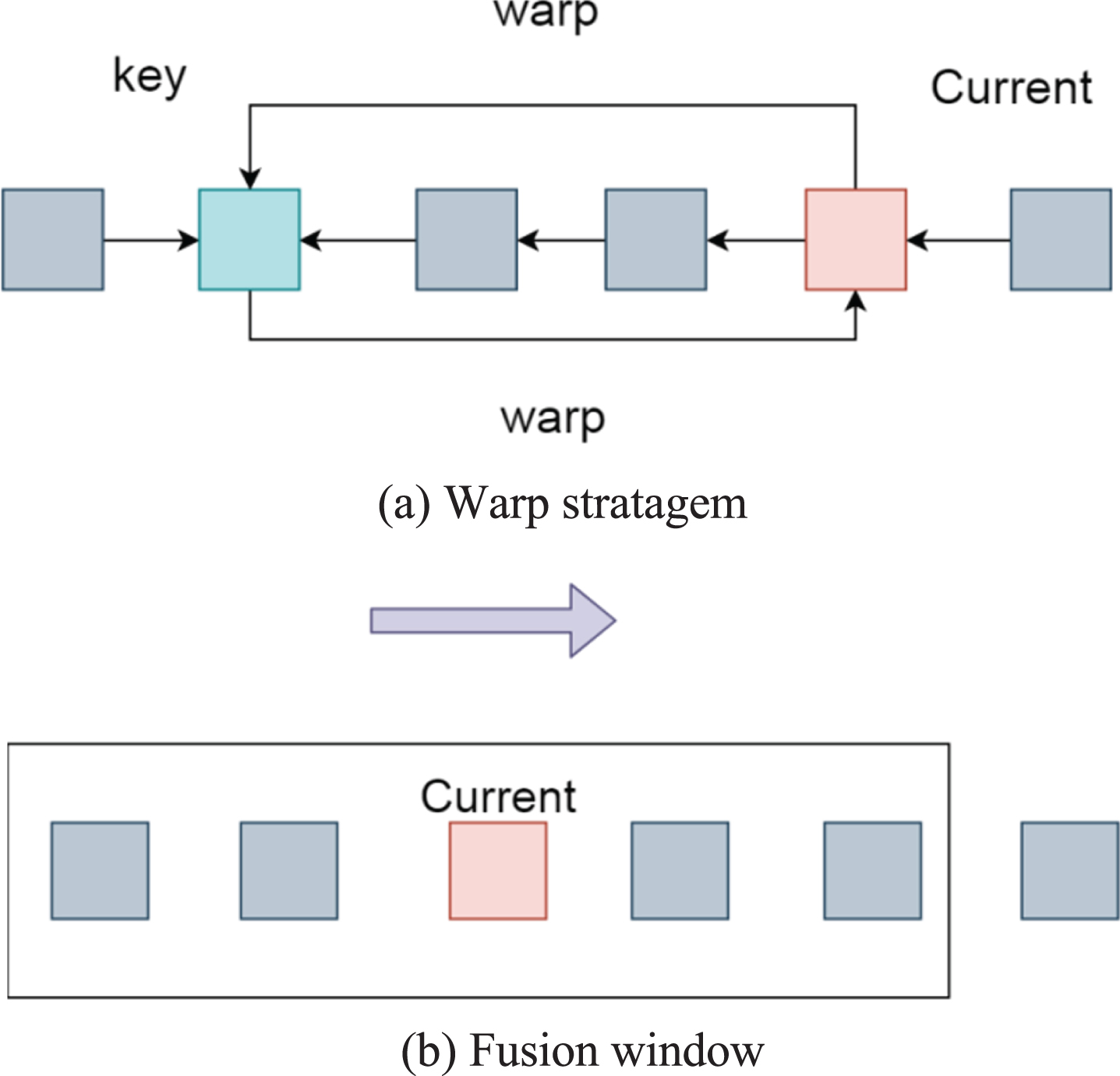
Improved frame deformation flowchart.

There are composite video systems that use interlaced scanning technology to display images on the screen. Figure 6 below shows the concept of interlaced scanning. The analog video signal includes a control scan, which scans from left to right line by line and from top to bottom field by field. Two interleaved fields are combined into a complete frame, the first field is an odd field, and the second field is an even field.

Fig.6

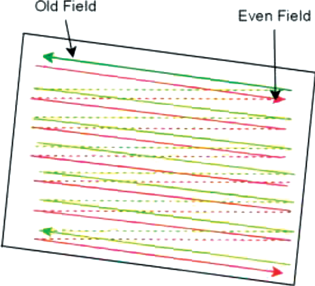
Schematic diagram of interlaced scanning.

6 Model performance analysis

For further comparison, this article first selects the FPGA hardware acceleration schemes and related filtering algorithms of other denoising algorithms proposed before for objective performance comparison, as shown in Tables 1 and 2. The corresponding statistical graphs are shown in Figs. 7–10. On the one hand, the denoising algorithm in this paper is better than other algorithms in denoising performance. On the other hand, due to the low complexity of the algorithm itself and the realization of only part of the modules in the algorithm, the FPGA in this solution only consumes fewer logic units.

Table 1
Performance comparison between the algorithm in this paper and other filtering algorithm

2 5 10 15 Average

Original noise image PSNR 42.43 34.50 28.43 24.95 32.58

SSIM 0.99 0.91 0.76 0.65 0.83

Total variation filtering PSNR 42.64 33.93 28.82 26.38 32.95

SSIM 1.00 0.96 0.89 0.83 0.92

Extended trilateral filter PSNR 43.19 35.49 30.56 28.09 34.33

SSIM 1.00 0.97 0.90 0.83 0.92

Paper model PNSR 43.73 36.57 31.36 28.64 35.08

SSIM 1.00 0.98 0.94 0.88 0.95

		2	5	10	15	Average
Original noise image	PSNR	42.43	34.50	28.43	24.95	32.58
SSIM	0.99	0.91	0.76	0.65	0.83
Total variation filtering	PSNR	42.64	33.93	28.82	26.38	32.95
SSIM	1.00	0.96	0.89	0.83	0.92
Extended trilateral filter	PSNR	43.19	35.49	30.56	28.09	34.33
SSIM	1.00	0.97	0.90	0.83	0.92
Paper model	PNSR	43.73	36.57	31.36	28.64	35.08
SSIM	1.00	0.98	0.94	0.88	0.95

Table 2

The performance comparison between the improved BM3D algorithm in this paper and the three-dimensional mean algorithm

		2	5	10	15	Average
Original noise image	PSNR	42.43	34.50	28.43	24.95	32.58
SSIM	0.99	0.91	0.76	0.65	0.83
Improved BM3D algorithm	PSNR	43.58	36.33	31.13	28.48	34.89
SSIM	1.00	0.98	0.93	0.88	0.95
Algorithm of this paper	PSNR	43.73	36.57	31.36	28.64	35.08
SSIM	1.00	0.98	0.94	0.88	0.95

Fig.7

PSNR statistics 1 of algorithms.

Fig.8

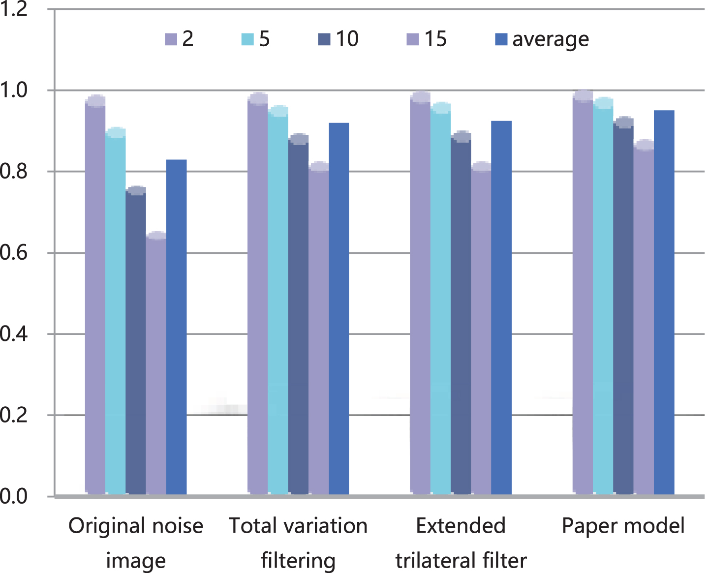
SSIM statistics 1 of algorithms.

Fig.9

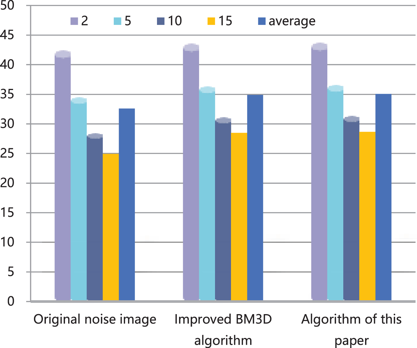
PSNR statistics 2 of algorithms.

Fig.10

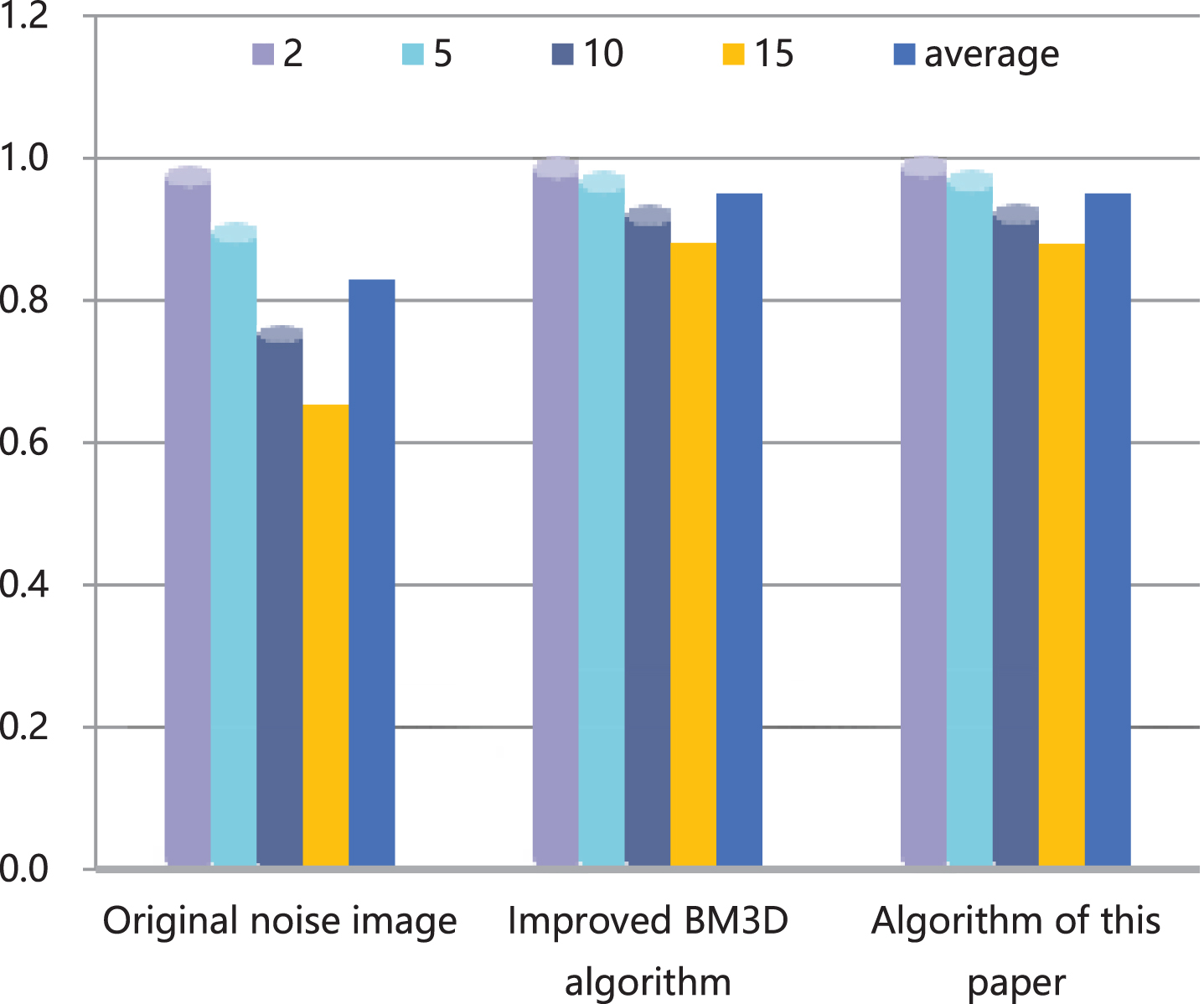
SSIM statistics 2 of algorithms.

In addition, through the analysis of the data in the table, it can be seen that the architecture proposed in this paper has excellent performance in terms of throughput and resource occupancy costs.

It can be seen from the above chart that the model constructed in this article can play a good role in improving the clarity of intelligent English classroom videos, and the model constructed in this article can achieve the expected effect.

7 Conclusion

With the continuous development of digital multimedia technology in English classrooms, the requirements for the quality of the obtained video images are constantly increasing, and the pursuit of high-definition and high-quality videos and pictures is more and more. In the actual collection and transmission of video images, the noise introduced will seriously affect the viewer’s visual experience. Therefore, the video image denoising technology came into being, that is, as accurately as possible to recover the original image that retains the important image details from the observed noise image. On the other hand, video image denoising technology, as a crucial step in image and video preprocessing, determines the accuracy of many post-processing algorithms including visual enhancement, feature extraction, target recognition and target segmentation. Therefore, this paper proposes a new video denoising algorithm, which uses the recently proposed grid flow motion model based on camera motion compensation to generate clearer video after noise removal. Compared with the current advanced video denoising schemes, our method processes noisy frames faster and has good robustness. In addition, this article improves the algorithm framework so that the algorithm can not only deal with offline video denoising, but also deal with online video denoising.

Footnotes

Acknowledgment

This paper was Funed by the Research and Innovation Team of Wuhan Technical College of Communications (Project NO: CX2018A13).

References

Wang

, Shi

, Shu

, et al. Embedded manifold-based kernel fisher discriminant analysis for face recognition, Neural Processing Letters 43(1) (2016), 1–16.

Chuk

, Chan

A.B.

and Hsiao

J.H.

, Understanding eye movements in face recognition using hidden Markov models, Journal of Vision 14(11) (2014), 8–8.

Hamdi Bouchech, Selection of optimal narrowband multispectral images for face recognition, Monthly Notices of the Royal Astronomical Society 402(4) (2015), 2140–2186.

Ramachandra

and Busch

, Presentation attack detection methods for face recognition systems: A comprehensive survey ACM Computing Surveys 50(1) (2017), 8.1–8.37.

Huang

, Shan

, Wang

, et al. A benchmark and comparative study of video-based face recognition on COX face database, IEEE Transactions on Image Processing 24(12) (2015), 5967–5981.

Wei

C.P.

and Wang

Y.C.F.

, Undersampled face recognition via robust auxiliary dictionary learning, Image Processing IEEE Transactions on 24(6) (2015), 1722–1734.

Ajit Krisshna

N.L.

, Deepak

V.K.

, Manikantan

, et al. Face recognition using transform domain feature extraction and PSO-based feature selection, Applied Soft Computing 22(6) (2014), 141–161.

Weng

, Lu

and Tan

Y.P.

, Robust point set matching for partial face recognition, Image Processing IEEE Transactions on 25(3) (2016), 1163–1176.

Cui

, Chang

, Shan

, et al. Joint sparse representation for video-based face recognition, Neurocomputing 135(5) (2014), 306–312.

10.

Phillips

P.J.

and Otoole

A.J.

, Comparison of human and computer performance across face recognition experiments, Image and Vision Computing 32(1) (2014), 74–85.

11.

Tang

, Zhu

, Yu

, et al. A novel sparse representation method based on virtual samples for face recognition, Neural Computing & Applications 24(3–4) (2014), 513–519.

12.

Mehta

, Yuan

and Egiazarian

, Face recognition using scale-adaptive directional and textural features, Pattern Recognition 47(5) (2014), 1846–1858.

13.

Raghavendra

, Raja

K.B.

and Busch

, Presentation attack detection for face recognition using light field camera, IEEE Transactions on Image Processing 24(3) (2015), 1060–1075.

14.

Yang

, Zhu

, Liu

, et al. Joint representation and pattern learning for robust face recognition, Neurocomputing 168(30) (2015), 70–80.

15.

Yan

, Wang

and Suter

, Multi-subregion based correlation filter bank for robust face recognition, Pattern Recognition 47(11) (2014), 3487–3501.

16.

Fan

, Ni

, Zhu

, et al. Weighted sparse representation for face recognition, Neurocomputing 151(3) (2015), 304–309.

17.

Tang

, Feng

and Cai

, Weighted group sparse representation for undersampled face recognition, Neurocomputing 145(5) (2014), 402–415.

18.

Al-Arashi

W.H.

, Ibrahim

and Suandi

S.A.

, Optimizing principal component analysis performance for face recognition using genetic algorithm, Neurocomputing 128(27) (2014), 415–420.

19.

Morelli Andrés

, Padovani

, Tepper

, et al. Face recognition on partially occluded images using compressed sensing, Pattern Recognition Letters 36(1) (2014), 235–242.

20.

Ding

and Tao

, Pose-invariant face recognition with homography-based normalization, Pattern Recognition 66 (2017), 144–152.

21.

Yang

, Feng

, Shiu

S.C.K.

, et al. Fast and robust face recognition via coding residual map learning based adaptive masking, Pattern Recognition 47(2) (2014), 535–543.

22.

Zhu

and Li

, A kernel-based sparse representation method for face recognition, Neural Computing & Applications 24(3–4) (2014), 845–852.

23.

Chen

W.S.

, Zhao

, Pan

, et al. Supervised kernel nonnegative matrix factorization for face recognition, Neurocomputing 205(12) (2016), 165–181.

24.

, Gong

, Li

, et al. Learning compact feature descriptor and adaptive matching framework for face recognition, image processing, IEEE Transactions on 24(9) (2015), 2736–2745.

25.

Zhao

, Zhou

and Cao

, Human face recognition based on ensemble of polyharmonic extreme learning machine, Neural Computing & Applications 24(6) (2014), 1317–1326.

26.

Gaidhane,

Vilas H

, Hote,

Yogesh V

, Singh,

Vijander

, An efficient approach for face recognition based on common eigenvalues, Pattern Recognition 47(5) (2014), 1869–1879.