Iterative learning control of an inverse novel ball screw transmission system

Abstract

Iterative Learning Control is a branch of intelligent control which combines artificial intelligence and control theory. This objective of this study aims at reducing the cyclic error of an inverse ball screw transmission system by using iterative learning control approach. Firstly, kinematic and dynamic analyses are conducted by using the vectorial loop closure and Lagrange equations, respectively. Then, system identification is performed followed by controller design. Moreover, controller parameters are optimized to minimize the error. Finally, the feasibility and the effectiveness of the proposed approach are verified by computer simulation and prototype experiment. The experimental results showed that the reducing percentage of the square error sum of the output speed is 90.64% by using PID control only. If ILC is applied additionally, the error is further reduced to 94.21%. Therefore, the proposed approach is not only feasible and but also effective.

Keywords

Ball screw ILC controller PID controller Oldham coupling

1 Introduction

With the advantages of its low friction, high precision, and longer service, ball screws are widely used in various kind of precision or automatic machinery. Ball screws are mechanisms which converting motion between rotation and rectilinear motion by direct contact. It mainly consists of a screw, a cap, and balls circulating between the former two, as shown in Fig. 1 [1].

Fig. 1

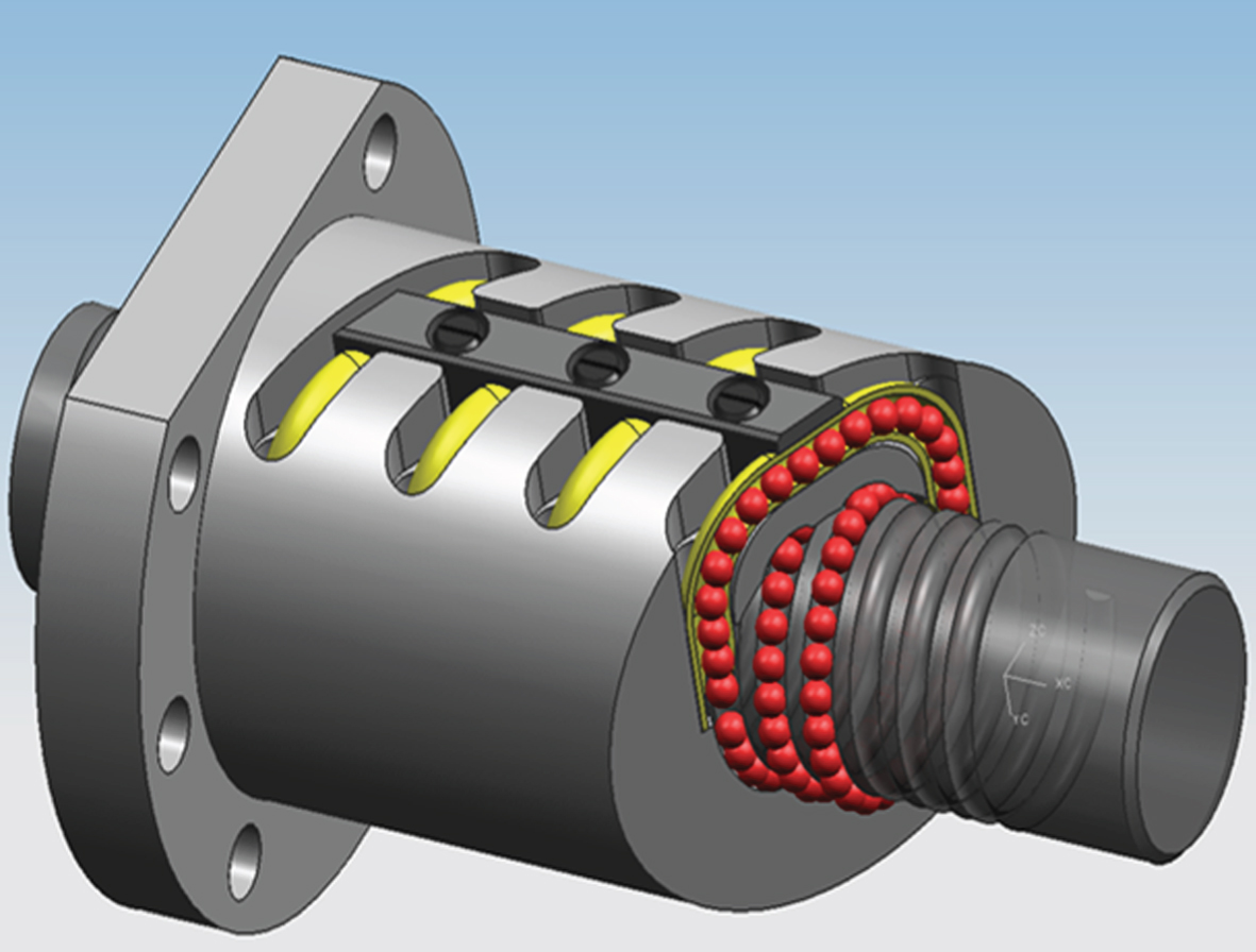
Ball screw [1].

Typical applications of ball screws are power steering [2], machine tool feed drives [3, 4], precision positioning stage [5], etc., which convert rotatory motion into rectilinear motion. However, an ever increasing demand is to convert rectilinear motion into rotatory motion, e.g., energy harvesters [6, 7] and regenerative shock absorbers [8, 9]. These ball screws are called inverse ball screws in this study, i.e., the cap is the driver that produces rectilinear motion, and then drives the screw to generate rotatory motion. Nevertheless, precision control studies on this topic are hardly found. In 2014, Hsieh & Chang [1] established the system model of an inverse ball screw system, and performed a refined control to enhance its output accuracy.

Iterative Learning Control (ILC) has been well developed in the past. In 1978, Uchiyama [10] firstly proposed the concept of iterative learning to improve the motion trajectory of robots at high speed. In 1984, Arimoto et al. [11] proposed a simple PID-type learning algorithm, which ensured the convergence of the learning system under certain conditions. In 2008, Madady [12] proposed an optimum design approach for determining the PID coefficients which ensure the convergence of the learning system. ILC has been applied in various applications, e.g., motor control [13 –15], robots [16 –18], machine tools [19, 20].

This objective of this study aims at reducing the cyclic error of an inverse ball screw transmission system by using iterative learning control approach, hence it can produce output motions with high accuracy. In the following sections, Sec. 2 introduces the composition of the system along with its kinematic and dynamic analyses. Sec. 3 presents the approach of hybrid control. An illustrative design example is given in Sec. 4. Sec. 5 conducts prototype experiments. Finally, major conclusions are summarized in Sec. 6.

2 Inverse ball screw system

The inverse ball screw system proposed in [1] consists of a motor with a gear reducer (not shown), a variable speed coupling, a slider-crank mechanism, and a ball screw, as shown in Fig. 2. The slider-crank mechanism is driven by the motor through a generalized Oldham coupling, and then it drive the ball screw to produce a non-uniform rotational output.

Fig. 2

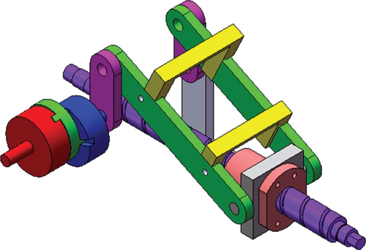
Inverse ball screw system [1].

A generalized coupling can be, kinematically equivalent, converted into a four-bar linkage [21 –23]. To modelling the system dynamic, kinematic and dynamic analyses have to be conducted firstly. The vector closure approach is used for the analyses in this study. Therefore, the proposed system is firstly transformed into its equivalent linkage, as shown in Fig. 3. Its associated vectorial representation is shown in Fig. 4 where ϕ is the angular position of the screw For simplification, the line connected fixed pivots a₀b₀ is then assumed to be parallel with t the slider’s motion. Finally, it can be found that it is a planar linkage with 6 links and 7 joints, the ball screw is not considered in the analysis.

Fig. 3

Equivalent mechanism [24].

Fig. 4

Vectorial representation [24].

2.1 Kinematic analysis

The details of the kinematic analysis can be found in [24], and will be repeated here. The angular position is $ϕ = \frac{2 π}{p} (r_{1} + r_{4} cos θ_{4} + r_{5} cos θ_{5})$ (1) the angular velocity and the angular acceleration, respectively, are $\dot{ϕ} = - \frac{2 π}{p} (r_{4} sin θ_{4} {\dot{θ}}_{4} + r_{5} sin θ_{5} {\dot{θ}}_{5})$ (2) and

$\begin{matrix} \ddot{ϕ} = & \frac{2 π}{p} (r_{4} sin θ_{4} {\ddot{θ}}_{4} - r_{4} cos θ_{4} {\dot{θ}}_{4}^{2} \\ + r_{5} sin θ_{5} {\ddot{θ}}_{5} + r_{5} cos θ_{5} {\dot{θ}}_{5}^{2}) \end{matrix}$ (3)

2.2 Dynamic analysis

To establish a system model, it is required to perform dynamic analysis to obtain its equation of motion. In this study, the Lagrange equation approach is used for the analysis. Figure 5 shows the dimensions of the mechanism. Let G_i = (x_i, y_i), i = 1–3, be the mass center of the link i, it yields

Fig. 5

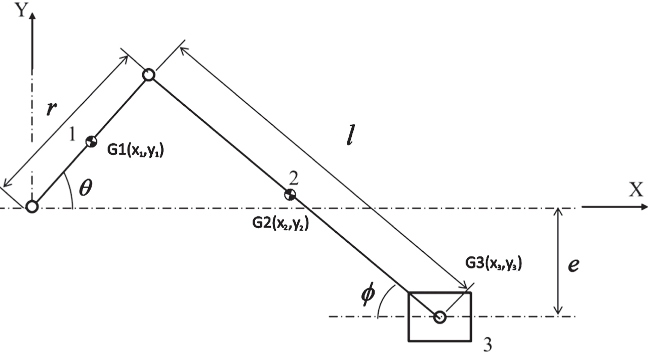
Dimensions.

$G_{1} (x_{1}, y_{1}) = (\frac{r cos θ}{2}, \frac{r sin θ}{2})$ (4) $G_{2} (x_{2}, y_{2}) = (r cos θ + \frac{l cos θ}{2}, r sin θ - \frac{1}{2} l sin ϕ)$ (5) $G_{3} (x_{3}, y_{3}) = (r cos θ + l cos ϕ, r sin θ + l sin ϕ)$ (6)

The kinematic energy T_i (i = 1-3) of each link can be expressed as $T_{1} = \frac{1}{2} I_{1} \dot{θ} = \frac{1}{6} m_{1} r^{2} {\dot{θ}}^{2}$ (7) $T_{2} = \frac{1}{6} m_{2} l^{2} {\dot{ϕ}}^{2} + \frac{1}{2} m_{2} {\dot{x}}_{2}^{2} + \frac{1}{2} m_{2} {\dot{y}}_{2}^{2}$ (8) $T_{3} = \frac{1}{2} m_{3} {\dot{x}}_{3}^{2} + \frac{1}{2} m_{3} {\dot{y}}_{3}^{2}$ (9)

Then, the total energy of the mechanism can be obtained by $T = T_{1} + T_{2} + T_{3}$ (10)

Similarly, the potential energy V_i (i = 1-3) of each link can be expressed as $V_{1} = 0$ (11) $V_{2} = \frac{1}{2} m_{2} gl sin ϕ$ (12) $V_{3} = \frac{1}{6} m_{3} g (l sin ϕ - r sin θ)$ (13)

Then, the total energy of the mechanism can be obtained by $V = V_{1} + V_{2} + V_{3}$ (14)

From Fig. 5, the constrained equation is set as $l sin ϕ - r sin θ - e = 0$ (15)

The Lagrange equation can be expressed as [25]. $\frac{d}{dt} \frac{\partial L}{\partial \dot{θ}} - \frac{\partial L}{\partial θ} = u (t)$ (16) where θ is the generalized coordinate, and u(t) is the generalized force. In addition, L is Lagrangian, and can be obtained by, $L = T - V$ (17)

Substituting Equations (10) and (14) into Equation (17), it yields

$\begin{matrix} L = \frac{1}{4} {gl}^{2} m_{2} sin (ϕ) - \frac{1}{2} {glm}_{2} r sin (θ) \\ + \frac{1}{2} {glm}_{3} sin (ϕ) - \frac{1}{2} {gm}_{3} r sin (θ) + \frac{1}{6} {\dot{θ}}^{2} m_{1} r^{2} \\ + \frac{1}{8} {\dot{θ}}^{2} m_{2} r^{2} {cos}^{2} (θ) {tan}^{2} (ϕ) + \frac{1}{6} {\dot{θ}}^{2} m_{2} r^{2} {cos}^{2} (θ) {sec}^{2} (ϕ) \\ + \frac{1}{2} {\dot{θ}}^{2} m_{2} r^{2} sin (θ) cos (θ) tan (ϕ) + \frac{1}{2} {\dot{θ}}^{2} m_{2} r^{2} {sin}^{2} (θ) \\ + \frac{1}{8} {\dot{θ}}^{2} m_{2} r^{2} {cos}^{2} (θ) + \frac{1}{2} {\dot{θ}}^{2} m_{3} r^{2} {cos}^{2} (θ) {tan}^{2} (ϕ) \\ + {\dot{θ}}^{2} m_{3} r^{2} sin (θ) cos (θ) tan (ϕ) + \frac{1}{2} {\dot{θ}}^{2} m_{3} r^{2} {sin}^{2} (θ) \end{matrix}$ (18)

Substituting Equation (18) into Equation (16), we have $M (θ) \ddot{θ} + N (θ, \dot{θ}) = u (t)$ (19) where

$\begin{matrix} M (θ) \ddot{θ} = \frac{1}{3} m_{1} r^{2} \ddot{θ} + \frac{1}{4} m_{2} r^{2} \ddot{θ} {cos}^{2} (θ) {tan}^{2} (ϕ) \\ + \frac{1}{3} m_{2} r^{2} \ddot{θ} {cos}^{2} (θ) {sec}^{2} (ϕ) + m_{2} r^{2} \ddot{θ} sin (θ) cos (θ) tan (ϕ) \\ + m_{2} r^{2} \ddot{θ} {sin}^{2} (θ) + \frac{1}{4} m_{2} r^{2} \bar{θ} {cos}^{2} (ϕ) + m_{3} r^{2} \ddot{θ} \\ {cos}^{2} (θ) {tan}^{2} (ϕ) + 2 m_{3} r^{2} \ddot{θ} sin (θ) cos (θ) tan (ϕ) \\ + m_{3} r^{2} \ddot{θ} {sin}^{2} (θ) \end{matrix}$ (20)

and $\begin{matrix} N (θ, \dot{θ}) = \frac{1}{l} r cos (θ) sec (ϕ) (\frac{1}{4} {gl}^{2} m_{2} cos (ϕ) \\ + \frac{1}{2} gl m_{3} cos (ϕ) + \frac{7}{12} {\dot{θ}}^{2} m_{2} r^{2} {cos}^{2} (θ) tan (ϕ) {sec}^{2} (ϕ) \\ + \frac{1}{2} {\dot{θ}}^{2} m_{2} r^{2} sin (θ) cos (θ) {sec}^{2} (ϕ) + {\dot{θ}}^{2} m_{3} r^{2} {cos}^{2} (θ) \\ tan (ϕ) {sec}^{2} (ϕ) + {\dot{θ}}^{2} m_{3} r^{2} sin (θ) cos (θ) {sec}^{2} (ϕ)) \\ + \frac{1}{2} gl m_{2} r cos (θ) + \frac{1}{2} g m_{3} r cos (θ) \\ + \frac{7 {\dot{θ}}^{2} m_{2} r^{3} {cos}^{3} (θ) tan (ϕ) {sec}^{3} (ϕ)}{6 l} \\ + \frac{{\dot{θ}}^{2} m_{2} r^{3} sin (θ) {cos}^{2} (θ) {sec}^{3} (ϕ)}{l} \\ + \frac{2 {\dot{θ}}^{2} m_{3} r^{3} {cos}^{3} (θ) tan (ϕ) {sec}^{3} (ϕ)}{l} \\ + \frac{2 {\dot{θ}}^{2} m_{3} r^{3} sin (θ) {cos}^{2} (θ) {sec}^{3} (ϕ)}{l} - \frac{1}{2} {\dot{θ}}^{2} m_{2} r^{2} {sin}^{2} \\ (θ) tan (ϕ) + \frac{1}{2} {\dot{θ}}^{2} m_{2} r^{2} {cos}^{2} (θ) tan (ϕ) - \frac{1}{4} {\dot{θ}}^{2} m_{2} r^{2} \\ sin (θ) cos (θ) {tan}^{2} (ϕ) - \frac{1}{3} {\dot{θ}}^{2} m_{2} r^{2} {sin}^{2} (θ) tan (ϕ) \\ + {\dot{θ}}^{2} m_{3} r^{2} {cos}^{2} (θ) tan (ϕ) - {\dot{θ}}^{2} m_{3} r^{2} sin (θ) cos (θ) \\ {tan}^{2} (ϕ) + {\dot{θ}}^{2} m_{3} r^{2} sin (θ) cos (θ) \end{matrix}$ (21)

3 Hybrid control

PID control is an effective approach to eliminate the on-line errors between the outputs of the expected and the real. However it cannot reduce the cyclic errors of the system. Therefore, a hybrid control which integrates PID and ILC is employed in this study.

3.1 PID control

A PID controller employed three parameters, i.e., the proportional gain(K_p), the integration gain (T_i), the derivative gain (T_d), to control the system output. It is usually implemented as follows: $u (t) = K_{p} [e (t) + \frac{1}{T_{i}} \int_{0}^{t} e (τ) d τ + T_{d} \frac{de (t)}{dt}]$ (22) $e (t) = y_{s} (t) - y_{m} (t)$ (23) where u(t) is the controller output, e(t) is the error between the set-point y_s(t) and the measured output y_m(t).

Taking Laplace transform with respect to Equation (23), the transfer function of the controller G_c(s) can then be found as $G_{c} (s) = \frac{u (s)}{e (s)} = K_{p} (1 + \frac{1}{T_{i} s} + T_{d} s)$ (24)

A refined PID controller was proposed by Astrom & Hagglund [26], the noise filtering constant N and the a set-point weighting factor b are added into the PID controller to limit the amplification of high-frequency measuring noise, and increase the flexibility of adjusting, respectively. Figure 6 shows the block diagram of a closed-loop system with a refined PID controller. The transfer function can be expressed as

Fig. 6

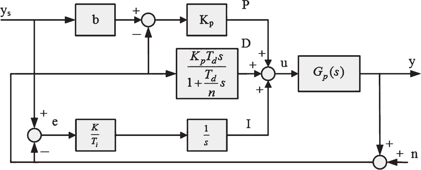
Refined PID Control.

$G (s) = \frac{K_{p} (b + \frac{1}{T_{i}} s) G_{p} (s)}{1 + K_{p} (1 + \frac{1}{T_{i}} s + \frac{T_{d} s}{(1 + \frac{T_{d}}{N} s)}) G_{p} (s)}$ (25) where G_p(s) is the transfer function of the plant.

3.2 ILC

Iterative Learning Control (ILC) combines artificial intelligence and control theory to create a controller with learning ability. Compared with traditional controllers, ILC does not require a complete dynamic model of the system, and it can also adapt well to variations in the environment.

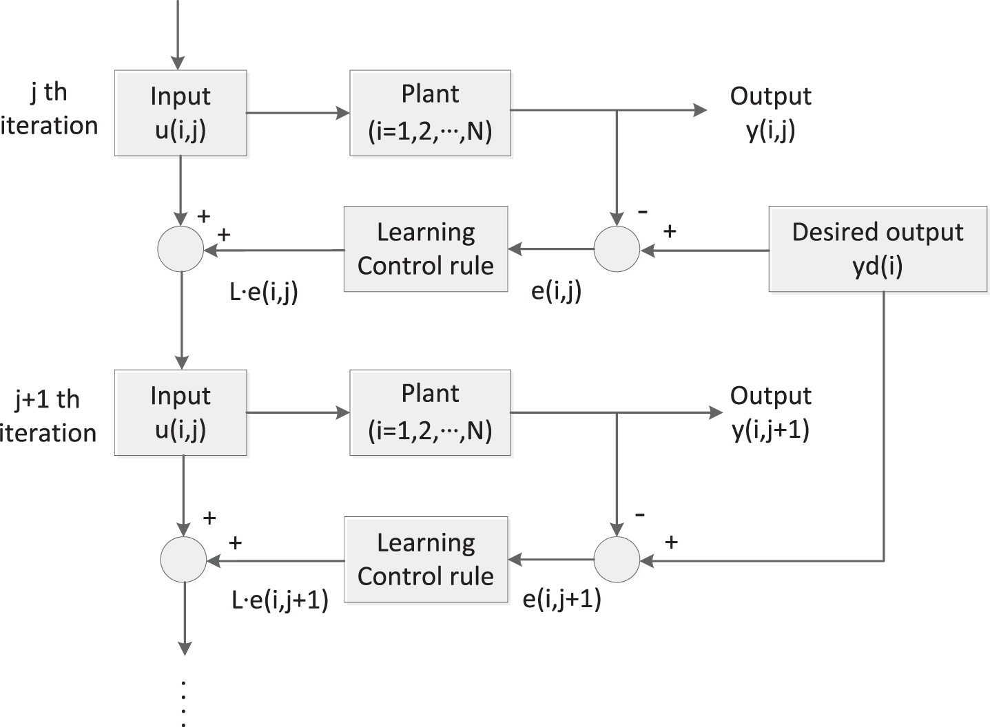
It is a good method of tracking control for a system which works in a repetitive mode. Repetition (iteration) allows the system to reduce tracking error from repetition to repetition, and the required input needed to track the reference exactly. Figure 7 depicts a typical ILC block diagram, the control law can then be expressed as $u_{j + 1} (i) = u_{j} (i) + {Le}_{j} (i)$ (26) where u_j(i) and u_j + 1(i) are the inputs, at time i, of iterations j and j + 1, respectively, L is the learning gain, and e_j(i) is the error of iteration j.

Fig. 7

ILC block diagram.

A linear, time invariant, and discrete time system, can be expressed by ${\begin{matrix} x_{j} (i + 1) = {Ax}_{j} (i) + {Bu}_{j} (i) \\ y_{j} (i) = {Cx}_{j} (i) \\ x_{j} (0) = x_{0} \\ i = 0, 1, \dots, M \\ j = 0, 1, \dots \end{matrix}$ (27) $lim_{j \to \infty} e_{j} (i) = lim_{j \to \infty} y_{d} (i) - y_{j} (i) = 0, i = 0, 1, . . ., M$ (28) where M is the upper bound of i, to be assigned by the designer.

There are various types of learning gains, one of them is the PID type [11, 12] which is widely used, and can be formulated as:

$\begin{matrix} u_{j + 1} (i) = u_{j} (i) + Δ u_{j + 1} (i) \\ i = 0, 1, . . ., M, j = 0, 1, . . . \end{matrix}$ (28) where Δu_j ₊ ₁(i) is a modified term. And the PID gains are specified as:

$\begin{matrix} Δ u_{j + 1} (i) = & k_{P} e_{j} (i + 1) + k_{I} \sum_{m = 1}^{i + 1} e_{j} (m) \\ + k_{D} (e_{j} (i + 1) - e_{j} (i)) \end{matrix}$ (29) where k_p, k_i, and k_d, are the real constants of proportional, integral, and derivative gains, respectively. In addition, $e_{j} (i) = y_{d} (i) - y_{j} (i), for 1 ⩽ i ⩽ M$ (30)

and $e_{j} (0) ≜ 0$ (31)

The optimal gains of k_p, k_i, and k_d are obtained by using the approach proposed by Madady [12]. The proposed procedure is outlined below.

From Equation (28), the following equation is easily obtained as $Y (j) = GU (j) + G_{0} x_{0}, j = 0, 1, . . .$ (32)

where U(j) and Y(j) are the input and output vectors, respectively, in iteration j, and can be expressed as $U (j) = {[\begin{matrix} u_{j} (0) & u_{j} (1) & \dots & u_{j} (M - 1) \end{matrix}]}^{T}$ (33) $Y (j) = {[\begin{matrix} y_{j} (0) & y_{j} (1) & \dots & y_{j} (M) \end{matrix}]}^{T}$ (34) In addition, $G = [\begin{matrix} g_{1} & 0 & 0 & \dots & 0 \\ g_{2} & g_{1} & 0 & \dots & 0 \\ g_{3} & g_{2} & g_{1} & \dots & 0 \\ ⋮ & ⋮ & ⋮ & ⋱ & ⋮ \\ g_{M} & g_{M - 1} & g_{M - 2} & \dots & g_{1} \end{matrix}]$ (35) and $G_{0} = [\begin{matrix} CA \\ {CA}^{2} \\ {CA}^{3} \\ ⋮ \\ {CA}^{M} \end{matrix}]$ (36) where the elements of G are the standard Markov parameters of the system, and can be obtained by $g_{k} = {CA}^{k - 1} B, k = 1, . . ., M$ (37)

Also, let H matrix be $H = [\begin{matrix} g_{1} & g_{1} & g_{1} \\ g_{2} & g_{1} + g_{2} & g_{2} - g_{1} \\ g_{3} & g_{1} + g_{2} + g_{3} & g_{3} - g_{2} \\ ⋮ & ⋮ & ⋮ \\ g_{M} & g_{1} + g_{2} + \dots g_{M} & g_{M} - g_{M - 1} \end{matrix}]$ (38)

Then $(H^{T} H)^{- 1} = [\begin{matrix} h_{1} & h_{2} & h_{3} \\ h_{2} & h_{4} & h_{5} \\ h_{3} & h_{5} & h_{6} \end{matrix}]$ (39)

The optimal parameters of the PID type ILC controller can be obtained as $k * = [\begin{matrix} k_{P}^{*} \\ k_{I}^{*} \\ k_{D}^{*} \end{matrix}] = [\begin{matrix} g_{1} (h_{1} + h_{2} + h_{3}) \\ g_{1} (h_{2} + h_{4} + h_{5}) \\ g_{1} (h_{3} + h_{5} + h_{6}) \end{matrix}]$ (40)

Finally, the sufficient condition for monotonic convergence is $ρ^{*} < M^{- 1}$ (41) where $ρ^{*} = 1 - g_{1}^{2} (h_{1} + 2 h_{2} + 2 h_{3} + h_{4} + 2 h_{5} + h_{6})$ (42)

4 Design example

The system model is found by the system indentification experiment, and can be expressed by $G (s) = \frac{V_{out} (s)}{V_{in} (s)} = \frac{1778}{s^{2} + 81.15 s + 1813} e^{- 0.0188 s}$ (43)

The inertial and dimensional parameters of the system is tabulated in Table 1. By substituting all the parameters into Equation (19), and set the nonlinear terms as f(t), it yields

Table 1

Inertial and dimensional parameters

Parameter	m₁(kg)	m₂(kg)	m₃(kg)	r(m)	l(m)	e(m)
Value	0.14	0.39	1.7	0.05	0.175	0.031

$m (θ) \ddot{θ} = f (t) + u (t)$ (44)

Where $u (t) = v (t) + u * (t) - f (t)$ (45) and u*(t) and v(t) are the outputs of ILC and PID controller, respectively. In addition, f(t) is expected to be eliminated by the compensation of the PID controller, then Equation (44) ca be expressed as $m (θ) \ddot{θ} = v (t) + u * (t)$ (46)

To simplify the system model, the time varying parameter M(θ) is replaced by its average value of one revolution, i.e., 1.591. Equation (46) can be simplified as $\ddot{θ} = [v (t) + u * (t)] / 1.591$ (47)

Let state variables(x₁, x₂) be $[\begin{matrix} x_{1} \\ x_{2} \end{matrix}] = [\begin{matrix} θ \\ \dot{θ} \end{matrix}]$ (48) and the output y(t) be $y (t) = x_{2} = \dot{θ}$ (49)

Then followed by substituting the parameters in Table 1 to Equation (19), the state equation of the system can be expressed as $[\begin{matrix} {\dot{x}}_{1} \\ {\dot{x}}_{2} \end{matrix}] = [\begin{matrix} 0 & 1 \\ - 7 . 5424 & - 9 . 428 \end{matrix}] [\begin{matrix} x_{1} \\ x_{2} \end{matrix}] + [\begin{matrix} 0 \\ 0 . 6285 \end{matrix}] u$ (50)

Substituting all the knowns and founds to Equation (37), the standard Markov parameters of the system can be obtained as

$g_{k} = {CA}^{k - 1} B = [\begin{matrix} g 1 \\ g 2 \\ g 3 \\ ⋮ \end{matrix}] = [\begin{matrix} 0.0057 \\ 0.0048 \\ 0.0042 \\ ⋮ \end{matrix}], k = 1, 2, . . ., M$ (51)

where M is set as 1000 by trial and error. Substituting Equation (50) into Equation (38), it yields $H = [\begin{matrix} 0.005529 & 0.005529 & 0.005529 \\ 0.004825 & 0.010355 & - 0.000703 \\ 0.004176 & 0.014532 & - 0.000648 \\ 0.003579 & 0.018112 & - 0.000596 \\ 0.003032 & 0.0211144 & - 0.000547 \\ 0.002531 & 0.023676 & - 0.000500 \\ ⋮ & ⋮ & ⋮ \end{matrix}]$ (52) and $(H^{T} H)^{- 1} = [\begin{matrix} 7745.0592 & - 4068.9064 & - 53.9751 \\ - 4068.9064 & 32698.6592 & 215.6513 \\ - 53.9751 & 215.6513 & 51.86348 \end{matrix}]$ (53)

Substituting Equations (50) and (53) into Equation (40), the optimal parameters can then be obtained as $k^{*} = [\begin{matrix} k_{P}^{*} \\ k_{I}^{*} \\ k_{D}^{*} \end{matrix}] = [\begin{matrix} 15.6287 \\ 159.0153 \\ 0.1343 \end{matrix}]$ (54)

By substituting k^*, g₁ and h_i (i = 1∼6) into Equation (41), we have $ρ^{*} = 4.6128 * 10^{- 7} < 1000^{- 1} (M^{- 1})$ (55)

Therefore, the monotonic convergence of the system is also assured.

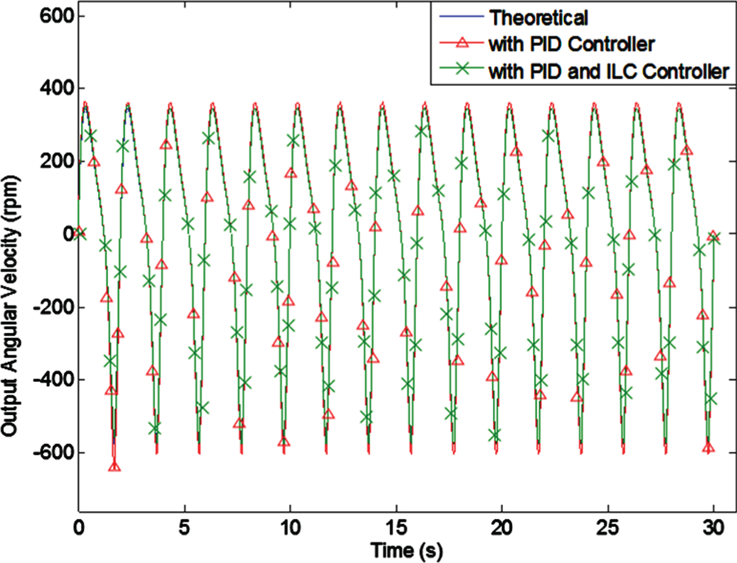
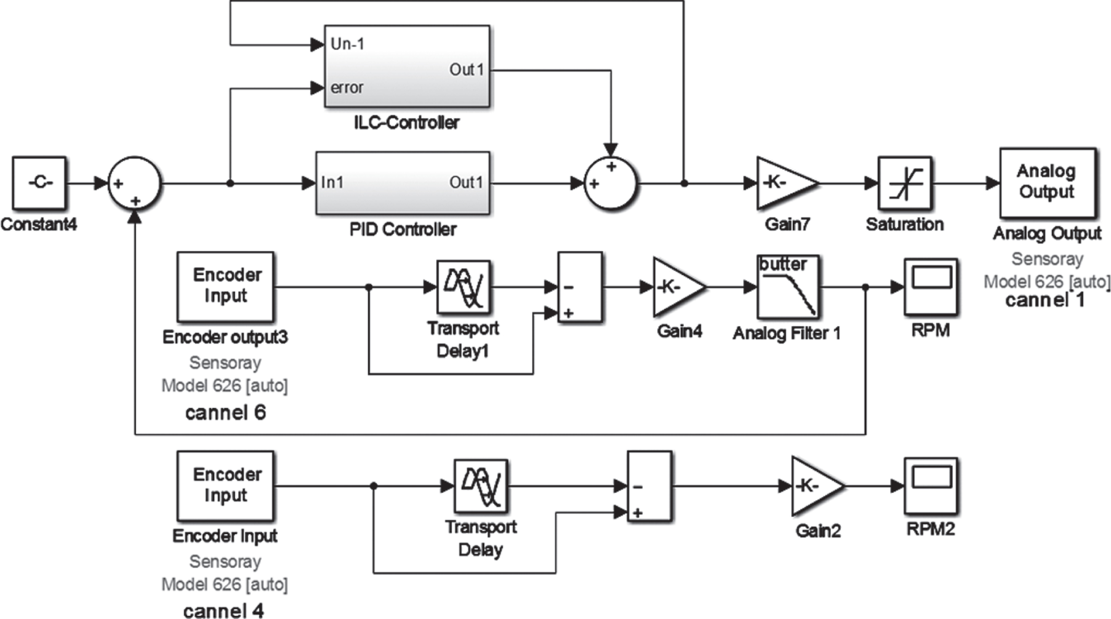
The design is simulated by using Simulink, Fig. 8 depicts the block diagram of the system, and the program is shown in Fig. 9. To verify the effectiveness of the design, the simulated result of the system with the hybrid controller is compared with the ones of the theoretical and with PID controller. Fig. 10 shows the output angular velocities during 0–30 secs with input angular velocity at 30 rpm, and the first two cycles are also depicted in Fig. 11, it can be found that the hybrid controller has significantly improved the tracking accuracy of the output in the first two cycles. In the 15th cycle, the output of the hybrid controller is almost coincident with the theoretical one, show in Fig. 12. The errors are presented in Table 2. The tracking accuracy of using the hybrid controller is better than that using the PID controller.

Fig. 8

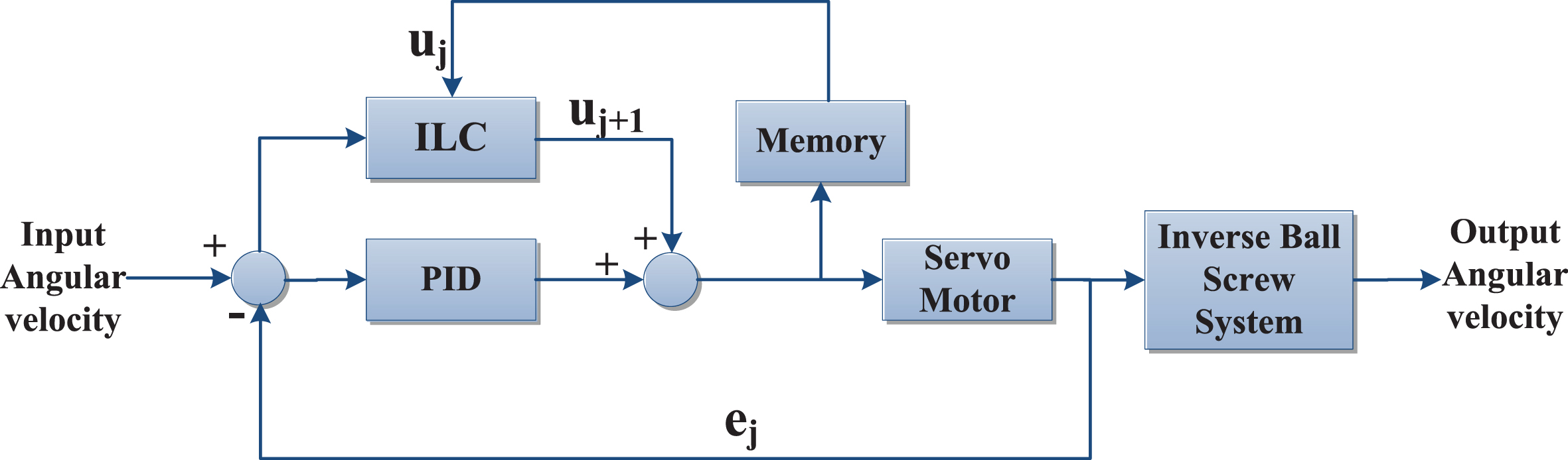
Block diagram.

Fig. 9

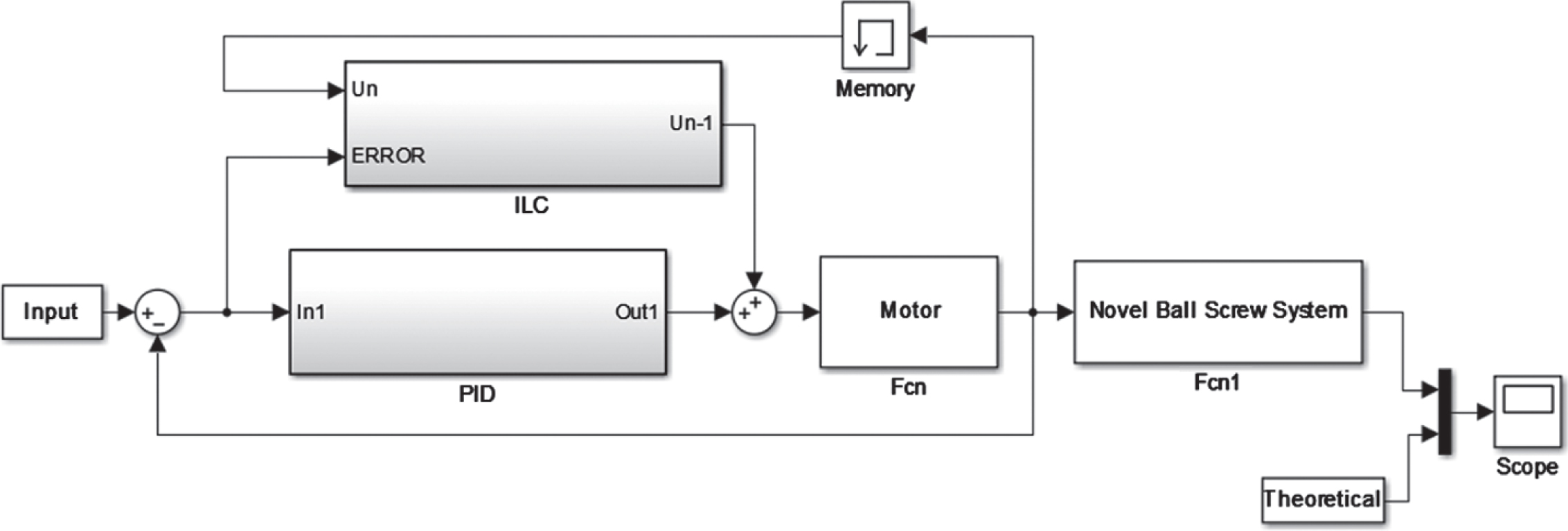
Simulink program (simulation).

Fig. 10

Output angular velocities (0–30 secs).

Fig. 11

Output angular velocities (1st & 2nd cycles).

Fig. 12

Output angular velocities (15th cycles).

Table 2

Output errors (simulation)

	PID controller	Hybrid controller
Square sum error (rpm²)	6.44×10⁶	1.24 ×10⁶
Improving percentage	90.65%	99.81%

5 Experiment

To investigate the discrepancy between the simulation and experiment, a prototype testing is conducted, as shown in Fig. 13. The specifications of the devices in the experimental setup are listed in Table 3.

Fig. 13

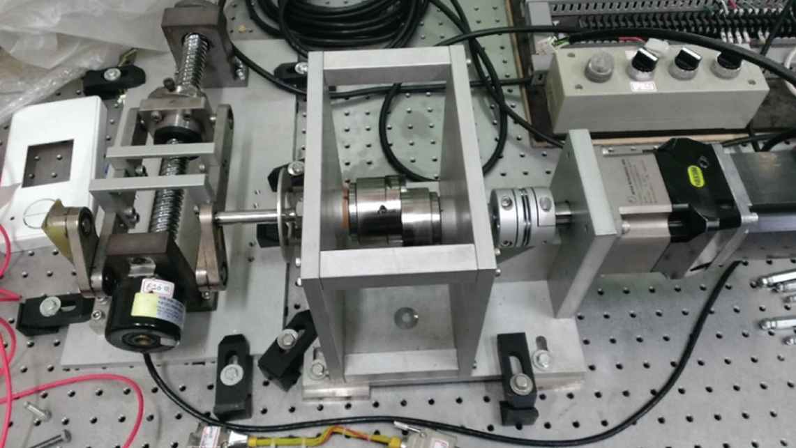
Experiment setup.

Table 3

Specifications

Name	Brand	Type
Servo motor	Mitsubishi	HC-KFS73(BG)
Servo driver	Mitsubishi	MR-J2S-70A
Gear reducer	Apex Dynamic	AB090-010-S2-P1
DAQ card	Sensoray	Model 626
Output encoder	Hontko	HTR-HM-12-900-3-L-M322

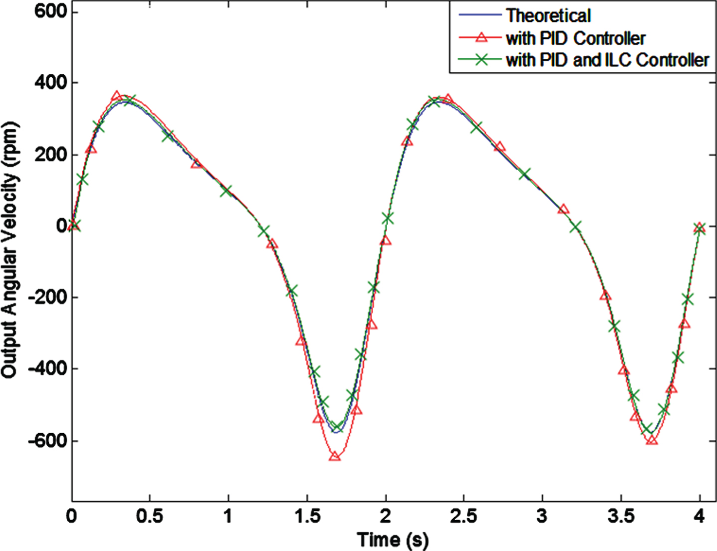
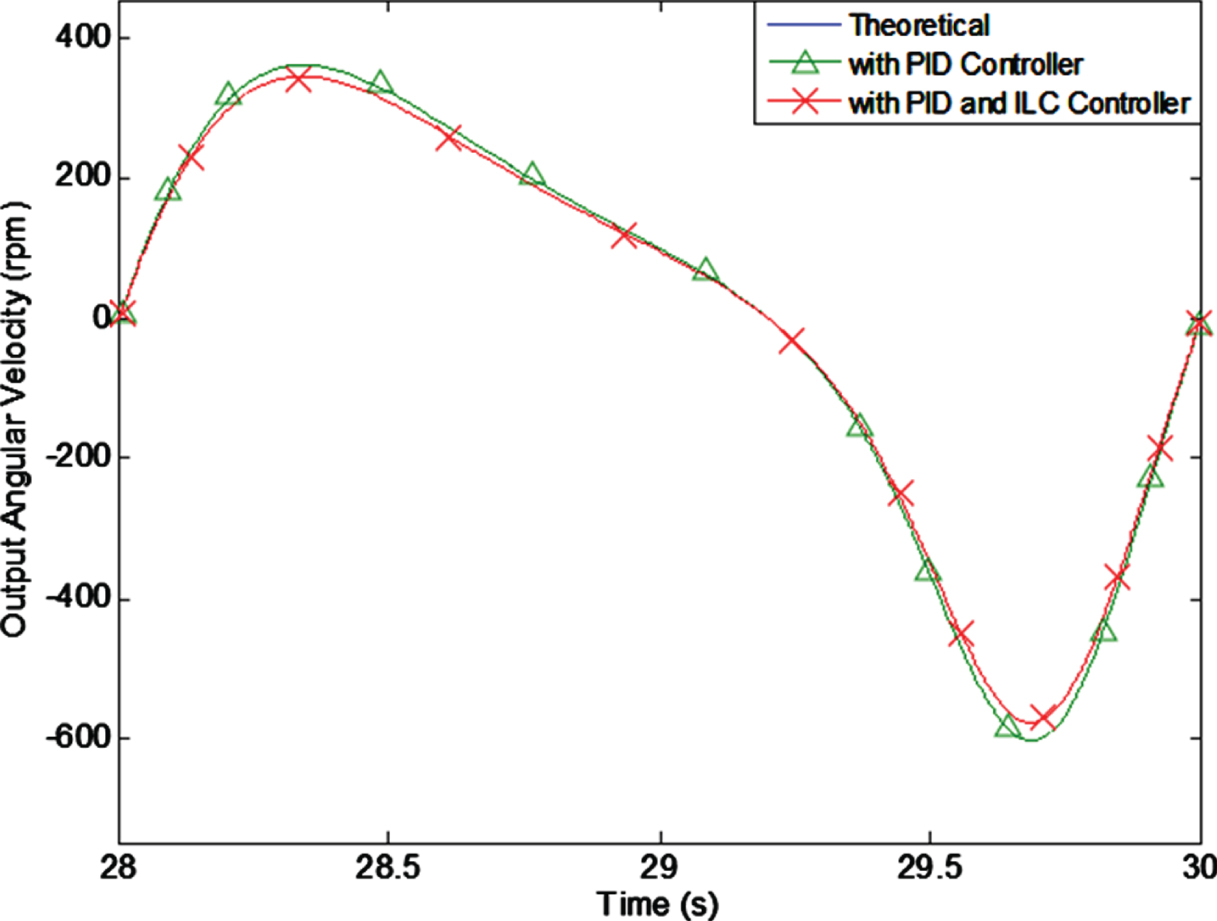
Figure 15 shows the comparison of the experimental output angular velocities of the theoretical, with PID controller, and with hybrid controller. The output angular velocity of using the hybrid controller is well track, at least roughly, the theoretical one. If the 1st and 2nd cycles are investigated, as shown in Fig. 16, it can be seen from the figure that the output in the 2nd cycle track better than that in the 1st cycle. In addition, Fig. 17 shows the comparison of the output angular velocity in various cycles. It can be found that the errors are gradually as the number of cycle increases, i.e., the cyclic error is reduced. Figure 17 show the output of the15th cycle, the square sum error is 2.41 × 10⁶, and 94.21% improvement compared to the output of no controller used. Although the improvement is a little smaller than the simulation one, but is still very high. Therefore, the proposed hybrid control can effectively reduce the tracking error.

Fig. 14

Simulink program (Experiment).

Fig. 15

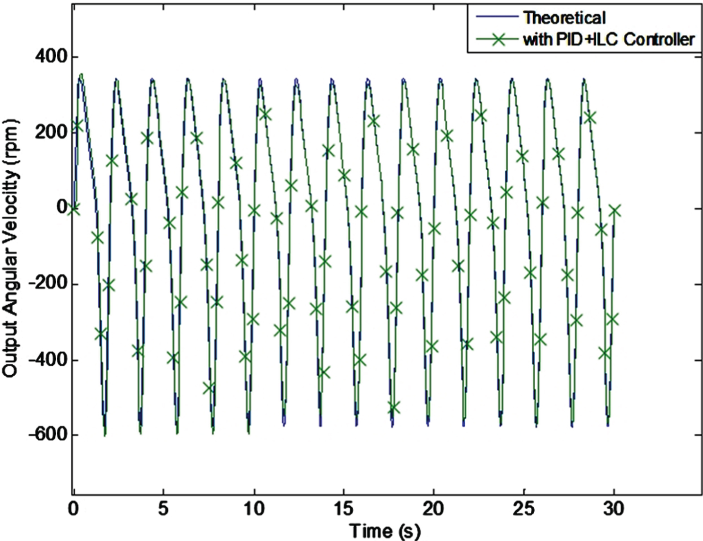
Experimental output angular velocity.

Fig. 16

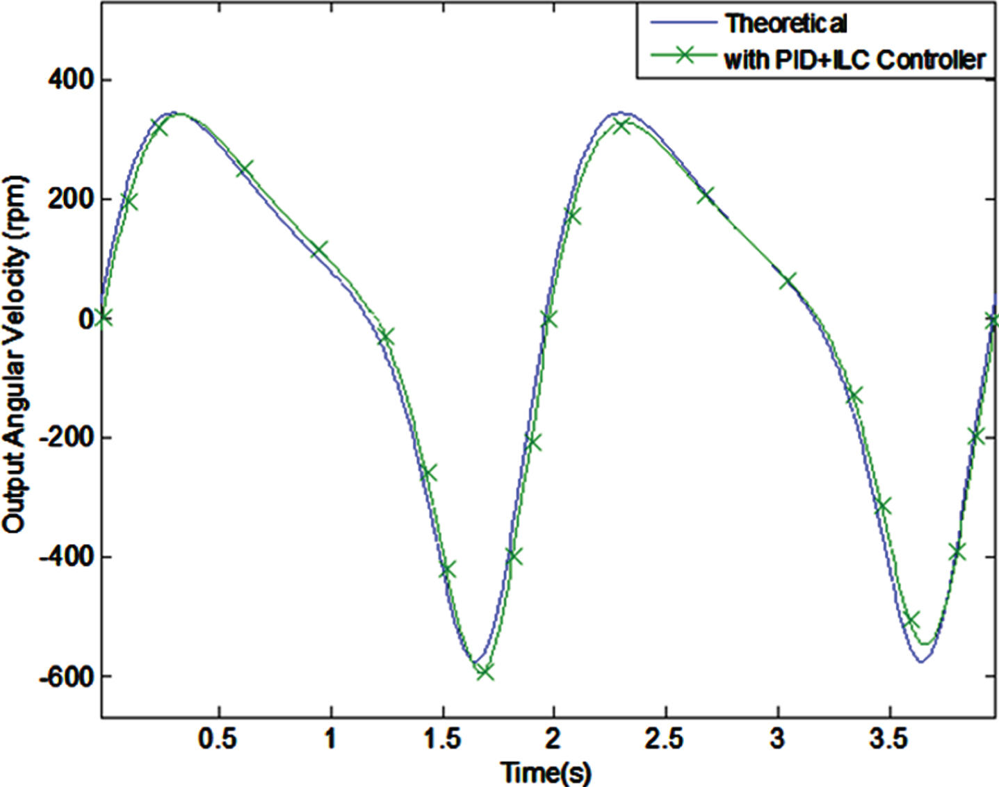
Experimental output angular velocity (1st & 2nd cycles).

Fig. 17

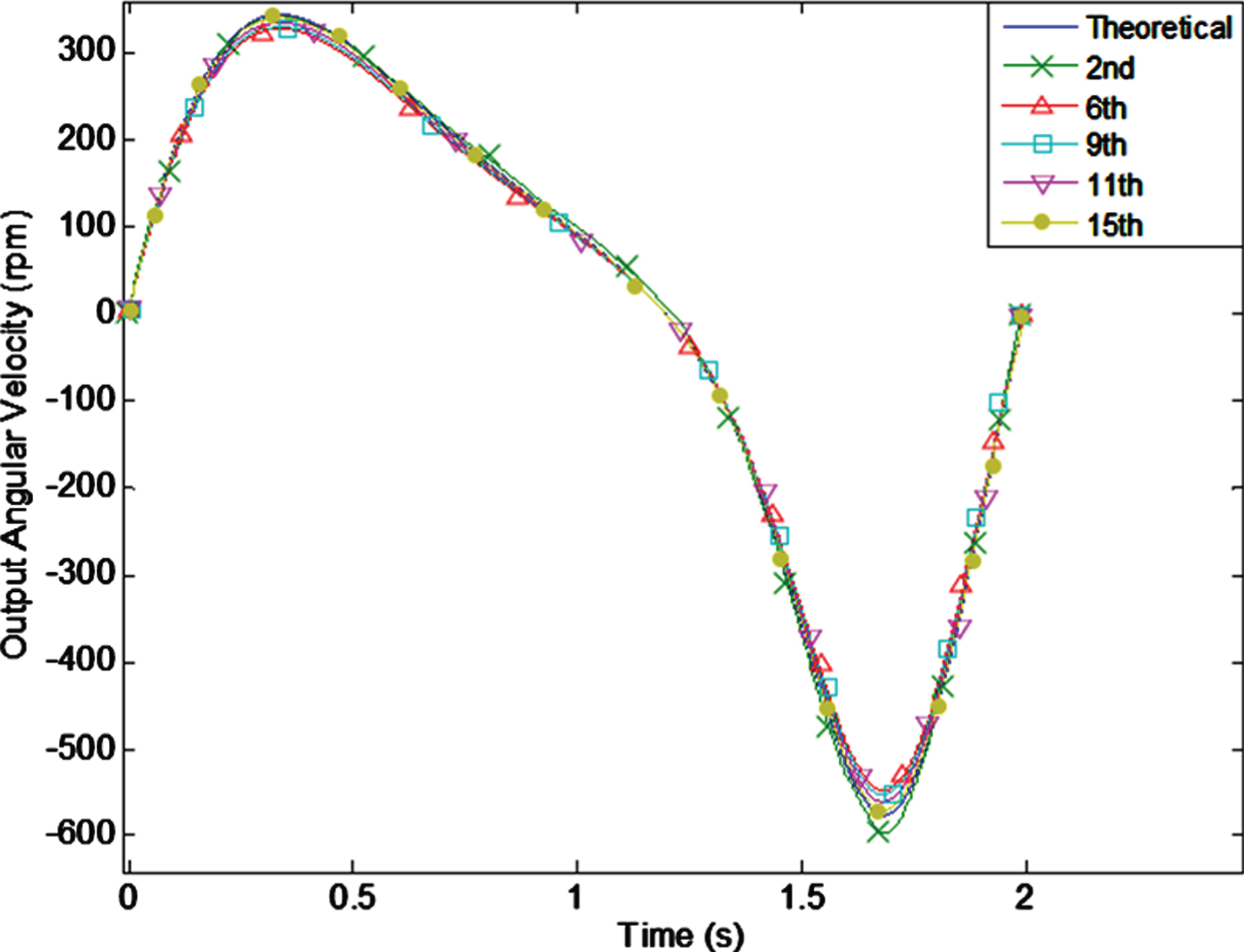
Experimental output angular velocity(15th cycle).

6 Conclusions

In this study, an approach for reducing the cyclic error of a ball screw transmission system has been proposed. Kinematic and dynamic analyses have been conducted. The model of the system has been formulated followed by the ILC controller design. The simulated and experimental results have shown that the proposed approach can further reduce the cyclic error. Therefore, the proposed approach is feasible and effective.

Footnotes

Acknowledgments

The support of the National Science Council, Republic of China (Taiwan), under Grants MOST 101-2211-E-150-037 and MOST 108-2637-E-150-001, is gratefully acknowledged.

References

Hsieh

W.H.

and Chang

K.B.

, Modeling and control of a novel ball screw mechanism, Journal of Marine Science and Technology 22 (2014), 754–761.

Niranjan

, Karinka

and Sairam

, Development of Precision Positioning Stage, Journal of Advanced Manufacturing Systems 18 (2019), 103–111.

Liu

, Quantitative analysis for effects of structural stiffness on vibration characteristics of machine tool feed system, Journal of Vibroengineering 22 (2020), 241–251.

Huang

Y.C.

and Chen

X.Y.

, Investigation of a ball screw feed drive system based on dynamic modeling for motion control, Advances in Technology Innovation 2 (2017), 29–33.

Abdulin

, Bolshakov

, Podshibnev

and Samsonovich

, Steering actuator based on a ball screw with a separator, IOP Conference Series: Materials Science and Engineering 862 (2020), 032082.

Liu

, Xu

and Zuo

, Design, modeling, lab, and field tests of a mechanical-motion-rectifier-based energy harvester using a ball-screw mechanism, IEEE/ASME Transactions on Mechatronics 22 (2017), 1933–1943.

, Chen

, Li

, Xu

, Liang

, Ngo

, et al., A compact mechanical power take-off for wave energy converters: Design, analysis, and test verification, Applied Energy 278 (2020), 115459.

Jin-qiu

, Zhi-zhao

, Lei

and Yu

, A review on energy-regenerative suspension systems for vehicles, in, Proceedings of the world congress on engineering 3 (2013), 3–5.

Nugraha

D.K.

and Guntur

H.L.

, Design and analysis of regenerative shock absorber using ball screw mechanism for vehicle suspension, AIP Conference Proceedings 2187 (2019), 050014.

10.

Uchiyama

, Formation of high-speed motion pattern of a mechanical arm by trial, Trans. SICE (Society for Implementation and Control Engineers) 14 (1978), 706–712. (In Japanese).

11.

Arimoto

, Kawamura

and Miyazaki

, Bettering Operation of Robots by Learning, Journal of Robotic Systems 1 (1984), 123–140.

12.

Madady

, PID type iterative learning control with optimal gains, International Journal of Control Automation and Systems 6 (2008), 194–203.

13.

Tan

K.K.

, Dou

and Yangquan

, High precision linear motor control via relay-tuning and iterative learning based on zero-phase filtering, IEEE Transactions on control systems technology 9 (2001), 244–253.

14.

Daley

, Hatonen

and Owens

D.H.

, Hydraulic servo system command shaping using iterative learning control, IEEE Int. UKACC Control 2004 Mini Symposia (2004), 117–121.

15.

Weizhe

, Panda

S.K.

, Masahiro

S.M.

and Xu

J.X.

, Torque ripple minimization in PM synchronous motors using iterative learning control, IEEE Transactions on Power Electronics 19 (2004), 1458–1463.

16.

Elci

, Longman

R.W.

, Phan

M.Q.

, Juang

J.N.

and Ugoletti

, Simple learning control made practical by zero-phase filtering: applications to robotics, IEEE Transactions on Circuits and Systems Fundamental Theory and Application 49 (2002), 753–767.

17.

Freeman

C.T.

, Cai

, Rogers

and Lewin

P.L.

, Iterative learning control for multiple point-to-point tracking application, IEEE Transactions on Control Systems Technology 19 (2011), 590–600.

18.

Matsushima

, Hashimoto

, Masahiro

and Fumio

, A learning approach to robotic table tennis, IEEE Transactions on Robotics 21 (2005), 767–771.

19.

Kim

D.I.

and Kim

, An iterative learning control method with application for CNC machine tools, IEEE Transactions on Industry Applications 32 (1996), 66–72.

20.

Tsai

M.S.

, Lin

M.T.

and Yau

H.T.

, Development of command-based iterative learning control algorithm with consideration of friction, disturbance, and noise effects, IEEE Transactions on Control Systems Technology 14 (2006), 511–518.

21.

Freudenstein

, Tsai

L.W.

and Maki

E.R.

, Generalized Oldham Coupling, Journal of Mechanisms Transmissions and Automation in Design 106 (1984), 475–481.

22.

Hsieh

W.H.

and Tsai

C.H.

, A study on a novel quick return mechanism, Transactions of the Canadian Society for Mechanical Engineering 33 (2009), 487–500.

23.

Hsieh

W.H.

and Tsai

C.H.

, On a novel press system with six links for precision deep drawing, Mechanism and Machine Theory 46 (2011), 239–252.

24.

Hsieh

W.H.

, A study on a novel ball screw transmission system, Master Thesis, Institute of Mechanical & Electro-Mechanical Engineering, National Formosa University, (2008).

25.

Crespo da Silva

, Intermediate dynamics for engineers: complemented with simulations and animations, 1st edition, McGraw Hill, (2014).

26.

Astrom

K.J.

and Hagglund

, PID controllers: theory, design and tuning, Instrument Society of America, Research Triangle Park, North Carolina, (1995).