Fuzzified time-frequency method for identification and localization of power system faults

Abstract

In this work, different types of power system faults at various distances have been identified using a novel approach based on Discrete S-Transform clubbed with a Fuzzy decision box. The area under the maximum values of the dilated Gaussian windows in the time-frequency domain has been used as the critical input values to the fuzzy machine. In this work, IEEE-9 and IEEE-14 bus systems have been considered as the test systems for validating the proposed methodology for identification and localization of Power System Faults. The proposed algorithm can identify different power system faults like Asymmetrical Phase Faults, Asymmetrical Ground Faults, and Symmetrical Phase faults, occurring at 20% to 80% of the transmission line. The study reveals that the variation in distance and type of fault creates a change in time-frequency magnitude in a unique pattern. The method can identify and locate the faulted bus with high accuracy in comparison to SVM.

Keywords

Power system faults localization identification fuzzy logic signal processing

1 Introduction

Till date various researchers had dealt the subject of identification of power system faults using both parametric and non-parametric methods. The researchers had purposely used these techniques for extracting the features of any given signal. Parametric methods include ESPIRIT, MUSIC, ARMA, Auto-Regressive, Prony analysis, whereas Non-parametric methods include analysis based on Signal Processing methods. Non-parametric approaches were also adopted by many researchers for the identification of power quality events. The techniques like Wavelet Transforms, Stockwell Transforms, and Gabor-Wigner transform, and modified versions of these techniques were used to identify the type of power quality event.

However, these techniques alone were not enough to identify or classify the type of power system disturbance, particularly the transients. The features obtained using the signal processing methods need to be fed to any artificial intelligence module for automatic classification. A lot of research has been reported in the literature in the area of artificial intelligence techniques for power system protection. The major problem statements in the power system is the identification and location of disturbances originating due to various sources such as malfunctioning equipment, system faults, nonlinear loads and others. However, identification of the type of power system faults and locating them is one of the significant tasks. Also, due to the system interconnection, makes it more challenging to identify the origin of faults. Hence, a comprehensive system which can identify and locate the power system faults rapidly with high accuracy is needed. Such requirement had led the authors to propose a system that can identify and locate the origin of such events at an early stage before the faults hamper the regular power system operation [1].

In the past, power system faults have been classified and identified using Wavelet Transform (WT) and Stockwell Transform (ST) and is evident in the literature [2 –7]. However, the application was limited to the generation of unique signatures only, and these are the visual identification process in which a high technical knowledge about the transformation techniques is required [8]. Further, the power system faults were identified using an artificial intelligence technique wherein the input waveforms are generated using mathematical equivalents and not from a non-standard power system model.

The researchers in [9 –11] have presented a methodology to classify and identify various power transients, including faults but these works are silent about the location of power system faults. Another dimension which was left unexplored in these works is that the Continuous ST plots of faults give similar signatures visually though the matrix values are different, wherein the primary reason being minute variations in the plot for various transients. Such features of the Time-Frequency resolution techniques make it unfit for faults analysis if the features are not effectively utilized. In such a case, unique indices or parameters need to be designed based on which a fault can be identified and located.

Since the severity level of the Symmetrical and Unsymmetrical faults cannot be generalized and classified based on the short circuit current magnitude, recognition of faults poses a difficult task. As age has advanced, a modified and Inverse version of the Stockwell transform were also proposed [12 –15]. These inverse S-Transform techniques, along with various properties of Discrete ST, have also been used to extract unique identification features and identify accordingly [16].

Few researchers have also used Fuzzy logic, Support Vector Machine (SVM), Artificial Neural Network (ANN) and other Artificial Intelligence (AI) techniques along with signal processing for power system faults recognition. The authors in [17] have proposed an ANN-based method for identification of the type of fault in a two-generator power system, where the carried out work is limited to only identification with two generator model. Fault identification and localization using Phasor Measurement Unit (PMU) with SVM classifier were proposed in [18] wherein a two-generator system was considered, the Fast Fourier Transform (FFT) coefficients up to 4th harmonics are used to extract the identification parameters. Further, researchers in [19] have proposed a Continuous Wavelet Transform (CWT) and ANN to identify and locate the type of fault in a multi-bus system. However, the length of the transmission line considered is minimal, and only one generating station is considered. Also, the generator is not assumed to inject any magnitude of harmonics which makes the case simple. Petrinet based method was also proposed in [20], but the application was restricted to the zoning of faults only. Further, authors in [21 –23] had proposed ANN, Fuzzy and SVM approach for identification of faults. However, the noise effect was not considered, and computational time has not been discussed.

Hence, still, there is an inescapable requirement of advanced prediction techniques, which can rapidly identify and locate various power system faults in an interconnected multi-generator power system. This requirement forms the motivation of this article to propose a novel methodology for rapid auto-identification of power system faults. In this paper, unique features extracted from the area of the Gaussian window dilation of S-transform have been used to feed the fuzzy tree, which correctly predicts the power system faults. Few more environmental variables have been introduced to increase the complexity of the problem statement. It has been achieved by adding the parameters like harmonic injection in the source side, voltage unbalance, and frequency variations. The results obtained from the proposed methodology are more beneficial and fast in comparison to the techniques discussed earlier as it can detect the type as well as the fault location.

1.1 Novelty of the work

As mentioned above a signal processing based Fuzzy system has been proposed for classification of the nonlinear loads. Though there are many articles which had reported results with the highest accuracy, there are few areas which are improved and addressed in this article. These are listed as below: -

Power system faults in an interconnected power system have been considered. Till date, much research was done in fault waveform obtained from two generator systems or a mathematical equivalent of various faults. However, power system faults in the interconnected power system are less explored.

Power system faults occurring at various distances have been considered for identification, including the effect of source-side harmonics.

An accuracy of 99.24% has been reported, which is very high with minimal features and computationally lighter design.

With these points, it is mentioned here that this article will add more value to the literature and bridges the unexplored gaps in the area of power system fault identification. This paper is organized into six sections, including the introduction. The models considered for implementing the proposed methodology is explained in detail in Section 2. The methodology is presented in Section 3, and Section 4 provides the particulars of the designed fuzzy system. The identification results are presented in Section 5. Finally, conclusions are drawn in Section 6.

2 IEEE-9 Bus and IEEE-14 Bus test models

For verification of the proposed method, a standard IEEE-9 and IEEE-14 Bus power systems are considered for simulation. All the waveforms are obtained through these simulated models only. It is ensured that the system parameters are as defined by the IEEE working group. In this work, both types of faults, i.e. symmetrical and unsymmetrical faults, have been simulated. The fault inception length and locations have been varied to obtain waveforms at all the three recording stations, i.e. at Bus no. 4, 7 & 9 in the IEEE-9 Bus system. The faults are created between Bus 4 & 5, Bus 8 & 9 and Bus 7 & 8.

In the case of IEEE-14 Bus system, it is observed that Bus No. 2 and Bus No. 13 are having a greater number of connections with other buses, i.e. the impedance matrix of Bus 2 and Bus 13 are less sparse. Hence, faults between Bus 2 & 1, Bus 2 & 3, Bus 2 & 4, Bus 2 & 5, Bus 13 & 14, Bus 13 & 12 and Bus 13 & 6 have been considered for identification and location. In total, seven (07) combinations have been simulated. For both IEEE-9 Bus and IEEE-14 Bus, faults at a distance of 20%, 40%, 60% and 80% from the source have been considered for identification.

The system, as shown in Fig. 1 is an IEEE standard nine bus system with the impedance and voltage values mapped to the scale of 230 kV with 100 MVA as the base. In case of IEEE-14 Bus, the respective voltages defined by the IEEE working group for various buses along with the MVA ratings have been scaled to maintain PU value. Two systems with different unit base, i.e. per-unit and SI units are considered to standardize the proposed methodology for any voltage level. The locations have been kept unchanged for both the generators and connected loads. However, in both cases, the magnitudes of voltage and current are normalized before feeding to the algorithm.

Fig. 1

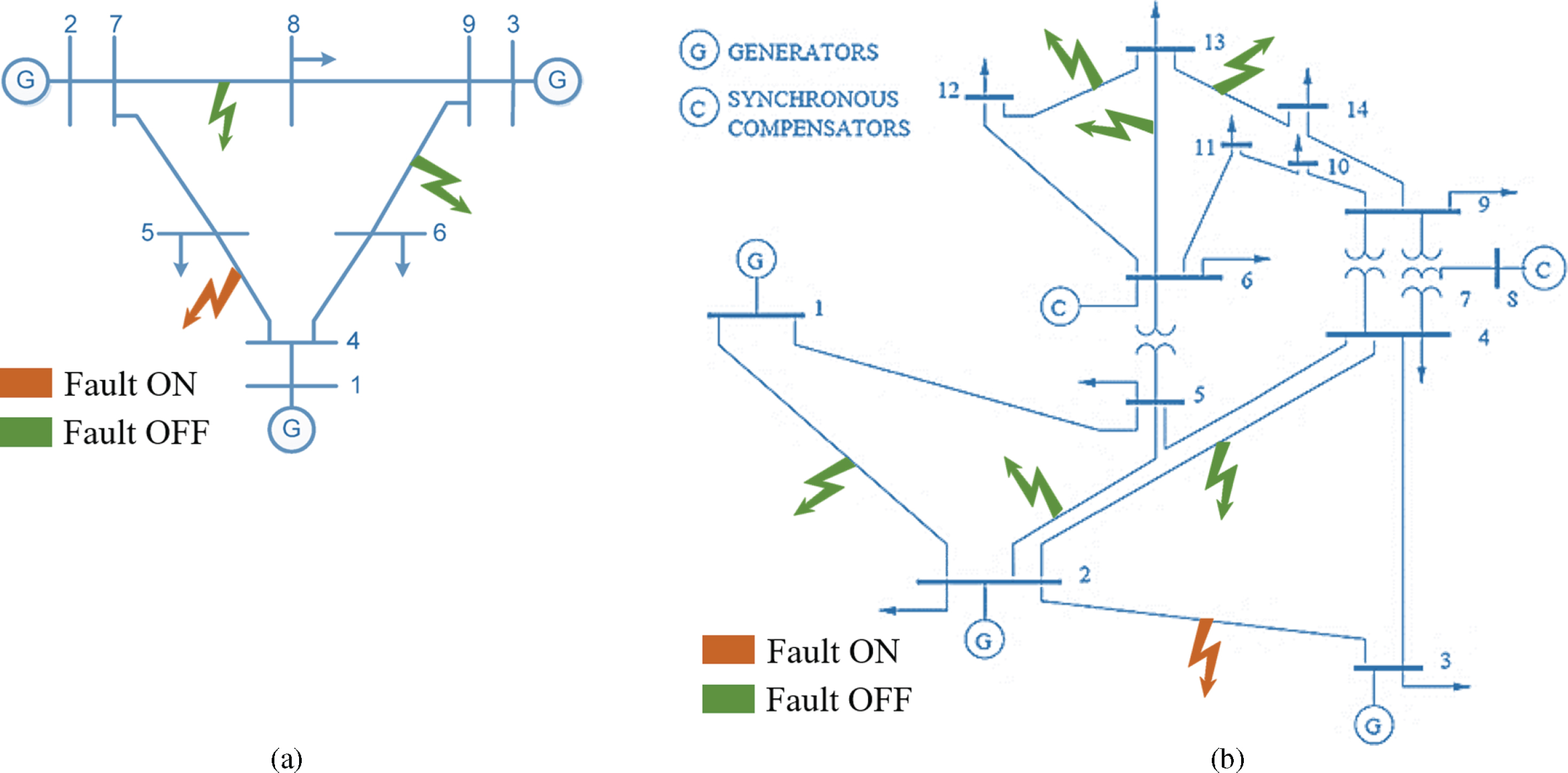
Standard (a) IEEE 9-Bus and (b) IEEE 14-Bus systems simulated for obtaining the power system current data.

In order to simulate different real-time problems, the below mentioned assumptions have been considered:-

At any time, different types of faults may occur, and the fault inception may be at any distance from the recording substation. However, one kind of fault occurs at any one location, as indicated in Brown and Green color in Fig. 1. The brown color is the instant when a fault occurs in a particular location and no fault at the other areas, which is shown in Green.

Since real-time data may contain noise due to measurement devices, surroundings, and other factors, a Gaussian noise of 30 dB standard limits has been added.

By considering the above factors, a calculated effort has been put to achieve the real-time behavior. Initally the sampling frequency is set at 5 kHz to include majority of the transient variations for identification. The recorded signals were then converted into per-unit values and retained for further analysis and identification in database experiment wise. MATLAB^®/SIMULINK is used to obtain the input waveforms [24].

Three (03) types of power system faults are considered for testing which are mentioned as under:-

Symmetrical Faults,

Asymmetrical Phase Faults, and

Asymmetrical Ground Faults.

These types of faults may act at any location on the line varying from 20 to 80% of the T/m line length from the busbar, i.e. the substation. Each class is defined using the type of fault along with the location i.e. for total three types of faults and four locations a total of twelve (12) classes are defined. Table 1 lists all such classes used in this work for classification.

Table 1

Class, Type of fault and Variable defined for identification

Class	Type of simulated fault	Variable Name
1	Symmetrical Fault at 20% length	F1
2	Symmetrical Fault at 40% length	F2
3	Symmetrical Fault at 60% length	F3
4	Symmetrical Fault at 80% length	F4
5	Asymmetrical Phase Fault at 20% length	F5
6	Asymmetrical Phase Fault at 40% length	F6
7	Asymmetrical Phase Fault at 60% length	F7
8	Asymmetrical Phase Fault at 80% length	F8
9	Asymmetrical Ground Fault at 20% length	F9
10	Asymmetrical Ground Fault at 40% length	F10
11	Asymmetrical Ground Fault at 60% length	F11
12	Asymmetrical Ground Fault at 80% length	F12

For each class, measurement has been taken from three substations, i.e. at Bus No. 4, 7 & 9 in IEEE-9 Bus system and Bus 2 & 13 in IEEE-14 Bus system with variations in the occurrence of a fault, inclusion of generation side harmonics, and unbalance. In totality, 108 sets of recordings have been done using nine (09) sets for each of the twelve classes i.e. 12 × 9 = 108 sets for IEEE-9 Bus and IEEE-14 Bus systems. Among 108 recordings, 36 recordings (randomly chosen three recordings from each class) have been used for training, another set of 36 recordings have been used for validation and remaining 36 have been utilized for independent testing of the proposed system. This set of data is generated for all the three cases of IEEE-9 Bus, i.e. the faults between Bus 4-5, Bus 8-9 and Bus 7-8 and seven (07) cases of IEEE-14 Bus system, i.e. the faults between Bus 2.1, Bus 2-3, Bus 2-4, Bus 2-5, Bus 13-14, Bus 13-12 and Bus 13-6.

3 Method adopted

The methodology used for identifying and locating the type of fault in the IEEE 9 & 14 Bus power system mentioned above is discussed in this section. A flowchart is shown in Fig. 2 for more natural interpretation. The description about each stage of Fig. 2 is provided in further subsections.

Fig. 2

Flowchart showing the steps involved in identification and localization of power system faults.

3.1 Signal conditioning

For detection of zero crossings in the reference supply signal, a suitable 50 Hz bandpass filter has been applied on the buffered signal, during the simulation. The detection of zero crossings is required to monitor any abnormal changes within the next zero crossings in a half cycle. Any abnormality beyond the defined limits triggers the proposed algorithm and identify the type and location of the fault. After that, three (3) complete cycles of the actual voltage are extracted for further processing, which acts as a reference supply signal. These three cycles are then transformed into the time-frequency domain using the Stockwell transform (ST), thus completing Steps 1 & 2 of Fig. 2.

3.2 Theory of stockwell transform (ST)

The continuous S transform (CST) as defined in [8 –13] is shown below

$\begin{matrix} S (τ, f) = & \int_{- \infty}^{+ \infty} h (t) (\frac{| f |}{\sqrt{2 π}} . exp (- \frac{{(t - τ)}^{2} f^{2}}{2}) . \\ exp (- (i 2 π ft)) . dt \end{matrix}$ (1) and the width of the Gaussian window is $σ = \frac{1}{| f |}$ (2)

The Gaussian window is chosen because it is the most compact in time and frequency, as mentioned by Stockwell transform in [5]. The Discrete S–Transform (DST) of Equation (1) is a representation of the local spectra, which can be obtained by the shift operation on the Fourier spectrum and is expressed as Eqnuation (3),

$\begin{matrix} S [kT, \frac{n}{NT}] \\ = \sum_{k = 0}^{N - 1} H [\frac{m + n}{NT}] . e^{\frac{- 2 π^{2} m^{2}}{n^{2}}} e^{\frac{i 2 π mk}{N}} for n \neq 0 \end{matrix}$ (3) where k, n, m = 0 .... N-1, T = Sampling time and N = Number of samples [8, 13].

It is known that S-Transform does localization of both phase and amplitude spectrum. The Gaussian window defined in ST varies with both time and frequency of the input signal. Due to such definition ST maintains good time and frequency resolution. The power system signals being non-stationary, S-trans form can effectively be applied. Next section discusses the extraction of discriminatory features of ST matrix coefficients obtained from Equation (3) for identification of power system faults. This completes Step 3 of Fig. 2.

3.3 Feature extraction

Since the response of the ST is exclusive for each type of fault, the ST matrix values, as shown in Equation (3) have been used for the parameter extraction. The properties of the ST matrix are as indicated below in Fig. 3. The ST matrix contains the responses at various time and frequencies, which are known as locals and voices. A local is obtained when the time is constant with variable frequency, and a voice is a variation in response to the change in time at a constant frequency. Both these properties of a time-frequency matrix provide much useful information. A local gives the information about variations in amplitudes at any instant of time, and a voice offers the information of variation in amplitudes at a frequency of interest. The same is demonstrated in Fig. 3(a) & 3(b) with ST plot of a sample power system disturbance. For a pure sinusoidal signal, the maximum values of the locals at any time are the same, and the voices are same beyond the fundamental frequency, as there are no additional frequency components/magnitude disturbances.

Fig. 3

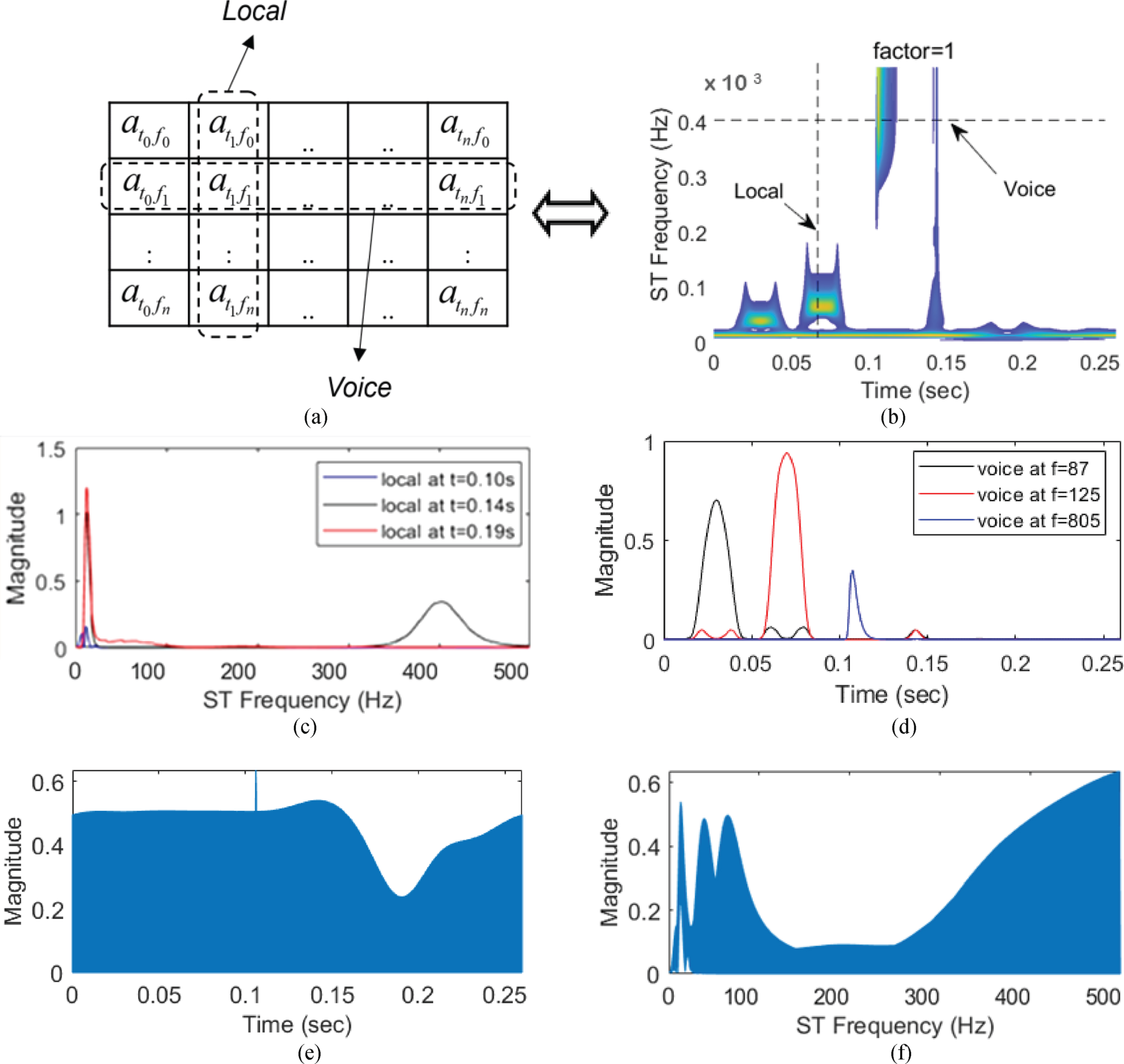
Elements of ST matrix with definition of Voice and Local. (a) ST matrix formation (b) Representation of the ST response plot as defined in Equation (1) (c) Locals at various intervals (d) Voices at various frequencies (e) shaded area under the curve of maximum values of all locals (ACM) (f) shaded area under the curve of maximum values of all voices (ARM).

However, the maximum values of locals and voices will not be the same for power system disturbances due to the presence of various frequencies with corresponding magnitudes. Hence, these maximum values of each local and voices naturally contain essential information of the type of power system disturbances. The plot of highest magnitudes of all locals vs time, i.e. the maximum values of columns of ST matrix in Fig. 3(b) vs ST time (CM) and plot of highest magnitude of all voices in Fig. 3(b) vs frequency, i.e. the maximum values of all rows of ST matrix vs ST frequency (RM) provide the information of the variations of an input signal.

The locals and voices at various time and frequency occurrences of the ST matrix in 3(b) are shown in Fig. 3(c) and 3(d). These locals and voices indicate the presence of other frequency components and magnitude variations. Figures 3(e) & 3(f) are the area plot of the maximum values of each local and voice of the ST matrix. There are variations in the magnitudes of RM plot, where the reoccurrence of the peak is due to the events like voltage regain after an interruption, at 0.2 s in Fig. 3(e). Whereas, the area under the maximum values of each voice indicates the presence of multiple peaks, i.e. high-frequency components. The area under these CM and RM plots have been used as the features for identifying and locating the power system faults in the considered IEEE systems. Below mentioned are the parameters defined for identification of the nature and location of power system faults. $\begin{matrix} ACM = & Area [Max . values of Locals of \\ ST matrix] \end{matrix}$ (4) $\begin{matrix} ARM = & Area [Max . values of Voices of \\ ST matrix] \end{matrix}$ (5)

The area is obtained using the MATLAB^® function trapz with the y-axis being the ST Magnitude and x-axis either being ST Time or Frequency. The features, i.e. the values of ARM and ACM are obtained for a different type of faults at different distance of occurrence, i.e. 20%, 40%, 60% & 80% of the T/m line length and recorded at Bus 4, Bus 7 and Bus 9 in IEEE-9 Bus system and Bus 2 and Bus 13 in IEEE-14 Bus system. This completes Steps 4 & 5 of Fig. 2.

4 Fuzzy rule based classification

For identifying the type and location of fault, a fuzzy logic classifier has been designed along with cusotmised rules and membership functions. Though many artificial intelligence algorithms are available, a fuzzy classifier is chosen because it easier in implementation and doesn’t require much hardware configurations. The proposed method in section provides a unique range of values for all the cases and giving these values to a Fuzzy rule base helps in fast, accurate and automatic identification. The area of overlap of membership functions and the rule base was chosen according to the range of each type of faults. Mamdani type fuzzy classifier has been used with Intuition method to determine the values of the triangular membership functions. The centroid approach was adopted for defuzzification. The Fuzzy system’s cumulative structure has been graphically shown in Fig. 4. Some random samples are fed for testing the robustness and precision of the designed fuzzy system. The obtained ARM & ACM values are provided to the fuzzy classifier to identify the type & location of fault based on the rules. This completes the final steps 6 & 7 of Fig. 2.

Fig. 4

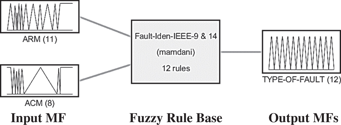
A high-level fuzzy classification system used for location and type of fault.

5 Results and discussion

This section presents the obtained results with the methodology explained in section 3. All Symmetrical and Asymmetrical Faults have been considered at 20%, 40%, 60% and 80% at from Bus 4, Bus 7 and Bus 9 in IEEE-9 Bus system and Bus 2 & 13 in IEEE-14 Bus system with Seven (07) combinations as mentioned previously. The ST plot for AB fault at 60% of the t/m line length along with the recorded voltage, ARM and ACM plots is shown in Fig. 5 to demonstrate the performance of ST. The recorded fault voltage at Bus 9 has been analyzed through ST defined in Equation (3) and is shown in Fig. 5(a). It is observed that the time-frequency plot reveals much information about the magnitude and frequencies present in the voltage.

Fig. 5

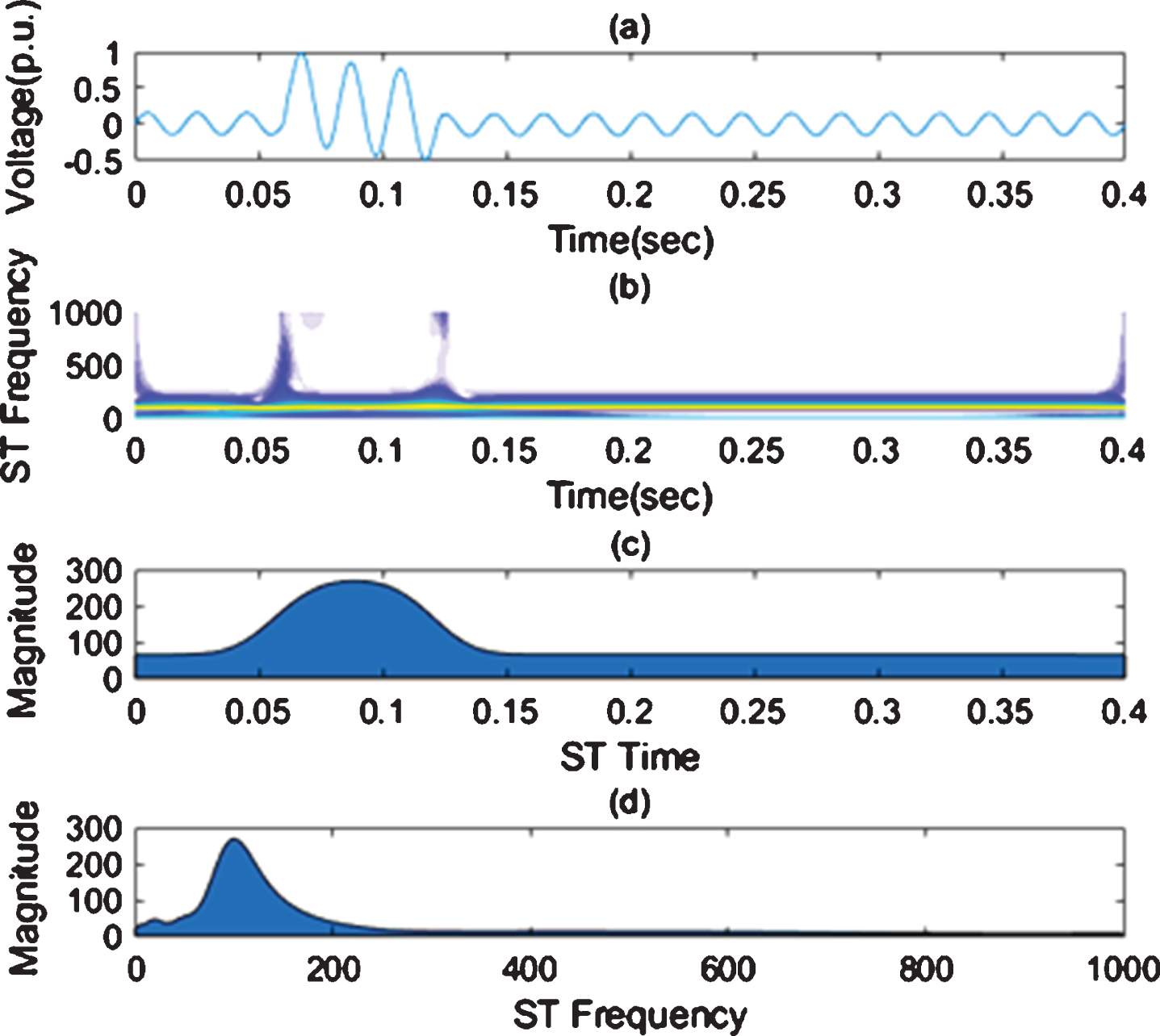
(a) Voltage waveforms recorded at Bus 9 along with the (b) ST plot, (c) ACM Plot and (d) ARM plots for AB fault at distance of 60% of the length of t/m line from Bus 6.

Using this ST plot complete data set has been obtained for all fault cases. Further, the proposed ARM and ACM parameters have been extracted, which vary dynamically with various types of faults which also varies with the nature of fault inception. During the study of the same, it was observed that there is a variation in fault behavior due to the following factors: -

effect of power swing generating source and

effect of angle/time of inception of fault.

These factors have caused a change in the fault behavior and thus in the extracted parameters also, i.e. in ARM and ACM. The results obtained for both IEEE-9 and IEEE-14 bus systems are discussed in the consecutive paragraphs.

5.1 IEEE-9 Bus system

The features of ACM and ARM have been extracted and presented in Table 2. The area of ARM is at a higher range in comparison to ACM as the x-axis for calculating ARM is the frequency which is varying from 50 to 2000 Hz. In contrast, the x-axis for ACM is the time in seconds, i.e. t = 0.0218 to 0.0818 s, leading to low value with decimals.

Table 2
Area under the Envelope of Maximum Value of Each Row of ST Matrix w.r.t Frequency for Different cases of Faults

Fault between Data recorded at Distance of Fault inception from Data recorded Bus (in %) Area of envelope of Maximum values of Rows (ARM) for different type of faults Area of envelope of Maximum values of Columns (ACM) for different type of faults

LLL LLG LL LLL LLG LL

Bus 4-5 Bus 4 20 30568 18152 11254 0.9408 0.8917 1.4804

40 25670 13004 10704 0.9846 0.9399 1.4939

60 17710 9862.90 10423 1.0438 1.0039 1.5081

80 10490 6929.10 8277 1.0963 1.0606 1.5226

Bus 7-8 Bus 7 20 26538 17649 11237 0.9579 0.9163 1.4964

40 20841 12863 10530 0.9716 0.9228 1.5076

60 15260 13133 9561.7 1.0161 0.9711 1.5188

80 13080 11593 9667.7 1.0603 1.0202 1.5308

Bus 8-9 Bus 9 20 24457 14606 11803 0.9602 0.8954 1.5118

40 17587 12185 9982 0.9901 0.9424 1.5214

60 13024 7402.80 10422 1.0407 1.0045 1.5326

80 9060.20 6642.40 10172 1.0841 1.0571 1.5440

Fault between	Data recorded at	Distance of Fault inception from Data recorded Bus (in %)	Area of envelope of Maximum values of Rows (ARM) for different type of faults	Area of envelope of Maximum values of Columns (ACM) for different type of faults
Bus 4-5	Bus 4	20	30568	18152	11254	0.9408	0.8917	1.4804
		40	25670	13004	10704	0.9846	0.9399	1.4939
		60	17710	9862.90	10423	1.0438	1.0039	1.5081
		80	10490	6929.10	8277	1.0963	1.0606	1.5226
Bus 7-8	Bus 7	20	26538	17649	11237	0.9579	0.9163	1.4964
		40	20841	12863	10530	0.9716	0.9228	1.5076
		60	15260	13133	9561.7	1.0161	0.9711	1.5188
		80	13080	11593	9667.7	1.0603	1.0202	1.5308
Bus 8-9	Bus 9	20	24457	14606	11803	0.9602	0.8954	1.5118
		40	17587	12185	9982	0.9901	0.9424	1.5214
		60	13024	7402.80	10422	1.0407	1.0045	1.5326
		80	9060.20	6642.40	10172	1.0841	1.0571	1.5440

Table 2 indicates that the values of the extracted feature ARM is dynamic and behaves similarly with the power system transient variation. The values of ARM are high for the faults with higher oscillations and are low for the faults occurring with minor fluctuations. The pattern is the same for all types of faults. The values of ACM also have the same pattern, which can also be seen in Table 2. For LL faults the ACM values are different, thereby providing a high chance of discrimination of various faults at other locations. As a whole, the values of ARM & ACM are unique for all types of faults. Thus, the extracted features through the area under the curve method are fit for identification of the type of faults.

Figure 6 is the graphical representation of ARM vs ACM values for different types of faults at Bus 4, Bus7 and Bus 9 of the IEEE 9 Bus system considered. Visually it is clear that all faults have been identified, located and also discriminated based on their ACM and ARM values. In this case, the effect of the external parameters mentioned at the start of this section is not seen since the power sources are modelled as Three-Phase source which generates steady output acting as an infinite bus system. Further, no phenomenon of impulse voltage is seen in the voltage during the start of the fault at the busbars. Hence, the variation of ARM and ACM is same as that of the magnitude of the voltage during the fault.

Fig. 6

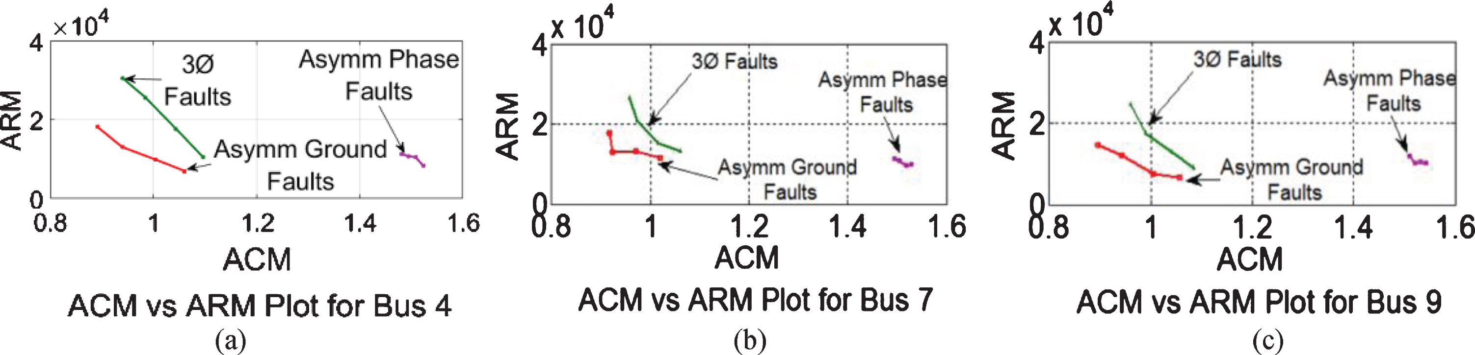
ACM vs ARM plots for 3Phase, Asymmetrical Ground and Asymmetrical Phase faults at (a) Bus 4, (b) Bus 7 and (c) Bus 9 obtained for IEEE-9 Bus system at 20%, 40%, 60% and 80% of the length of the transmission line.

5.2 IEEE-14 Bus system

The procedure and methodology to obtain the parameters for identification and location are kept the same for this case also. However, the number of cases considered here are more in number. It was observed that in the IEEE-14 bus system, the sparsity matrix of Bus 2 & 13 is significantly less, which indicates that the number of interconnections is more. Hence, such buses are considered for identifying and locating the type of faults. In total, seven cases have been simulated with 12 types of classes as defined in Table 1 totaling to 84 (12 classes x 7 fault zones) different cases. In the case of IEEE-9 Bus, the total number of cases is 36 (12 classes × 3 fault zones). The signal between t = 0.32 to 0.38 s has been considered for analysis with fault time from t = 0.32 to 0.36 s. The sampling time is set to 200μs. The values of the extracted parameters, ACM and ARM, are obtained and shown in Fig. 7. Similar to the previous case of IEEE-9 Bus, the area of ARM higher in comparison to ACM.

Fig. 7

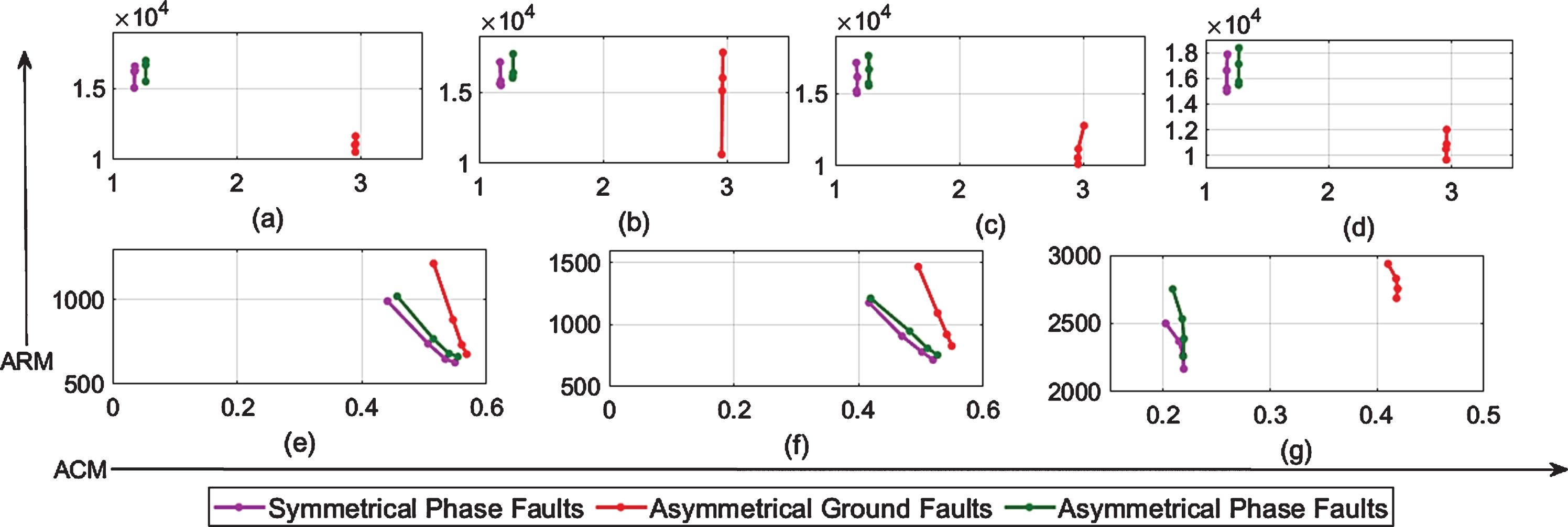
ACM vs ARM plots for 3-Phase, Asymmetrical Ground and Asymmetrical Phase faults between Bus 2&1, 2&3, 2&4, 2&5, 13&6, 13&12 and 13&14 at 20%, 40%, 60% and 80% of the length of transmission line.

The plot between ARM and ACM, as shown in Fig. 7 are for Symmetrical Phase fault, Asymmetrical Phase fault and Asymmetrical Ground faults in the IEEE-14 Bus power system. It is visible from the plot that all type of faults occurring between the buses 2-1, 2-3, 2-4, 2-5, 13-6, 13-12 and 13-14 have been successfully identified along with the location of the fault. It implies that if this algorithm is incorporated in the Power Quality Monitoring system, the exact location, along with the type of fault, can be visualized in <1 sec. It is a significant advantage of the proposed methodology, and such an approach is reported for the first time in the literature.

It was observed that the variation of ARM and ACM is more with the oscillations/impulses in the waveform, similar to the previous case of the IEEE-9 bus system. In this case of IEEE-14 Bus system, the variation in ARM and ACM due to the inception of fault during the time of voltage rise is also considered. It is very uncommon in a power system that the fault occurs at zero crossings only. Hence, faults occurring at non-zero crossings are also of significant concern, and the same has been considered for identification along with the location.

Figure 8 shows the Voltage waveform recorded at Bus 2 during an Asymmetrical Fault between Bus 2 and 3 at 20%, 40%, 60% and 80% of the length of the transmission line. It is observed that the oscillations are high for fault at 80% of the transmission line length from Bus-2, and the variation is similar for all types of faults. The ARM and ACM values are dynamic and vary with such oscillating magnitudes. Thus, the proposed methodology is sound in preserving the property of the input signal, thereby providing discriminative values for different faults at different locations. Further, the pattern is the same for the cases of faults occurring between various buses like Bus 2 & 4, Bus 13 & 12 and other considered cases.

Fig. 8

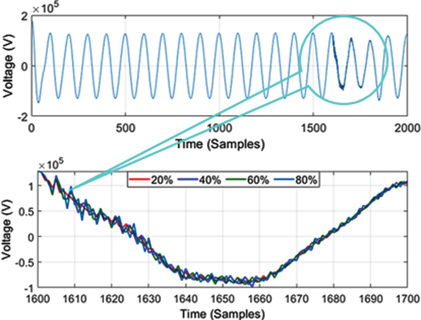
Voltage waveform during an Asymmetrical Ground Fault between Bus 2 and 3 at 20%, 40%, 60% and 80% of the length of transmission line for fault duration of t = 0.32 to 0.36 s with a sampling time of 0.2 ms (from 1600 to 1900 samples) and burst view for t = 0.3 s to 0.34 s.

Secondly, the values of ARM and ACM also varies with the time/angle of fault inception. Figure 9 shows the variation in voltage during the start of fault at t = 0.32 s. An impulsive voltage is seen at the beginning of the fault which is due to the reason that the fault has occurred during the rise of the sinusoidal voltage at an angle of 97.2°, i.e. away from zero crossing at t = 0.3146 s. However, no oscillations are seen in the rest of the signal as compared to Fig. 8. The ARM and ACM values of this particular case also vary similar to the previous case discussed above.

Fig. 9

Voltage waveform during an Asymmetrical Ground Fault between Bus 13 and 6 at 20%, 40%, 60% and 80% of the length of transmission line for fault duration of t = 0.32 to 0.36 s and burst view for t = 0.3 s to 0.34 s.

In the case of faults between Bus 13-12 and Bus 13-14, it was observed that the effect of angle/time of inception of fault is very less and there are no oscillatory intermediate transients due to the nearest power/generating station. Figure 10 indicates the absence of both the phenomenon which were present in the previous cases. The variation of ARM and ACM is like those which are mentioned in Table 2 of IEEE-9 Bus case. The reason is that being there is no dynamic variation in the magnitude and frequency during the occurrence of faults.

Fig. 10

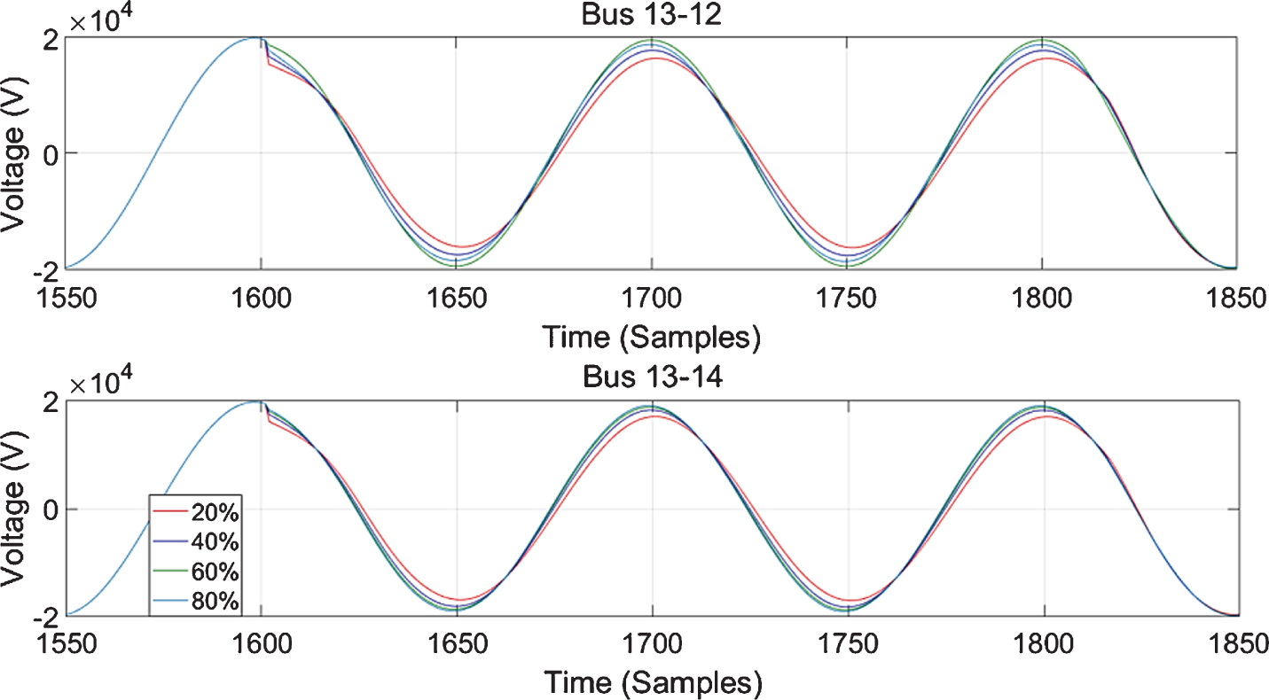
Voltage waveform during an Asymmetrical Fault between Bus 13&12, Bus 13&14 at 20%, 40%, 60% and 80% of the length of transmission line for fault duration of t = 0.32 to 0.36 s i.e. t = 1600 to 1800 samples.

Hence, it is visible that the proposed algorithm adapts to the type and nature of faults, i.e. the number of phases involved and also the transients involved in it. By revisiting Fig. 7, it can be mapped that first data point of all the three faults corresponds to faults at 20% of the length of the transmission line for the cases 2-1, 2-3, 2-4, 2-5, 13-6 whereas the first data point is 80% of the length of the transmission line for the case of faults at 13-12 and 13-14.

The values of ARM vary due to the presence of frequency components other than the fundamental frequency as in the case of impulsive and oscillatory transients. Whereas, the values of ACM vary with the increase or decrease in the magnitude of the input voltage waveform. The plot between these parameters provides a robust platform for dotting the type and location of faults. Since the type and location of faults have been discriminated, the extracted features are fed to the fuzzy system with the input MFs as shown in Fig. 4. Table 3 shows the rules defined in the fuzzy logic tool for identification of the type of fault. All the rules are defined as per the range of values obtained from the extracted features of ARM and ACM.

Table 3

FIS Rule Base designed for Identifying the Type of Fault

S. No.	Rules
1	If (ARM is R11) and (ACM is C2) then (TYPE-OF-FAULT is F1) (1)
2	If (ARM is R10) and (ACM is C2) then (TYPE-OF-FAULT is F2) (1)
3	If (ARM is R7) and (ACM is C5) then (TYPE-OF-FAULT is F3) (1)
4	If (ARM is R4) and (ACM is C5) then (TYPE-OF-FAULT is F4) (1)
5	If (ARM is R5) and (ACM is C6) then (TYPE-OF-FAULT is F5) (1)
6	If (ARM is R4) and (ACM is C6) then (TYPE-OF-FAULT is F6) (1)
7	If (ARM is R4) and (ACM is C7) then (TYPE-OF-FAULT is F7) (1)
8	If (ARM is R1) and (ACM is C7) then (TYPE-OF-FAULT is F8) (1)
9	If (ARM is R8) and (ACM is C1) then (TYPE-OF-FAULT is F9) (1)
10	If (ARM is R6) and (ACM is C2) then (TYPE-OF-FAULT is F10) (1)
11	If (ARM is R3) and (ACM is C4) then (TYPE-OF-FAULT is F11) (1)
12	If (ARM is R1) and (ACM is C6) then (TYPE-OF-FAULT is F12) (1)

It has already been explained that all the MFs of the fuzzy system are triangular as per the variation in the range of values. The output MFs are also considered as triangular in line with the input MFs. In the rule base, the names of various classed defined in Table 1 are used for identifying and locating different types of power system faults. The surface plot obtained for the set of rules is as shown in Fig. 11.

Fig. 11

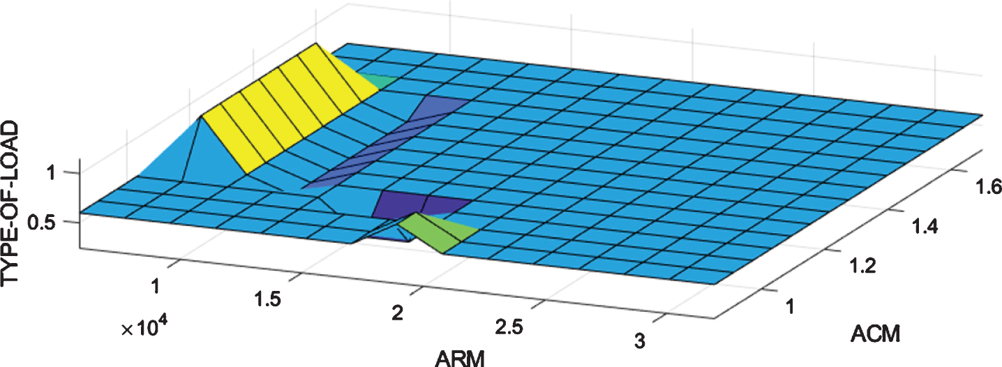
Surface plots for the fuzzy rules as defined in Table 4.

As mentioned earlier, 1/3rd of the data set obtained has been used to train the proposed fuzzy system. The other 1/3rd part has been used for validation and the output obtained is as desired. The remaining 1/3rd values (i.e. 36) have been used for testing. After successful testing, the model is simulated for 120 times for each of the considered 12 fault cases thus totaling to 1440 simulations..

Table 4 shows the results obtained along with the validation of results with SVM based machine learning technique, for the same datasets. The accuracy obtained for the SVM and the proposed methodology is 99.31% and 99.24% respectively. However, the time taken by the SVM based technique for training and testing is not consistent. It can be observed that the SVM algorithm has taken 7.61 seconds in one instance and 4.47 seconds in another, leading to variable identification time. Whereas, the proposed technique takes only 0.151 s in all instances, thus maintaining the consistency and making the proposed algorithm 39 times faster than SVM. This shows the efficacy of the proposed methodology of ST + Fuzzy logic.

Table 4

Values of Extracted Parameters Obtained from Simulations of Various Case Studies of IEEE-9 and IEEE-14 Bus system with comparison of results obtained by SVM

Variable Name	Count of correct identifications for 120 simulations		Time taken for identification in seconds		Accuracy (in %)
	Proposed ST + Fuzzy	ST + SVM	Proposed ST + Fuzzy	ST + SVM	Proposed ST + Fuzzy	ST + SVM
F1	119	119	0.151	4.47	99.17	99.17
F2	118	119	0.151	7.61	98.33	99.17
F3	119	119	0.151	7.89	99.17	99.17
F4	120	120	0.151	5.57	100.00	100.00
F5	120	120	0.151	6.61	100.00	100.00
F6	119	119	0.151	7.93	99.17	99.17
F7	118	118	0.151	4.58	98.33	98.33
F8	119	119	0.151	4.47	99.17	99.17
F9	119	119	0.151	5.68	99.17	99.17
F10	119	119	0.151	7.56	99.17	99.17
F11	120	120	0.151	6.35	100.00	100.00
F12	119	119	0.151	4.56	99.17	99.17
		Average=	0.151	6.107	99.24	99.31

Additional results are obtained by varying the sampling frequency from 2 kHz to 10 kHz. However, it was found that a higher sampling frequency is increasing the calculation burden and whereas a lower frequency is decreasing the accuracy. It was also found that there is a difference of 0.2 to 0.3 sec of ST algorithm computation time in the next higher sampling frequency, which is equal to 10 to 15 cycles of power system voltage. This increase in computation time can make the algorithm less fast, leading to slow remedial actions.

At a higher sampling frequency, the accuracy is getting saturated with an increasing value of 0.1 –0.3% for every 1 kHz. Further, a frequency of 5 kHz is the standard sampling frequency found in various measuring and monitoring equipment available in the market. Hence, the results obtained at 5 kHz sampling frequency are found to be more optimal, as shown in Fig. 12. The comparative results with the proposed methodology of ST + Fuzzy are shown in Table 5. It is visible that the proposed method has maintained high accuracy with the least time and features in a noisy environment.

Fig. 12

Variation in accuracy and computation time due to change in Sampling frequency.

Table 5

Comparison with the results reported in the literature in the last 5 years using various methods

Ref. No.	Method Used	Interconnected power system used (Yes/No)	Configuration of the system	Noise considered (Yes/No)	No. of Inputs/features extracted	Time for Identification (in sec)	Accuracy reported (%)	Research Gap
[17]	ANN	Yes	2 Bus 2 Grid system	No	6	Not Mentioned	100	Fastness and Noise level of algorithm not reported
[18]	Phasor Measurement Units	Yes	13 Bus 2 Generator	No	5		100
[19]	ANN	No	1 Generator, 52 Bus System	No	12		100
[20]	Petrinets	No	1 Grid, Radial System	No	12		Not Available
[21]	Wavelet &Fuzzy	Yes	IEEE-13 Bus &27 Bus	Yes	4		95	Fastness not mentioned
[22]	ANN with 35 Neurons	Yes	IEEE-14 Bus	No	6		100	Fastness and Noise level of algorithm not reported
[23]	SVM	Yes	2 Generator, &34 Nodes	No	9		99.19
This paper	Stockwell Transform &Fuzzy	Yes	IEEE-9 &IEE3-14 Bus	Yes	2	0.15	99.24	All research gaps addressed

6 Conclusions

A new methodology based on ST for identification and localization of different types of power system faults in standard IEEE-9 and IEEE-14 Bus power system has been presented. Three types of faults, i.e., Asymmetrical Phase, Asymmetrical Ground, and Symmetrical Faults occurring at 20% to 80% of the length of the transmission line, have been considered. The area under the envelope of various Gaussian windows of the Stockwell Transform matrix has been used at pre-parameter extraction, which is found to be effective with a lower computational burden. It is found that the proposed methodology identifies both oscillatory and impulsive transients present in a power system fault. Such information is useful for analyzing the after-effects of the power system faults.

Also, a Mamdani Fuzzy Decision Box is implemented to minimize misinterpretation and to improve the precision of the proposed technique. The Fuzzy decisions are found to be 99.24% accurate in determining and identifying the unknown types of power system failures that can occur dynamically in any location in a power system. Attempts have been made in the proposed approach to reduce the computational burden so that it can be realized into a low-cost real-time framework. Further, it can be used as a primary tool for developing an Integrated Power Quality Monitoring system.

References

Greenwood

, Electrical Transients in Power Systems, 2nd ed., New York: John Wiley & Sons, (1991).

Lobos

, Rezmer

and Koglin

H.J.

, Analysis of power system transients using wavelets and Prony method, Proceedings of IEEE Porto Power Tech Conference, (2001). DOI:10.1109/PTC.2001.964820

Janicek

, Mucha

and Ostrozlik

, A new protection relay based on fault transient analysis using wavelet transform, Journal of Electrical Engineering 58(5) (2007), 271–278. http://iris.elf.stuba.sk/cgibin/jeeec?act=abs&no=5_107&ttl=5.

Stockwell

R.G.

, Mansinha

and Lowe

L.P.

, Localization of the complex spectrum: The S transform, IEEE Trans on Signal Processing 44(4) (1996), 998–1001. DOI: 10.1109/78.492555

Stockwell

R.G.

, S-transform analysis of gravity wave activity from a small scale network of airglow imagers. PhD Thesis. https://ui.adsabs.harvard.edu/abs/1999PhDT........98S/abstract.

Pinnegar

C.R.

and Mansinha

, The S-transform with windows of arbitrary and varying shape, Society of explorations Geophysicists 68 (2003), 381–385. https://dx-doi-org.web.bisu.edu.cn/10.1190/1.1543223.

Ventosa

, Simon

, Schimmel

, Dañobeitia

J.J.

and Mànuel

, The S-transform from a wavelet point of view, IEEE Transactions on Signal Processing 44(7) (2008), 2771–2777. DOI: 10.1109/TSP.2008.917029

Dash

P.K.

, Panigrahi

B.K.

and Panda

, Power quality analysis using S–Transform, IEEE Transactions on Power Delivery 18(2) (2003), 406–411. DOI: 10.1109/MPER.2002.4312414

Lee

I.W.C.

and Dash

P.K.

, S-Transform-based intelligent system for classification of power quality disturbance signals, IEEE Transactions on Industrial Electronics 50(4) (2003), 800–805. DOI: 10.1109/TIE.2003.814991

10.

Zhao

and Yang

, Power quality disturbance recognition using S-Transform, IEEE Conference 6 (2006), 1–7. DOI: 10.1109/TPWRD.2006.881575

11.

Zhang

, Li

K.C.

and Hu

W.B.

, Automated classification of power quality disturbances using the S-Transform, Proc. of the 2008 Int. Conf. on Wavelet Analysis and Pattern Recognition (2008), 321–326. DOI:10.1109/ICWAPR.2008.4635797

12.

Schimmel

, Gallart

and Simon

, An alternative inverse S-Transform for filters with time-frequency localization, Proc. of the 4th International Symposium on Image and Signal Processing and Analysis (2005), 424–429. DOI:10.1109/ISPA.2005.195449

13.

Pei

S.C.

and Wang

P.W.

, Modified inverse S-Transform for filtering in time-frequency spectrum, ICASSP 7 (2007), 1169–1172. DOI: 10.1109/ICASSP.2007.367050

14.

Pei

S.C.

and Wang

P.W.

, New discrete inverse S-Transform with least square filtering, ICASSP 7 (2009), 2989–2992. DOI: 10.1109/ICASSP.2009.4960252

15.

Simon

, Ventosa

, Schimmel

, Heldring

, Danobeitia

J.J.

, Gallart

and Manuel

, The S-Transform and its inverses: side effects of discretizing and filtering, IEEE Transactions on Signal Processing 55(10) (2007), 4928–4937. DOI: 10.1109/TSP.2007.897893

16.

Srikanth

, Chandel

A.K.

and Naik

K.A.

, Identification of Power Quality Events Using Inverse Properties of S Transform, IEEE PES Power system conference & exposition, (2011), 20–23. Phoenix, Arizona, USA. DOI:10.1109/PSCE.2011.5772513

17.

Jamil

, Sharma

S.K.

and Singh

, Fault detection and classification in electrical power transmission system using artificial neural network, Open Access Research First Online: 09 July 2015. DOI:10.1186/s40064-015-1080-x

18.

Gopakumar

, Reddy

M.J.B.

and Mohanta

D.K.

, Fault Detection and Localization Methodology for Self-healing in Smart Power Grids Incorporating Phasor Measurement Units, Electric Power Components and Systems 43(6) (2015), 695–710. DOI: 10.1080/15325008.2014.995839

19.

Lala

, Karmakar

and Ganguly

, Fault Detection and Localization using Coninuous Wavelet Transform and Artificial Neural Network Based Approach in Distribution System, International Journal on Electrical Engineering and Informatics (2018), 203–219. DOI Number: 10.15676/ijeei.2018.10.2.1

20.

Sreerama

and Swarup

K.S.

, Detection, localization and fault diagnosis using Petri Nets for smart power distribution grids, 2017 7th International Conference on Power Systems (ICPS), Pune, (2017), 596–600. DOI:10.1109/ICPES.2017.8387363

21.

Jamil

, Singh

and Sharma

, Fault identification in electrical power distribution system using combined discrete wavelet transform and fuzzy logic, Journal of Electrical Systems and Information Technology 2 (2015), 257–267. https://doi.org/10.1016/J.JESIT.2015.03.015.

22.

Karić

, Konjic

and Jahić

, Power System Fault Detection, Classification and Location using Artificial Neural Networks, (2018).In: M. Hadžikadić, S. Avdaković, (eds) ATSA. IAT 2017. Lecture Notes in Networks and Systems, vol 28. Springer, Cham. https://doi.org/10.1007/978-3-319-71321-2_8.

23.

Perez

, Vásquez

and Viloria

, An intelligent strategy for faults location in distribution networks with distributed generation, J Intell Fuzzy Syst 36 (2019), 1627–1637. DOI: 10.3233/JIFS-18807

24.

MATLAB/SIMULINK 7.6.