An intuitionistic fuzzy neural network with gaussian membership function

Abstract

In this study, an intuitionistic fuzzy neural network (IFNN) with Gaussian membership function and Yager-generating function is proposed. Since intuitionistic fuzzy logic (IFL) considers membership, non-membership and hesitation values simultaneously, the incorporation of the concept of IFL into a fuzzy neural network (FNN) can enhance the performance of an FNN. A back-propagation learning algorithm is developed to optimize the IFNN parameters and weights. The proposed IFNN is applied to ten problems, including nonlinear control and prediction problems. The computational results indicate that the proposed IFNN is more efficient than conventional algorithms, such as artificial neural networks (ANN), fuzzy neural networks (FNN), and a support vector regression (SVR).

Keywords

Fuzzy neural network intuitionistic fuzzy sets fuzzy systems

1. Introduction

Fuzzy neural networks (FNNs), a popular research topic, have been successfully applied in many fields, including control, pattern recognition, classification, forecasting, and bioengineering [1 –11]. Basically, an ANN is a system derived from neurophysiology models, and functions by neural connections between many different processing elements, each analogous to a single neuron in a biological brain. Thus, ANN consists of a collection of simple, nonlinear computing elements, whose inputs and outputs are connected together to form a network [12]. However, a disadvantage of ANNs is that while a particular result may be obtained from the network, there is no explanation of how the network arrived at that result [13]. Fuzzy modeling [14], which is used to fuse decisions from different variables, requires an approach that learns from experience. For optimization, ANN learning algorithms are used to enhance the performance of fuzzy systems. Fuzzy IF-THEN rules are generated and adjusted, using the numerical data from these learning methods [15].

FNNs have the low-level learning and computational power of neural networks. In addition, fuzzy systems combine high-level, human thinking and reasoning ability, unlike artificial neural networks. The Takagi–Sugeno (TS) [16] method is a fuzzy control method developed in 1985. This method is widely used to control nonlinear systems, since the fuzzy control model can efficiently represent a nonlinear system, using a set of linear subsystems. Therefore, Lin and Lee [2] proposed the so-called neural-network-based fuzzy logic control system (NNFLCS). The low-level learning power of ANNs is used for fuzzy logic systems, and combines the normal connectionist architecture with a high-level meaning that is comprehensible. Furthermore, a different FNN, called an adaptive network-based fuzzy inference system (ANFIS) was proposed by Jang [17]. In ANFIS, there are five layers in the network architecture, and it employs a Sugeno fuzzy system. In order to train parameters, ANFIS uses a back-propagation algorithm to obtain membership functions. In addition, it determines the coefficients of the linear combinations in the consequences of the rule by a least mean squares algorithm [18]. Kuo and Cohen [19] employed the TS model for fuzzy inference to propose a feed-forward ANN.

The above FNNs are, however, only appropriate for numerical data. However, expert knowledge is qualitative, or cannot be quantified, so some studies have attempted to address this problem. Ishigami et al. [20] proposed learning methods for ANNs that utilize not only numerical data, but also expert knowledge, which is represented by fuzzy IF-THEN rules. Buckley and Hayashi [21] surveyed learning algorithms, and enhanced the training performance for FNNs, and Buckley proposed some techniques for error back-propagation learning algorithms. Unlike artificial neural networks, the advantage of FNNs is that the fuzzy inference rules can be explained by the IF-THEN rules. This allows the relationship between the input and output variables to be explained clearly. However, the fuzzy logic in FNNs considers only the degree of the membership function, and there still exists a degree of uncertainty.

However, according to the definition of intuitionistic fuzzy logic (IFL), the degree of uncertainty can be reduced. Sotirov and Atanassov [22] proposed feed forward neural networks (FFNNs) with IFL. Recently, IFL has also been applied to data mining [23]. Li et al. [24] proposed the max-min intuitionistic fuzzy Hopfield neural network (IFHNN), which can converge to a stable point within finite iterations under suitable extra conditions. Zhou et al. [25] proposed an IFNN model with a triangular membership and a two-step dynamic optimal training algorithm.

In light of the above, the purposes of this study are summarized as follows. In the proposed IFNN system, the Gaussian function is considered as the membership function, and the Yager-generated function is employed to obtain the membership value with the hesitation value. To optimize the connecting weights and parameters of the proposed IFNN, a back-propagation algorithm is developed to train the proposed IFNN system. Ten benchmark problems are applied to evaluate the performance of the proposed IFNN system, and the proposed IFNN is compared with FNN, ANN and SVR. Furthermore, in the computational results, the Wilcoxon signed-rank test is employed to verify the statistical significance.

The remainder of this paper is arranged as follows. Intuitionistic fuzzy sets are introduced in Section 2. A back-propagation learning algorithm that is used to train the proposed IFNN is described in Section 3. In Section 4, ten computational experiments, using benchmark functions, demonstrate the performance of the proposed IFNN. Finally, conclusions are offered in Section 5.

2. Intuitionistic fuzzy sets (IFSs)

The concept of intuitionistic fuzzy sets (IFS) was introduced by Atanassov [28, 29], and included an additional attribute parameter called non-membership [30]. Bustince and Burillo [31] then showed that vague sets (VS) are a kind of IFS. Generally, IFS are useful means to describe and deal with vague and uncertain data. They have received wide attention in recent years. Many studies have applied IFS to solve complex problems such as data mining [23], decision-making [32 –39], clustering problems [40, 41], forecasting problems [42], pattern recognition [43 –45] and medical problems [46, 47]. IFS were proposed as an extension of fuzzy sets. An IFS A in a fixed set E is an objective of the expression: $A = {〈 x, μ_{A} (x), υ_{A} (x) 〉 | x \in E},$ (1) where the functions, μ_A : E → [0, 1] and υ_A : E → [0, 1] respectively denote the degree of the membership and the degree of non-membership of the element, and x ∈ E. Furthermore, the degree of uncertainty must be considered for an IFS, A in E. The degree of hesitation for an element, x ∈ E in A is defined as: $π_{A} (X) = 1 - μ_{A} (X) - υ_{A} (X),$ (2) where π_A (x) is the degree of hesitation of x to A and 0 ⩽ π_A (x) ⩽1 for all x ∈ E.

According to [29, 30], in order to describe an IFS completely, a model should include the membership function, non-membership function, and degree of hesitation. A concept of IFS is to consider the non-membership function, thereby obtaining the degree of hesitation. In order to demonstrate the IFS completely, the Yager-generating function [31] is employed in this study, as the advantage of the Yager-generating function is that, in the functions for each value of α ∈ (0, ∞), a particular fuzzy complement can be well defined, which includes non-membership and degree of hesitation. Thus, the intuitionistic fuzzy complement with Yager-generating functions is shown as: $N (x) = (1 - x^{a})^{1 / a}, a > 0$ (3) where N (1) =0 and N (0) =1.

Therefore, using Atanassov’s intuitionistic fuzzy complement with Yager-generating functions, IFS become: $A = {〈 x, μ_{A} (x), (1 - μ_{A} (x)^{α})^{1 / a} 〉 | x \in E},$ (4) and the degree of hesitation is: $π_{A} (x) = 1 - μ_{A} (x) - (1 - μ_{A} (x)^{α})^{1 / α} .$ (5)

After the definition of the functions in IFS, the degree of hesitation and the membership degree are calculated using a linear combination of μ_A (x) and υ_A (x).

Since the membership function, non-membership function, and degree of hesitation are defined, the intuitionistic fuzzy neural network (IFNN) is developed with the concept of IFS. The model of the proposed IFNN and the learning algorithm are illustrated in the following section.

3. Intuitionistic fuzzy neural network (IFNN)

This section describes the architecture of the IFNN proposed in this study. The learning algorithm and the parameter determination are also described in this section.

3.1. Intuitionistic fuzzy neural network

The advantage of fuzzy neural networks is that they combine the advantages of fuzzy control and artificial neural networks. They can also obtain the fuzzy IF-THEN rules after training. As a fuzzy neural network, the fuzzy IF-THEN rule is employed in IFNNs. The kth rule, which is instantiated as: $\begin{matrix} Rule k : IF x_{1} is A_{1 k} and x_{2} \\ is A_{2 k} and x_{n} is A_{nk} THEN y_{k} is B_{k} \end{matrix}$ (6) where x₁, …, x_n are the input variables, n is the number of input variable, and y_k is the output variable, means that the values of forecasting. A_1k, …, A_nk are the linguistic terms of the pre-condition with the Gaussian membership function. The rule format of IFNNs is the same as that of neuro-fuzzy systems.

An integration function, f is associated with the fan-in of a unit, and serves to combine information, activation, or evidence from other nodes. This function provides the net input for this node: $\begin{matrix} net - input & = & f (u_{1}^{k}, u_{2}^{k}, \dots, u_{p}^{k}; w_{1}^{k}, w_{2}^{k}, \\ \dots, w_{p}^{k}), \end{matrix}$ (7) where the superscript shows the layer number.

A second action of each node is to output an activation value (C (f)) as a function of its net-input: $output = o_{i}^{k} = C (f) .$ (8)

Basically, the IFNN architecture is the same as that of ANFIS. Next, the detailed computation of each layer is shown as follows:

Layer 1. The nodes in the layer only obtain an input value to the layer 2. $f = u_{i}^{1} and C = f .$ (9)

The link weight of layer 1 ( $w_{i}^{1}$ ) is 1.

Layer 2. In the proposed IFNN, the Gaussian function is employed for the membership function as follows: $f = M_{xi}^{j} (m_{ij}, σ_{ij}) = exp {- \frac{(u_{i}^{2} - m_{ij})^{2}}{σ_{ij}^{2}}},$ (10) where m_ij is the center (mean) and σ_ij is the width (variance) of the Gaussian function of the jth term of the ith input linguistic variable x_i.

According to: $C = 1 - (1 - f^{α})^{1 / α},$ (11) the link weight of layer 2 ( $w_{ij}^{2}$ ) can be interpreted as m_ij.

Layer 3. Using the fuzzy intersection operator, AND, to translate the degree of accommodation into firing strength: $f = min (u_{1}^{3}, u_{2}^{3}, \dots, u_{p}^{3}) and act = f .$ (12)

The link weight of layer 3 ( $w_{i}^{3}$ ) is 1.

Layer 4. This structure uses the Mamdani inference model. According to this inference model, this layer drives the OR operation of fuzzy inference: $f = \sum_{i = 1}^{p} u_{i}^{4} and C = min (1, f) .$ (13)

The link weight of layer 4 ( $w_{i}^{4}$ ) is 1.

Layer 5. The final layer of the IFNN architecture, and the defuzzification process is: $f = \sum m_{ij}^{5} σ_{ij}^{5} u_{ij}^{5} and C = \frac{f}{\sum σ_{ij} u_{i}^{5}},$ (14) where $m_{ij}^{5}$ and $σ_{ij}^{5}$ are the mean and the variance of the membership functions, respectively. The link weight at layer five ( $w_{ij}^{5}$ ) is $m_{ij}^{5} σ_{ij}^{5}$ .

For the supervised learning algorithm, many studies have employed the back-propagation (BP) algorithm [48 –50]. Back-propagation is a method to obtain gradients while trying to minimize the loss function for a neural network. Thus, to train the parameters for the proposed IFNN, the stochastic version of gradient (BP) algorithm is used for this supervised learning, and to minimize the error function as the objective as follows: $E = \frac{1}{2} (y (t) - \hat{y} (t))^{2},$ (15) where y (t) is the desired output, and $\hat{y} (t)$ is the current output.

The process begins at the output nodes. A backward pass is used to compute ∂E/∂Y for all of the hidden nodes. Assuming that φ is the adjustable parameter in a node (e.g., the center of membership function), the general learning rule used is as follows: $φ (t + 1) = φ (t) + η (- \frac{\partial E}{\partial φ}),$ (16)

Layer 5. The center parameter is updated using: $m_{i} (t + 1) = m_{i} (t) + η [y (t) - \hat{y} (t)] \frac{σ_{i} u_{i}}{\sum σ_{i} u_{i}} .$ (17)

Therefore, the width parameter is updated using: $\begin{matrix} σ_{i} (t + 1) = σ_{i} (t) + η [y (t) - \hat{y} (t)] \\ \frac{m_{i} u_{i} (\sum σ_{i} u_{i}) - (\sum m_{i} σ_{i} u_{i}) u_{i}}{(\sum σ_{i} u_{i})^{2}} \end{matrix}$ (18)

Layer 4. Only the error signals ( $ɛ_{i}^{4}$ ’s) are computed and propagated. The error signal, $ɛ_{i}^{4}$ is derived as follows: $ɛ^{4} = [y (t) - \hat{y} (t)] \frac{m_{i} σ_{i} (\sum σ_{i} u_{i}) - (\sum m_{i} σ_{i} u_{i}) σ_{i}}{(\sum σ_{i} u_{i})^{2}}$ (19)

Layer 3. As with layer four, only the error signals are computed. According to (15), the error signal is derived as: $\begin{matrix} - ɛ_{i}^{3} = \frac{\partial E}{\partial f_{i}} = \frac{\partial E}{\partial c_{i}} \frac{\partial c_{i}}{\partial f_{i}} \frac{\partial E}{\partial (net - input)^{4}} \\ = \frac{\partial (net - input)^{4}}{\partial c_{i}} = - ɛ_{i}^{4} \frac{\partial f^{4}}{\partial u_{i}^{4}} = - ɛ_{i}^{4} . \end{matrix}$ (20)

Therefore, the error is $ɛ_{i}^{3} = ɛ_{i}^{4}$ . If there are multiple outputs, then the error signal becomes $ɛ_{i}^{3} = \sum_{k} ɛ_{k}^{4}$ , where the summation is performed over the consequences of a rule node, and the error in a rule node is the summation of the errors of its consequences.

Layer 2. By (20), the adaptive rule for m_ij is derived as follows:

The adaptive rule is: $\begin{matrix} m_{ij} (t + 1) \\ = m_{ij} (t) - η \frac{\partial E}{\partial c_{i}} \cdot {f^{α_{i} - 1} [(1 - f_{i}^{α_{i}})^{\frac{1}{α_{i}} - 1}]} \cdot \end{matrix}$ (21)

The adaptive rule for σ_ij becomes: $\begin{matrix} σ_{ij} (t + 1) \\ = σ_{ij} (t) - η \frac{\partial E}{\partial c_{i}} \cdot {2 f_{i} - f^{α_{i} - 1} [(1 - f_{i}^{α_{i}})^{\frac{1}{α_{i}} - 1}]} \cdot (22) \end{matrix}$ (22)

Therefore, the adaptive rule for α_i becomes $\begin{matrix} α_{i} (t + 1) = α_{i} (t) - η \cdot [- \frac{1}{α_{i}^{2}} \cdot ln (1 - f_{i}^{α_{i}}) \cdot \\ (1 - f_{i}^{α_{i}})^{\frac{1}{α_{i}}} - \frac{1}{α_{i}} \cdot f^{α} \cdot ln f (1 - f_{i}^{α_{i}})^{\frac{1}{α_{i}}}] . (23) \end{matrix}$ (23)

In order to evaluate the performance of the proposed model, the mean square error (MSE) and the mean absolute difference (MAD) were used to measure the forecasting accuracy. The estimated values more accurately represented the actual values than those of the MSE or the MAD. The MAD is one of the natural measures of average error magnitude, and is an unambiguous measure. The expressions for the MSE and the MAD are shown in Equations (24 and 25), respectively: $MSE = \frac{1}{n} \sum_{i = 1}^{n} (y_{i} - a_{i})$ (24) $MAD = \frac{1}{N} \sum_{i = 1}^{N} | y_{i} - a_{i} |$ (25) where a_i is the actual value, y_i is the forecast value and n is the total number of data.

In order to test the proposed IFNN, this study used Matlab to program the code. Three different benchmark functions were used to verify the proposed model. This study compared the proposed IFNN with other algorithms, including a FNN, an SVR and an ANN. In the study, K-fold cross-validation was employed to evaluate the model. For K-fold cross-validation, the original sample was randomly assigned into K subsamples. From the K subsamples, a single subsample was retained as the verification data. In the testing process, the remaining K - 1 sub-samples were used as training data. The cross-validation process was repeated K times, or folded, and each K sub-sample was used exactly once as the verification data. The results of these folds in K were then averaged to produce a single estimate. The advantage of this approach is that random sub-samples repeat, in that all observations are used for training and testing, and each observation is used to authenticate once. Ten-fold cross-validation is commonly used, so the value of K used was 10. The goal was to determine whether the IFNN is significantly better than other algorithms.

In IFNN, the learning rate (η) significantly affects the learning efficiency. However, there are five parameters in the IFNN. In order to reduce the number of simulations, and evaluate the parameter combinations, the Taguchi method [51] was employed. The Taguchi method uses orthogonal arrays, which identify the main effects without the interactions between the parameters. So, even with a large number of parameters, it evaluates the values of parameters efficiently, and identifies the parameters that have a greater impact on performance.

Five factors with three levels were used to design the parameters for the IFNN. The notation of the factors are as follows: the mean learning rate (η_m), the standard deviation learning rate (η_s), the Yager-parameter learning rate (α_a), the weight learning rate (η_w), and the momentum (ρ). An L₂₇ (3⁵) orthogonal array was used for the experiment. The orthogonal array generated had 27 types of combination. The test for each combination was performed ten times, over five hundred iterations, to allow the optimal training parameters to be determined. This goal of the experiment was to determine the lowest MSE, the criterion used for the objective. The MINITAB program was used to perform the Taguchi experiment.

This study set the MSE as the objective. The smaller the MSE, the better, so this experiment featured the-lower-the-better characteristics. The S/N ratio is the signal to noise ratio, which was used to evaluate the quality and stability of the Taguchi experimental design. In the Taguchi experiment, the mean value and the S/N ratio were consistent. A lower mean value indicates a higher S/N ratio, and a lower mean indicates a generated product of better quality.

4. Computational results

This section discusses the evaluation of the proposed IFNN with the Gaussian membership function. Using the proposed IFNN, Matlab was used to design a computer program that simulated different cases in order to demonstrate the feasibility of the proposed IFNN. Each test problem had its own characteristics and corresponding number of inputs. The training results were used to demonstrate the convergence of the test data, in order to determine the utility of the proposed IFNN.

4.1. The simulation cases

Case 1. Ackley function

In this dataset, the Ackley function is described by: $\begin{matrix} f_{1} = - 20 \times exp (- 0.2 \times \sqrt{\frac{1}{n}} \sum_{i = 1}^{n} x_{i}^{2}) \\ - exp (\frac{1}{n} \sum_{i = 1}^{n} cos (2 π \cdot x_{i})) + 20 + e . \end{matrix}$ (26)

In the dataset, there are two variables, and the domain of x_i is -2 ⩽ x_i ⩽ 2, i = 1, 2. The global minimum of the function is (x₁, x₂) = (0, 0), A (x₁, x₂) =0. There are 1000 patterns, generated in the domain (– 2, 2).

Case 2. Lim et al. [52] non-polynomial function

The Lim et al. [52] non-polynomial function is described by: $f_{z} = \frac{1}{6} [(30 + 5 x_{1} sin (5 x_{1})) (4 + exp (- 5 x_{2})) - 100]$ (27)

This function is an example of a non-polynomial model, which exhibits a shape similar to that of a multivariate polynomial. Lim et al. [52] compared predictions from this function with predictions. The function is evaluated on the square x_i ∈ [0, 1], for all i = 1, 2. There are 1000 patterns, generated in the domain (0, 1), and the function is illustrated in Fig. 1.

Fig. 1

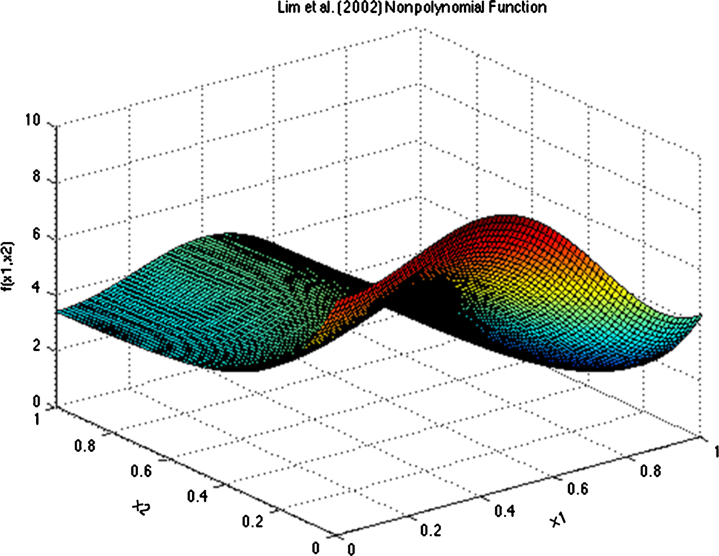
The Lim et al. non-polynomial function.

Case 3. Hartmann function

In this dat aset, the Hartmann function is described by: $f_{3} = - \sum_{i = 1}^{4} c_{i} exp [- \sum_{j = 1}^{n} a_{ij} (x_{j} - p_{ij})^{2}] .$ (28)

In the dataset, there are three variables, and the domain 0 ⩽ x_j ⩽ 1, j = 1, 2, 3. There are four local minima, and the global minimum is x^* = (0.114614, 0.555649, 0.852547), H_3,4 (x^*) -3.86278. There are 1000 patterns, generated in the domain (0, 1).

Case 4. Dette and Pepelyshev [53] exponential function

The Dette and Pepelyshev [53] exponential function is described by: $f_{4} = 100 (e^{- 2 / x_{1}^{1.75}} + e^{- 2 / x_{2}^{1.5}} + e^{- 2 / x_{3}^{1.25}})$ (29)

This function has asymptotes. It is used for the comparison of computer experiment designs. In addition to several hyperball domains, the function is evaluated on the cube x_i ∈ [0, 1], for all i = 1, 2, 3. There are 1000 patterns, generated in the domain (0, 1).

Case 5. Mackey-Glass time series [54]

The time-series prediction problem used is the chaotic Mackey–Glass time series, which is generated from the following differential equation: $f_{5} = \frac{dx (t)}{dt} = a \frac{x (t - τ)}{1 + x (t - τ)^{10}} - bx (t) .$ (30)

Following the majority of studies, the series has been generated using the next values for the parameters: a = 0.2, b = 0.1, and where τ ⩾ 17, the equation shows chaotic behavior. There are a total of 1000 patterns, generated from t = 124 to 1123.

Case 6. Gramacy and Lee [55] function

The Gramacy and Lee [55] function is described by: $f_{6} = exp [sin ((0.9 (x_{1} + 0.48))^{10})] + x_{2} x_{3} + x_{4}$ (31)

This function, used by Gramacy and Lee [55], is nonlinear in x₂ and x₃, and linear in x₄. In x₁, it begins to oscillate more quickly as it reaches the right bound of the interval [0, 1]. There is a random term ɛ ∼ N(0, 0.05²) added to the response. The function is evaluated on the hypercube x_i ∈ [0, 1], for all i = 1, …, 6. There are 1000 patterns, generated in the domain (0, 1).

Case 7. Friedman [56] function

The Friedman function is described by: $f_{7} = 10 (sin (π x_{1} x_{2}) + 20 (x_{3} - 0.5)^{2} + 10 x_{4} + 5 x_{5}$ (32)

The function is evaluated on the hypercube x_i ∈ [0, 1], for all i = 1, …, 5. There are 1000 patterns, generated in the domain (0, 1).

Case 8. Auto MPG6 prediction

This is a real world prediction problem of automobile city-cycle fuel consumption. The dataset contains 392 samples, and can be downloaded from KEEI [57]. There are five attributes including displacement, horsepower, weight, acceleration and model of year, while the output attribute is miles per gallon.

Case 9. Airfoil self-noise data [58]

This is a real world prediction problem of airfoil self-noise. In the datasets, there are 5 input attributes, and the attribute information is as follows:

Frequency, in Hertz;

Angle of attack, in degrees;

Chord length, in meters;

Free-stream velocity, in meters per second;

Suction side displacement thickness, in meters.

The only output is Scaled sound pressure level, in decibels. It contains 1503 instances, and can be download from the UCI machine learning repository [58].

Case 10. Yacht Hydrodynamics Data Set [58]

Prediction of residuary resistance of sailing yachts at the initial design stage is of great value for evaluating ships’ performance and for estimating their required propulsive power. Essential inputs include the basic hull dimensions and the boat velocity. The Delft data set consists of 308 full-scale experiments, which were performed at the Delft Ship Hydromechanics Laboratory for that purpose. The dataset can be downloaded from the UCI machine learning repository. The attribute information is as follows:

Longitudinal position of the center of buoyancy;

Prismatic coefficient;

Length-displacement ratio;

Beam-draught ratio;

Length-beam ratio;

Froude number.

The measured variable is the residuary resistance per unit weight of displacement, and residuary resistance per unit weight of displacement. The sources of benchmark datasets are summarized in Table 1. The datasets 1 to 7 are generated from the functions, and datasets 8 to 10 are real world problems.

Table 1

The benchmark datasets

Dataset	Source	Attributes
1	Ackley function	2
2	Lim et al. (2002) non-polynomial function	2
3	Hartmann function	3
4	Dette &Pepelyshev (2010) exponential function	3
5	Mackey-Glass time series	4
6	Gramacy &Lee (2009) function	4
7	Friedman (1991) function	5
8	Auto MPG6 prediction	5
9	Airfoil self-noise data	5
10	Yacht hydrodynamics data set	6

4.2. Comparison with other algorithms

This study used the Taguchi method [51] to determine the IFNN parameters. The results of the learning rate in ten cases are shown in Table 2. They demonstrate that the IFNN converges faster and gives more accurate results than the other three algorithms.

Table 2
The parameters of IFNN in ten cases.

η _m η _s η _a η _w ρ

Dataset 1. 0.005 0.005 0.009 0.05 0.01

Dataset 2. 0.005 0.001 0.001 0.05 0.01

Dataset 3. 0.0005 0.0005 0.001 0.01 0.05

Dataset 4. 0.001 0.001 0.005 0.05 0.01

Dataset 5. 0.0005 0.0005 0.001 0.05 0.01

Dataset 6. 0.0005 0.001 0.009 0.1 0.01

Dataset 7. 0.001 0.005 0.005 0.05 0.01

Dataset 8. 0.005 0.005 0.001 0.01 0.05

Dataset 9. 0.001 0.001 0.001 0.05 0.05

Dataset 10. 0.001 0.001 0.005 0.05 0.01

	η _m	η _s	η _a	η _w	ρ
Dataset 1.	0.005	0.005	0.009	0.05	0.01
Dataset 2.	0.005	0.001	0.001	0.05	0.01
Dataset 3.	0.0005	0.0005	0.001	0.01	0.05
Dataset 4.	0.001	0.001	0.005	0.05	0.01
Dataset 5.	0.0005	0.0005	0.001	0.05	0.01
Dataset 6.	0.0005	0.001	0.009	0.1	0.01
Dataset 7.	0.001	0.005	0.005	0.05	0.01
Dataset 8.	0.005	0.005	0.001	0.01	0.05
Dataset 9.	0.001	0.001	0.001	0.05	0.05
Dataset 10.	0.001	0.001	0.005	0.05	0.01

K-fold cross-validation (K = 10) was also used to confirm the statistical independence of the random process, and each experiment was implemented three times, for 500 iterations. Therefore, each experiment involved thirty runs. Table 3 shows the experimental results of training and testing MSE for each dataset, respectively. It shows that the IFNN had the smallest MSE value. Table 4 shows the MAD results for each algorithm. It shows that IFNN performs better than the other methods.

Table 3

Computational results (MSE) of training and testing data.

Training Data
		IFNN	FNN	ANN	SVR
Dataset 1.	mean	0.005050	0.005260	0.042325	0.005109
	STD.	0.000038	0.000063	0.000193	0.000000
	best	0.004963	0.005139	0.042000	0.005109
Dataset 2.	mean	0.000410	0.000307	0.002633	0.008128
	STD.	0.000015	0.000071	0.000137	0.000000
	best	0.000387	0.000146	0.002347	0.008128
Dataset 3.	mean	0.017032	0.020527	0.025788	0.048970
	STD.	0.005525	0.009288	0.000019	0.000000
	best	0.007588	0.003158	0.025745	0.048970
Dataset 4.	mean	0.001459	0.004118	0.000729	0.003369
	STD.	0.000528	0.000018	0.000003	0.000000
	best	0.000677	0.004081	0.000717	0.003369
Dataset 5.	mean	0.004753	0.008993	0.004398	0.006797
	STD.	0.001729	0.004075	0.000017	0.000000
	best	0.001953	0.000378	0.004372	0.006797
Dataset 6.	mean	0.013156	0.016594	0.018428	0.007058
	STD.	0.000969	0.001540	0.000595	0.000000
	best	0.012392	0.013471	0.016727	0.007058
Dataset 7.	mean	0.000012	0.023053	0.001716	0.004828
	STD.	0.000026	0.014151	0.000002	0.000000
	best	0.000004	0.003908	0.001713	0.004828
Dataset 8.	mean	0.004840	0.005049	0.007061	0.007058
	STD.	0.000019	0.000010	0.000011	0.000000
	best	0.004793	0.005026	0.007036	0.007058
Dataset 9.	mean	0.011695	0.030777	0.015668	0.015156
	STD.	0.001185	0.009304	0.000096	0.000001
	best	0.009029	0.021855	0.015388	0.015153
Dataset 10.	mean	0.001634	0.052973	0.002092	0.003836
	STD.	0.000150	0.003411	0.000395	0.000000
best		0.001391	0.043681	0.001201	0.003836
Testing Data
		IFNN	FNN	ANN	SVR
Dataset 1.	mean	0.005450	0.005714	0.043050	0.018309
	STD.	0.000116	0.000210	0.000190	0.000000
	best	0.005221	0.005281	0.042602	0.018309
Dataset 2.	mean	0.000518	0.000409	0.008395	0.000304
	STD.	0.000018	0.000074	0.000575	0.000000
	best	0.000477	0.000251	0.007492	0.000304
Dataset 3.	mean	0.019916	0.089320	0.030330	0.064308
	STD.	0.006849	0.018813	0.000040	0.000000
	best	0.005988	0.043652	0.030259	0.064308
Dataset 4.	mean	0.004136	0.005194	0.005487	0.000950
	STD.	0.001226	0.000025	0.000073	0.000000
	best	0.001324	0.005156	0.005346	0.000950
Dataset 5.	mean	0.005627	0.011616	0.004469	0.017716
	STD.	0.001946	0.006396	0.000025	0.000000
	best	0.001340	0.000918	0.004419	0.017716
Dataset 6.	mean	0.004563	0.018175	0.035277	0.017163
	STD.	0.004029	0.005102	0.001527	0.000000
	best	0.000350	0.012040	0.034770	0.017163
Dataset 7.	mean	0.000159	0.022197	0.002351	0.000178
	STD.	0.000116	0.018329	0.000013	0.000000
	best	0.000015	0.002100	0.002314	0.000178
Dataset 8.	mean	0.005439	0.007617	0.007336	0.007333
	STD.	0.000051	0.000070	0.000025	0.000000
	best	0.005298	0.007505	0.007290	0.007333
Dataset 9.	mean	0.021346	0.031787	0.014794	0.017120
	STD.	0.007013	0.009630	0.000169	0.000001
	best	0.008760	0.019733	0.014403	0.017118
Dataset 10.	mean	0.001885	0.058585	0.003091	0.008080
	STD.	0.000200	0.006128	0.000348	0.000000
	best	0.001517	0.047392	0.002532	0.008080

STD.: standard deviation.

Table 4

Computational results (MAD) of training data.

Training Data
		IFNN	FNN	ANN	SVR
Dataset 1.	mean	0.056001	0.054802	0.172499	0.156370
	STD.	0.000078	0.000795	0.000484	0.000000
	best	0.055884	0.052984	0.171663	0.156370
Dataset 2.	mean	0.004707	0.004412	0.030322	0.013193
	STD.	0.000709	0.000219	0.000416	0.000000
	best	0.003638	0.003877	0.029608	0.013193
Dataset 3.	mean	0.085036	0.102618	0.116048	0.160111
	STD.	0.045477	0.027009	0.000109	0.000000
	best	0.004462	0.051683	0.115783	0.160111
Dataset 4.	mean	0.001247	0.014295	0.020772	0.049340
	STD.	0.000248	0.002304	0.000072	0.000000
	best	0.000942	0.011618	0.020539	0.049340
Dataset 5.	mean	0.056802	0.064536	0.051335	0.080030
	STD.	0.013390	0.026926	0.000145	0.000000
	best	0.023730	0.026976	0.051053	0.080030
Dataset 6.	mean	0.061784	0.079891	0.088757	0.076445
	STD.	0.003594	0.006105	0.001991	0.000000
	best	0.056713	0.068838	0.083184	0.076445
Dataset 7.	mean	0.001959	0.085505	0.034425	0.062291
	STD.	0.000638	0.022808	0.000021	0.000000
	best	0.001247	0.046878	0.034393	0.062291
Dataset 8.	mean	0.017613	0.116033	0.054811	0.083641
	STD.	0.002638	0.056235	0.000041	0.000000
	best	0.009070	0.008178	0.054770	0.083641
Dataset 9.	mean	0.084433	0.137206	0.096193	0.056732
	STD.	0.004803	0.015147	0.000351	0.000000
	best	0.072777	0.116194	0.095121	0.056732
Dataset 10.	mean	0.025648	0.171057	0.016714	0.053312
	STD.	0.000937	0.008060	0.000601	0.000000
	best	0.024163	0.149200	0.015938	0.053312
Training Data
		IFNN	FNN	ANN	SVR
Dataset 1.	mean	0.057775	0.072152	0.174694	0.276160
	STD.	0.000166	0.001456	0.000515	0.000000
	best	0.057458	0.069468	0.173546	0.276160
Dataset 2.	mean	0.013070	0.026682	0.056428	0.087627
	STD.	0.002380	0.002566	0.002933	0.000000
	best	0.009447	0.018665	0.050714	0.087627
Dataset 3.	mean	0.094122	0.192674	0.124770	0.171074
	STD.	0.046242	0.024138	0.000181	0.000000
	best	0.005338	0.154557	0.124400	0.171074
Dataset 4.	mean	0.003287	0.016126	0.071456	0.015776
	STD.	0.001043	0.002450	0.000573	0.000000
	best	0.001764	0.011036	0.070349	0.015776
Dataset 5.	mean	0.063497	0.074139	0.060033	0.108020
	STD.	0.009910	0.028122	0.000694	0.000000
	best	0.044733	0.019574	0.058813	0.108020
Dataset 6.	mean	0.050151	0.085149	0.166902	0.058513
	STD.	0.023142	0.009423	0.001664	0.000000
	best	0.016887	0.067908	0.166250	0.058513
Dataset 7.	mean	0.007605	0.084775	0.045036	0.010650
	STD.	0.002635	0.027972	0.000141	0.000000
	best	0.002976	0.036696	0.044668	0.010650
Dataset 8.	mean	0.019301	0.122281	0.056860	0.174086
	STD.	0.003141	0.056583	0.000060	0.000000
	best	0.009969	0.007245	0.056795	0.174086
Dataset 9.	mean	0.115084	0.138990	0.094479	0.178533
	STD.	0.016467	0.017542	0.000629	0.000000
	best	0.074003	0.109901	0.093370	0.178533
Dataset 10.	mean	0.026390	0.181116	0.016121	0.074304
	STD.	0.001102	0.012704	0.000669	0.000000
	best	0.024322	0.152585	0.015278	0.074304

STD.: standard deviation.

Furthermore, ANOVA was employed to compare the efficiency of IFNN with other models, as shown in Tables 5 to 8. To verify the performance of the proposed IFNN, the non-parametric Wilcoxon signed-rank test [59] was employed. The test results are shown in Tables 9 and 10. The null hypothesis was rejected at p-values <0.05, which indicates a statistically significant difference between the IFNN and the other algorithms.

Table 5

The ANOVA of training data (MSE)

	sum sq	F	p-value
Dataset 1.	0.028	1072019.190	9.11E-192
Dataset 2.	0.025	1592.764	2.96E-69
Dataset 3.	0.239	1494458.221	4.83E-198
Dataset 4.	0.002	1979.344	2.92E-73
Dataset 5.	0.016	802.940	8.39E-57
Dataset 6.	0.000	296973.113	1.62E-167
Dataset 7.	0.066	14168.528	4.30E-110
Dataset 8.	0.085	61.935	1.88E-17
Dataset 9.	0.000	50.459	2.83E-15
Dataset 10.	0.014	116.509	2.48E-25

Table 6

The ANOVA of testing data (MSE)

	sum sq	F	p-value
Dataset 1.	0.022	662953.381	1.09E-182
Dataset 2.	0.115	636.098	1.18E-52
Dataset 3.	0.717	3665678.004	5.41E-215
Dataset 4.	0.024	721.216	6.95E-55
Dataset 5.	0.032	1034.017	2.31E-61
Dataset 6.	0.000	32993.046	4.99E-126
Dataset 7.	0.391	59431.945	3.90E-137
Dataset 8.	0.090	63.168	1.13E-17
Dataset 9.	0.003	1279.633	3.05E-65
Dataset 10.	0.043	653.143	4.01E-53

Table 7

The ANOVA of training data (MAD)

	sum sq	F	p-value
Dataset 1.	0.000	9317.126	3.33E-102
Dataset 2.	0.011	68745.516	6.95E-140
Dataset 3.	0.022	26448.936	7.39E-122
Dataset 4.	0.001	81486.439	4.29E-143
Dataset 5.	0.002	2253.108	1.17E-75
Dataset 6.	0.000	16923511.499	6.84E-244
Dataset 7.	0.035	396621.837	5.53E-173
Dataset 8.	0.011	971.911	3.06E-60
Dataset 9.	0.000	775164.679	1.22E-185
Dataset 10.	0.055	201515.862	3.41E-160

Table 8

The ANOVA of testing data (MAD)

	sum sq	F	p-value
Dataset 1.	0.001	32962.838	5.19E-126
Dataset 2.	0.057	3526.569	5.41E-84
Dataset 3.	0.058	52193.867	1.10E-134
Dataset 4.	0.001	1937.006	7.32E-73
Dataset 5.	0.014	1155.423	2.22E-63
Dataset 6.	0.001	31714.182	2.78E-125
Dataset 7.	0.077	25774.509	2.27E-121
Dataset 8.	0.254	709.120	1.39E-54
Dataset 9.	0.000	10492.290	1.94E-104
Dataset 10.	0.026	5586.675	1.34E-92

Table 9

The p-values of Wilcoxon signed-rank test (MSE)

Dataset	IFNN	FNN	ANN	SVR
1	–	0.000	0.000	0.000
2	–	0.000	0.000	1.000
3	–	0.000	0.000	0.000
4	–	0.000	0.000	1.000
5	–	0.000	1.000	0.000
6	–	0.000	0.000	0.000
7	–	0.000	0.000	0.102
8	–	0.000	0.000	0.000
9	–	0.000	1.000	1.000
10	–	0.000	0.000	0.000

Table 10

The p-values of Wilcoxon signed-rank test (MAD)

Dataset	IFNN	FNN	ANN	SVR
1	–	0.000	0.000	0.000
2	–	0.000	0.000	0.000
3	–	0.000	0.000	0.000
4	–	0.000	0.000	0.000
5	–	0.035	0.120	0.000
6	–	0.000	0.000	0.033
7	–	0.000	0.000	0.000
8	–	0.000	0.000	0.000
9	–	0.000	1.000	0.000
10	–	0.000	1.000	0.000

The MSE for training data indicates that IFNN can obtain better results than other compared algorithms. According to the results of the Wilcoxon signed-rank test, the proposed IFNN exhibited superior performance. This can attribute to several factors. Firstly, the back-propagation learning algorithm is able to train the network efficiently. Secondly, since the IFNN incorporates the concept of IFL, the degree of hesitation considers the membership degree and non-membership degree simultaneously. This can better define the degree of uncertainty. Due to the reduction of the uncertainty degree, the performance can be enhanced.

5. Conclusions

This study proposed an IFNN with Gaussian membership function, since previous studies have indicated that using the Gaussian function as the membership function can result in better performance for developing the FNN model [2 , 61]. In addition, the IFNN incorporates the concept of IFL. Thus, the degree of hesitation can consider the membership degree and non-membership degree simultaneously. The Yager-generated function was employed to obtain the membership degree with degree of hesitation. This study also developed a back-propagation learning algorithm to train the parameters and weights of the IFNN. Using ten benchmark problems to verify the proposed IFNN, the computational results indicate that the proposed IFNN outperforms the other three compared methods.

A possible direction for future is to employ metaheuristics, such as genetic algorithm and particle swarm optimization, to optimize the IFNN. In addition, the concept of multi-fuzzy set is a generalization of the concepts of both fuzzy set and intuitionistic fuzzy set [62]. Thus, a multi-fuzzy neural network can be considered for future work. Furthermore, applying the proposed method to solve real world forecasting problems will also be implemented.

References

L. A.

Zadeh , The concept of a linguistic variable and its application to approximate reasoning—I, Information sciences, 8 (1975), 199-249.

C.-T.

Lin and

C.S.G.

Lee , Neural-network-based fuzzy logic control and decision system, Computers, IEEE Transactions on 40 (1991), 1320-1336.

C.-F.

Juang and

C.-T.

Lin , An online self-constructing neural fuzzy inference network and its applications, Fuzzy Systems, IEEE Transactions on 6 (1998), 12–32.

R.-J.

Wai and

P.-C.

Chen , Intelligent tracking control for robot manipulator including actuator dynamics via TSK-type fuzzy neural network, Fuzzy Systems, IEEE Transactions on 12 (20004), 552–560.

C.-F.

Juang and

Lo , Zero-order TSK-type fuzzy system learning using a two-phase swarm intelligence algorithm, Fuzzy Sets and Systems 159 (2008), 2910–2926.

Hadavandi ,

Shavandi and

Ghanbari , Integration of genetic fuzzy systems and artificial neural networks for stock price forecasting, Knowledge-Based Systems 23 (2010), 800–808.

R.J.

Kuo ,

C.H.

Chen and

Y.C.

Hwang , An intelligent stock trading decision support system through integration of genetic algorithm based fuzzy neural network and artificial neural network, Fuzzy Sets and Systems 118 (2001), 21–45.

R.J.

Kuo ,

Wu and

C.P.

Wang , An intelligent sales forecasting system through integration of artificial neural networks and fuzzy neural networks with fuzzy weight elimination, Neural Networks 15 (2002), 909–925.

R.J.

Kuo ,

S.Y.

Hung and

W.C.

Cheng , Application of an optimization artificial immune network and particle swarm optimization-based fuzzy neural network to an RFID-based positioning system, Information Sciences 262 (2014), 78–98.

10.

J.M.

Andújar and

J.M.

Bravo , Multivariable fuzzy control applied to the physical-chemical treatment facility of a Cellulose factory, Fuzzy Sets and Systems 150 (2005), 475–492.

11.

R.J.

Kuo ,

S.M.

Hong ,

Lin and

Y.C.

Huang , Continuous genetic algorithm-based fuzzy neural network for learning fuzzy IF–THEN rules, Neurocomputing 71 (2008), 2893–2907.

12.

Rumelhart ,

Hinton and

Williams , Learning internal representations by error propagation, Parallel Distributed Processing: Explorations in the Microstructure of Cognition, Foundations, MIT Press, Cambridge, MA, 1986, pp. 318–362.

13.

Mitra and

Hayashi , Neuro-fuzzy rule generation: Survey in soft computing framework, Neural Networks, IEEE Transactions on 11 (2000), 748–768.

14.

L.A.

Zadeh , Fuzzy sets, Information and Control 8 (1965), 338–353.

15.

Shibata ,

Fukuda ,

Kosuge ,

Arai ,

Tokita and

Mitsuoka , Skill based control by using fuzzy neural network for hierarchical intelligent control, in Neural Networks, 1992. IJCNN., International Joint Conference on, 1992, pp. 81–86.

16.

Takagi and

Sugeno , Fuzzy identification of systems and its applications to modeling and control, Systems, Man and Cybernetics, IEEE Transactions on (1985), 116–132.

17.

J.-S.

Jang , ANFIS: Adaptive-network-based fuzzy inference system, Systems, Man and Cybernetics, IEEE Transactions on 23 (1993), 665–685.

18.

M.A.

Shoorehdeli ,

Teshnehlab and

A.K.

Sedigh , Identification using ANFIS with intelligent hybrid stable learning algorithm approaches, Neural Computing and Applications 18 (2009), 157–174.

19.

R.J.

Kuo and

P.H.

Cohen , Manufacturing process control through integration of neural networks and fuzzy model, Fuzzy Sets and Systems 98 (1998), 15–31.

20.

Ishigami ,

Fukuda ,

Shibata and

Arai , Structure optimization of fuzzy neural network by genetic algorithm, Fuzzy Sets and Systems 71 (1995), 257–264.

21.

J.J.

Buckley and

Hayashi , Can fuzzy neural nets approximate continuous fuzzy functions? Fuzzy Sets and Systems 61(1994), 43–51.

22.

Sotirov and

Atanassov , Intuitionistic fuzzy feed forward neural network, Cybernetics and Information Technologies 9 (2009), 71–76.

23.

Atanassov , Intuitionistic fuzzy logics as tools for evaluation of Data Mining processes, Knowledge-Based Systems 80 (2015), 122–130.

24.

Li ,

Yang and

Wu , Intuitionistic fuzzy hopfield neural network and its stability, Neural Network World 21 (2011), 461.

25.

Zhou ,

Zhao and

Zhang , An Intuitionistic Fuzzy Neural Network with Triangular Membership Function, in Proceedings of 2013 Chinese Intelligent Automation Conference vol. 254,

Sun and

Deng , Eds., ed: Springer Berlin Heidelberg, 2013, pp. 813–820.

26.

L.A.

Zadeh , Similarity relations and fuzzy orderings, Information Sciences 3 (1971), 177–200.

27.

L.A.

Zadeh , Is there a need for fuzzy logic? Information Sciences 178 (2008), 2751–2779.

28.

Atanassov and

Gargov , Interval valued intuitionistic fuzzy sets, Fuzzy Sets and Systems 31 (1989), 343–349.

29.

K.T.

Atanassov , More on intuitionistic fuzzy sets, Fuzzy Sets and Systems 33 (1989), 37–45.

30.

K.T.

Atanassov , Intuitionistic fuzzy sets: Springer, 1999.

31.

Burillo and

Bustince , Entropy on intuitionistic fuzzy sets and on interval-valued fuzzy sets, Fuzzy Sets and Systems 78 (1996), 305–316.

32.

Atanassov ,

Pasi and

Yager , Intuitionistic fuzzy interpretations of multi-criteria multi-person and multi-measurement tool decision making, International Journal of Systems Science 36 (2005), 859–868.

33.

H.-W.

Liu and

G.-J.

Wang , Multi-criteria decision-making methods based on intuitionistic fuzzy sets, European Journal of Operational Research 179 (2007), 220–233.

34.

Ye , Multicriteria fuzzy decision-making method using entropy weights-based correlation coefficients of interval-valued intuitionistic fuzzy sets, Applied Mathematical Modelling 34 (2010), 3864–3870.

35.

Beliakov ,

Bustince ,

Goswami ,

Mukherjee and

N.R.

Pal , On averaging operators for Atanassov’s intuitionistic fuzzy sets, Information Sciences 181 (2011), 1116–1124.

36.

T.-Y.

Chen , A comparative analysis of score functions for multiple criteria decision making in intuitionistic fuzzy settings, Information Sciences 181 (2011), 3652–3676.

37.

Chen and

Yang , A new multiple attribute group decision making method in intuitionistic fuzzy setting, Applied Mathematical Modelling 35 (2011), 4424–4437.

38.

Guo and

Li , An attitudinal-based method for constructing intuitionistic fuzzy information in hybrid MADM under uncertainty, Information Sciences 208 (2012), 28–38.

39.

Akram ,

Ashraf and

Sarwar , Novel applications of intuitionistic fuzzy digraphs in decision support systems, Scientific World Journal 2014 (2014).

40.

K.P.

Lin , A novel evolutionary kernel intuitionistic fuzzy C-means clustering algorithm, Fuzzy Systems, IEEE Transactions on (2013), 1–1.

41.

Akram and

W.A.

Dudek , Intuitionistic fuzzy hypergraphs with applications, Information Sciences 218 (2013), 182–193.

42.

K.-C.

Hung and

K.-P.

Lin , Long-term business cycle forecasting through a potential intuitionistic fuzzy least-squares support vector regression approach, Information Sciences 224 (2013), 37–48.

43.

Chaira and

Ray , A new measure using intuitionistic fuzzy set theory and its application to edge detection, Applied Soft Computing 8 (2008), 919–927.

44.

Dengfeng and

Chuntian , New similarity measures of intuitionistic fuzzy sets and application to pattern recognitions, Pattern Recognition Letters 23 (2002), 221–225.

45.

C.-M.

Hwang ,

M.-S.

Yang ,

W.-L.

Hung and

M.-G.

Lee , A similarity measure of intuitionistic fuzzy sets based on the Sugeno integral with its application to pattern recognition, Information Sciences 189 (2012), 93–109.

46.

Chaira , A novel intuitionistic fuzzy C means clustering algorithm and its application to medical images, Applied Soft Computing 11 (2011), 1711–1717.

47.

Kharal , Homeopathic drug selection using intuitionistic fuzzy sets, Homeopathy 98 (2009), 35–39.

48.

Liu ,

Wang ,

Golnaraghi and

Kubica , A neural fuzzy framework for system mapping applications, Knowledge-Based Systems 23 (2010), 572–579.

49.

Y.-H.

Chien ,

W.-Y.

Wang ,

Y.-G.

Leu and

T.-T.

Lee , Robust adaptive controller design for a class of uncertain nonlinear systems using online T–S fuzzy-neural modeling approach, Systems, Man, and Cybernetics, Part B: Cybernetics, IEEE Transactions on 41 (2011), 542–552.

50.

S.-B.

Roh ,

S.-K.

Oh and

Pedrycz , A fuzzy ensemble of parallel polynomial neural networks with information granules formed by fuzzy clustering, Knowledge-Based Systems 23 (2010), 202–219.

51.

Taguchi ,

Chowdhury and

Wu , Taguchi’s quality engineering handbook: Wiley, 2005.

52.

Y.B.

Lim ,

Sacks ,

Studden and

W.J.

Welch , Design and analysis of computer experiments when the output is highly correlated over the input space, Canadian Journal of Statistics 30 (2002), 109–126.

53.

Dette and

Pepelyshev , Generalized Latin hypercube design for computer experiments, Technometrics 52 (2010).

54.

M.C.

Mackey and

Glass , Oscillation and chaos in physiological control systems, Science 197 (1977), 287–289.

55.

R.B.

Gramacy and

H.K.

Lee , Adaptive design and analysis of supercomputer experiments, Technometrics 51 (2009), 130–145.

56.

J.H.

Friedman , Multivariate adaptive regression splines, The Annals of Statistics (1991), 1–67.

57.

Alcalá ,

Fernández ,

Luengo ,

Derrac ,

García ,

Sánchez , et al., Keel data-mining software tool: Data set repository, integration of algorithms and experimental analysis framework, Journal of Multiple-Valued Logic and Soft Computing 17 (2010), 255–287.

58.

Lichman , UCI machine learning repository (http://archive.ics.uci.edu/ml). University of California, School of Information and Computer Science, Irvine, CA, 2013.

59.

Demšar , Statistical comparisons of classifiers over multiple data sets, The Journal of Machine Learning Research 7 (2006), 1–30.

60.

Toprak and

İ.

Güler , Impulse noise reduction in medical images with the use of switch mode fuzzy adaptive median filter, Digital Signal Processing 17 (2007), 711–723.

61.

R.-J.

Kuo ,

M.-H.

Huang ,

W.-C.

Cheng ,

C.-C.

Lin and

Y.-H.

Wu , Application of a two-stage fuzzy neural network to a prostate cancer prognosis system, Artificial Intelligence in Medicine 63 (2015), 119–133.

62.

Sebastian and

T.V.

Ramakrishnan , Multi-fuzzy sets: An extension of fuzzy sets, Fuzzy Information and Engineering, Springer 1 (2011), 35–43.