The impact of subway operation on urban traffic: A GRA-BNs based study

Abstract

With the development of urbanization, urban traffic has exposed many problems. To study the subway’s influence on urban traffic, this paper collects data on traffic indicators in Nanchang from 2008 to 2018. The research is carried out from three aspects: traffic accessibility, green traffic, and traffic security. First, Grey Relational Analysis is used to select 18 traffic indicators correlated with the subway from 22 traffic indicators. Second, the data is discretized and learned based on Bayesian Networks to construct the structural network of the subway’s influence. Third, to verify the reliability of using GRA and the effectiveness of Bayesian Networks (GRA-BNs), Bayesian Networks with full indicators analysis and other four algorithms (Naive Bayes, Random Decision Forest, Logistic and regression) are employed for comparison. Moreover, the receiver operating characteristic (ROC) area, true positive (TP) rate, false positive (FP) rate, precision, recall, F-measure, and accuracy are utilized for comparing each situation. The result shows that GRA-BNs is the most effective model to study the impact of the subway’s operation on urban traffic. Then, the dependence relations between the subway and each index are analyzed by the conditional probability tables (CPTs). Finally, according to the analysis, some suggestions are put forward.

Keywords

Subway traffic accessibility green traffic traffic security Bayesian networks

1 Introduction

1.1 Background

The acceleration of China’s urbanization has led to rapid social and economic development. However, a series of urban problems, such as explosive population growth, population mobility, and the imbalance between supporting facilities and urban expansion, have emerged one after another, which has led to many traffic problems, resulting in limiting the healthy development of cities. The smooth flow of urban traffic not only reflects the level of urban management planning but also demonstrates the potential of the city’s future development. Table 1 reflects the top ten cities in the peak commuter congestion index in 2019. Unreasonable ground transportation planning and high car ownership are all causes of traffic congestion. This phenomenon has brought many urban development problems, such as transportation network safety, environmental noise pollution, electromagnetic interference, and other issues.

Table 1
National Traffic Congestion Ranking of 100 Cities in 2019

Rank City Peak commute congestion index Actual peak of commuting speed (km/h)

1 Chongqing 2.165 23.64

2 Beijing 2.040 25.12

3 Guiyang 1.979 25.76

4 Harbin 1.905 23.08

5 Changchun 1.777 26.69

6 Guangzhou 1.744 29.89

7 Shanghai 1.739 25.56

8 Xi’an 1.730 28.13

9 Hohhot 1.725 28.83

10 Wuhan 1.719 27.08

Rank	City	Peak commute congestion index	Actual peak of commuting speed (km/h)
1	Chongqing	2.165	23.64
2	Beijing	2.040	25.12
3	Guiyang	1.979	25.76
4	Harbin	1.905	23.08
5	Changchun	1.777	26.69
6	Guangzhou	1.744	29.89
7	Shanghai	1.739	25.56
8	Xi’an	1.730	28.13
9	Hohhot	1.725	28.83
10	Wuhan	1.719	27.08

To solve traffic problems in medium and large cities, urban road traffic in many cities has been optimized, and methods such as vehicle number travel, building BRT, widening roads, improving road traffic networks, and rush hours are used to relieve road traffic pressure. During the development of China’s rail transit, the growth rate of operating mileage is relatively high. From 2012 to 2019, the annual growth of rail transit operating mileage has exceeded 10%. The changes in operating mileage of China’s rail transit are shown in Fig. 1.

Fig. 1

Total length and growth rate of urban rail transit lines in China from 2012 to 2019.

As an urban infrastructure, the development of the subway is still developing rapidly throughout the country. The urban subway in mainland China completed 23.71 billion passenger trips throughout the year, increasing 2.64 billion people over the last year. The high efficiency, punctuality, environmental protection, and increased accessibility have been favored by all sectors of society and have gradually become the mainstay of public transportation in medium and large cities.

1.2 The impact of subway opening on the city

In recent years, many scholars have studied extensively when analyzing the impact of subway opening on cities. To study the accessibility of subway opening to urban traffic, Paloma Cáceres et al. [15] improved the accessibility in the public transport system by using available information (open data, semantic-aware knowledge) provided by transport organization; Wang [24] analyzed the relationship between community attributes and the subway home-price capitalization effect, asking whether the magnitude of the subway proximity premium is affected by neighborhood economic status and location; Trojanek and Gluszak [17] analyzed both spatial and time effects of subway availability on apartment prices in Warsaw; Seo and Nam [22] used the conventional hedonic price model and the spatial autoregressive combined model to examine the effect of subway accessibility on apartment prices for the three types of apartments. Furthermore, to illustrate the influence of subway construction on the evolution of urban spatial morphology, Miao et al. [27] used the concept of response displacement method to investigate the seismic characteristics of subway tunnel under spatially varying earthquake ground motions (SVEGMs). The research concluded that the development of rail transit strengthened Zhengzhou’s spatial development axis and affected the urban land use Structure optimization and gradually formed a multi-center urban spatial development structure; Li et al. [18] used a variety of remote sensing images, landscape metrics and gradient analysis to study the spatiotemporal dynamics of urban expansion and regional structure changes along the Guangzhou-Foshan intercity metropolis in the Pearl River Delta.

Moreover, the traffic evaluation system has always been a hot research topic for scholars in traffic evaluation, and there has not found a widely recognized traffic evaluation model. The reason is that traffic is often closely related to research on economy, environmental protection, and technology. Therefore, when a traffic evaluation model is being constructed, it tends to have a specific directionality. Ziedan [1] used multilevel negative binomial regression models to analyze light rail and streetcar collisions and injuries; Lin et al. [5] established a road network model in VISSIM to compare four different traffic organization plans. According to the different means of transportation, the existing research fields can be divided into public transportation, road transportation, rail transportation, etc. When studying the urban traffic evaluation system, scholars pay more attention to private cars’ impact on traffic. During the research process, indicators such as road traffic and car ownership often become essential aspects, while public transportation accounts for fewer influencing factors; research is more focused on traffic prediction. Gabriel Gomes [6] developed the Traffic Prediction System (TPS) model to generate the system’s real-time daily status prediction and large-scale distribution activities. Barros [4] studied the traffic conditions in residential areas and constructed an evaluation model using noise, pollution, and congestion as comprehensive evaluation indicators. Mark Wardman et al. [21] analyzed the urban traffic evaluation system and took noise and air quality as critical factors.

After detailed exploring the research on the application of the Bayesian networks and the urban traffic evaluation system, it is found that the Bayesian networks is widely used in traffic accidents, and it is mostly causal reasoning in traditional research. The research involves selecting the result as a class variable and the reason as an attribute variable. Scholars are confined to a particular aspect in studying the impact of subway opening on urban traffic but have not established a comprehensive evaluation system. Thus, this paper comprehensively analyzes the various traffic data of Nanchang subway since its official opening in December 2015 and the data before the opening of the subway from 2008 to 2015. It is constructed a comprehensive evaluation system from three aspects of traffic accessibility, green transportation, and safety for study to analyze the impact of subway opening on urban traffic. In addition, the paper also proposes a research method based on grey relational analysis and Bayesian networks method (GRA-BNs) learning to identify and screen the indicators with a high degree of relevance to subway opening and analyze the dependence between various indicators. The framework and technical route for this paper is shown in Fig. 2.

Fig. 2

Framework and technical route of this paper.

2 Methodology

2.1 Grey relational analysis

Grey Relational Analysis (GRA) refers to a quantitative expression of changes in the causal state in the development and evolution of various factors and results of a system. It is a method of comparing the intimacy between multiple factors and results. The fundamental core is to adopt and determine the degree of similarity between the reference data column’s geometric state and several data columns to determine the distance relationship, which expresses the degree of correlation of the curve [11].

The first step of utilizing the GRA is to determine a series of data as an evaluation index, i.e., the reference series determines the statistical data series of the fixed characteristics in the system, and the comparison series represents the data series that affect the behavior of the system. The reference series is as follows: $Y^{'} = [Y_{1}^{'}, Y_{2}^{'}, . . ., Y_{3}^{'}]^{T}$ (1)

The comparison series is as follows: $(X_{1}^{'}, X_{2}^{'}, . . ., X_{n}^{'}) = [\begin{matrix} X_{11}^{'} X_{21}^{'} . . . X_{n 1}^{'} \\ X_{12}^{'} X_{22}^{'} . . . X_{n 2}^{'} \\ . . . . . . . . . . . . \\ X_{1 m}^{'} X_{2 m}^{'} . . . X_{nm}^{'} \end{matrix}]$ (2) where m is the number of indicators, $X_{i}^{'} = {[X_{i 1}^{'} X_{i 1}^{'} . . . X_{im}^{'}]}^{T}, i = 1, 2, . . ., n$ .

Due to the differences in definitions, meanings, units, and value ranges of the indicators, the dimensions of the indicators are inconsistent, making it inconvenient for direct comparison. Therefore, when GRA is adopted for data, it is usually necessary to pre-process the data without dimension, and finally compare and analyze each index. $X_{ik} = \frac{X_{ik}^{'}}{\frac{1}{m} \sum_{k = 1}^{m} X_{ik}^{'}} (i = 1, 2, . . ., n; k = 1, 2, . . ., m)$ (3)

The grey relativity generally refers to the difference trend of geometric states between the curves, and the difference is the size of the correlation level. The calculation formula of each correlation coefficient is as follows: $ɛ_{i}^{j} = \frac{min_{j} min_{i} | r_{i} - r_{ij} | + ρ max_{j} max_{i} | r_{i} - r_{ij} |}{| r_{i} - r_{ij} | + ρ max_{j} max_{i} | r_{i} - r_{ij} |}$ (4)

Where $ɛ_{i}^{j}$ is the grey correlation coefficient between the i-th index and the most index in the jth year; R = [r₁, r₂, . . . , r_m] ^T is the reference sequence; R^j = [r_1j, r_2j, . . . , r_mj] ^T is the comparison sequence; ρ is the resolution coefficient, the value range is [0,1], generally 0.5 [8–10 , 28].

Since the correlation coefficient is to compare the correlation level of the sequence with the reference sequence at different times, its value is not unique and is not suitable for the overall comparison. Therefore, the correlation coefficient of each indicator is averaged to compare and analyze the evaluation objects. The calculated average value is the quantitative expression of the correlation analysis between the comparison series and the reference series. The value range of the correlation degree is between [0, 1]. The closer to 1, the greater the correlation degree, and vice versa. Calculated as follows: $r_{i} = \frac{1}{m} \sum_{k = 1}^{m} ξ_{ik}$ (5)

After obtaining the relevance of each indicator, each factor is sorted according to its numerical value. The higher the evaluation indicator’s ranking, the higher the correlation level between the indicator and the reference quantity. On the contrary, the lower the correlation level.

2.2 Bayesian network

The Bayesian networks (BNs) is also regarded as a reliability network, which is a continuation of the Bayesian method and an effective theoretical model, especially widely used in the field of uncertain expression and reasoning. The BN method is a mainstream method to solve uncertain and incomplete problems, including the knowledge of probability theory and graph theory [2]. BN is expressed by a directed acyclic graph (DAG), i.e., B (G, P), where G represents a directed acyclic graph, and P represents conditional probability tables (CPTs). DAG is composed of nodes and directed arcs. Nodes represent random variables, directed arcs represent the connections between nodes (from the parent nodes to the child nodes).

On the one hand, the BN simplifies the complexity of the problems; on the other hand, the uncertain problems are modeled and refined. Because the CPTs are based on rigorous probability derivation, the dependence between nodes is expressed by prior probability or posterior probability, and the qualitative causal relationship is transformed into a quantitative derivation model based on probability calculation. In view of the above characteristics of BN, it has obvious advantages over other machine learning algorithms such as decision tree, support vector machine and neural network.

Conditional independence diagnoses whether there is a correlation between nodes from the perspective of probability. The first step is to determine the probability distribution and value range of data. Second, by observing the BN and analyzing the directed line segments in the graph, the independence and correlation between network nodes are recognized. Third, in BN, conditional independence is reflected in the graph, i.e., directed separation, and the result of conditional independence between nodes can be obtained from graph observation. For the point set X, Y, and Z without intersecting connection, the necessary condition for the conditional independence of X and Y concerning Z can separate X and Y in Z. Before studying directed separation, three particular types of node connections should be taken into consideration (Fig. 3):

Sequential connection: the directed acyclic connection mode is X_i → X_k → X_j, in which the intermediate node X_k has a special name and is recorded as a head-to-tail node;

Divergent connection: the directed acyclic connection mode is X_i ← X_k → X_j, in which the intermediate node X_k has a special name and is recorded as a tail-to-tail node;

Convergence connection: the directed acyclic connection mode is X_i → X_k ← X_j, in which the intermediate node X_k has a special name and is recorded as a head-to-head node.

Fig. 3

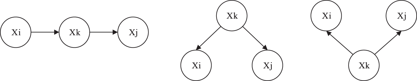
Three special node connection situations.

The purpose of structure learning is to find out the dependencies between nodes and then construct a network structure model corresponding to the training data set’s simulation state, which is learned by the entire BN method necessary steps. All subsequent analyses are based on the completion of the work.

For a set of random variables V = {V₁, V₂, . . . , V_n} and the training data set D = {D⁽¹⁾, D⁽²⁾, . . . , D^(m)} about these variables, where m is the number of training sets. The goal of learning is to obtain the most adaptable DAG structure G. When there are few variables and fewer iterations, it is easy to get the structure. However, when the number of nodes is large, the corresponding graph structure’s complexity will increase accordingly. The number of DAG g(n) and the number of nodes n satisfy the function (4): $g (n) = {\begin{matrix} 1, n = 1 \\ \sum_{i = 1}^{n} (- 1)^{i + 1} C_{n}^{i} 2^{i (n - i)} g (n - i), n > 1 \end{matrix}$ (6)

According to the algorithm difference of structure learning, different types can be extended. In essence, these methods are mainly divided into two categories: constraint-based methods and search score-based algorithms. The following specific search scored-based methods are utilized in this study.

(i) Algorithm based on search score

The search-and-score-based BN structure learning algorithm mainly proposes optimization and improvement schemes through BN and uses existing scoring algorithms to calculate the highest-scoring network structure [12]. The structure learning model of search scoring can be uniformly expressed as the function model: ${\begin{matrix} max f (G, D), \\ s . t . G \in ϑ, G | = C, \end{matrix}$ (7)

Where f is the core formula, i.e., the search scoring function, θ is the structure learning space, and G| = C means that the directed acyclic graph G satisfies the constraint C. In the search scoring system, the restriction C is to ensure that the searched model structure is all DAG. The optimal structure can be expressed as the function: $G^{*} = \underset{G}{arg max} (G, D)$ (8)

In machine learning, we must first determine the training set D and the potential structure G, and penalize the data that does not meet the requirements and the results that have the properties of the DAG graph structure. In addition, when the structure meets the data distribution requirements, give the graph structure a simple Higher evaluation of the model. If the scoring algorithm’s calculation results have better homogeneity, it means that the results also have higher sufficient accuracy. Based on this situation’s consideration, the scoring function is further classified into Bayes-based and information-based scoring functions. The research process of this paper uses Bayes-based scoring functions. The Bayesian scoring function regards the formula G^* as a MAP type problem: $G^{*} = \underset{G}{arg max} (G | D)$ (9)

Where P (G|D) is the posterior probability of structure G given D. Assuming that the prior probability of g is P (G), according to Bayesian formula: $P (G | D) = \frac{P (D | G) P (G)}{P (D)}$ (10)

P (D) has nothing to do with g, so P (G|D) is proportional to P (D|G) P (G), and the logarithm of both sides are: $log P (G | D) = log P (D | G) + log P (G)$ (11)

If the parameter of the directed acyclic structure G is ΘG, we can get: $P (D | G) = \int_{Θ G} P (D | G, Θ G) P (Θ G | G) d Θ G$ (12)

Where the likelihood function L (G, ΘG|D) P (D|G, ΘG) represents the relevant number set of the structural model. In the process of analyzing the discretized training set, it is generally assumed that the prior probability distribution P (ΘG|G) of the model parameters obeys the Dirichlet distribution probability with the parameter α_ijk: $P (Θ G | G) = \frac{Γ (α_{ij})}{\sum_{k = 1}^{r_{i}} Γ (α_{ijk})} \prod_{k = 1}^{r_{i}} θ_{ijk}^{α_{ijk} - 1}$ (13)

Where Γ represents the gamma function, r_i is the number set of training objects whose state of the node V_i is k and the parent node combination is j, m_ij = ∑_km_ijk and α_ij = ∑_kα_ijk. Combining formula (6) with (10) can get:

$\begin{matrix} log P (G | D) = \sum_{i = 1}^{n} \sum_{j = 1}^{q_{i}} \\ (log \frac{Γ (α_{ij})}{Γ (α_{ij} + m_{ij})} \sum_{k = 1}^{r_{i}} log \frac{Γ (α_{ijk} + m_{ijk})}{Γ (α_{ijk})}) + log P (G) \end{matrix}$ (14)

This formula is also called the BD score. When the structure is equal frequency distribution, log P (G) =0, the latter term of the BD score can be ignored, which is called the GH score [13].

Regarding the Dirichlet parameter α_ijk, it exists in the BD score. If the Dirichlet parameter α_ijk obeys 1, the K2 score is derived. This article mainly employs the K2 scoring model:

$\begin{matrix} f_{K 2} (G, D) = \sum_{i = 1}^{n} \sum_{j = 1}^{q_{i}} \\ (log \frac{(r_{i} - 1)!}{(m_{ij} + r_{i} - 1)!} \sum_{k = 1}^{r_{i}} log m_{ijk}!) + log P (G) \end{matrix}$ (15)

(ii) K2 algorithm

The K2 algorithm is a scoring function, as described above, is a structure learning algorithm. It was first proposed by Cooper and Herskovits [16]. In the algorithm, the quality of the structure is measured by the CH score. To limit the search space, the node order ρ and a positive integer u are used. The starting point of the K2 algorithm is a graph with unstructured and undirected lines. It traverses each node in turn according to the order of each node specified in the node sequence array and calculates its CH score by comparing the specific changes after a certain node is added. If it increases the representative, it is necessary to increase the parent node. To avoid the parent node’s redundancy, limiting the number of parent nodes is mainly by using a positive integer u. However, identifying the proper node sequence is the most basic part of the algorithm, and the final output network structure diagram is closely related to the difference in node sequence. Therefore, the K2 algorithm is so widely used. Experts and scholars have proposed various solutions to the problem of node order improvement, such as the method of learning node order, which is completed by the CI test.

2.3 Model reliability evaluation

In analyzing the research influence relationship, Chen Yanyan et al. [26] used logistic regression analysis to distinguish and analyze the road traffic influence factors; Yu et al. [7] used spatiotemporal recurrent convolutional networks to predict large-scale transportation network traffic. To verify the BN’s effectiveness, Zhang et al. [3] utilized the ROC area, accuracy, and other indicators in the comparative analysis of the BN, decision tree, support vector machine, and other algorithms to construct the traffic accident black spot recognition model. This section also uses the following indicators for model reliability evaluation.

ROC area is enclosed by the coordinate axis under the ROC curve, the decimal of the range of [0, 1]. The ROC curve is generally compared with y = x. The area above the linear function graph is usually above 0.5. The closer this value is to 1, the better the effect of the model. The value in [0.5, 0.7] is lower accuracy, [0.7, 0.9] represents a certain degree of accuracy, [0.9, 1] represents better accuracy, and [0, 0.5] represents completely invalid. The true positive rate (TP) rate measurement sensitivity is defined as the ratio of actual positive and predicted positive samples. The false positive rate (FP) rate represents the proportion of actual negative and predicted positive samples. The ratio of the TP rate to the FP rate is directly proportional to the classification effect. The larger the ratio, the better the effect.

Precision is the proportion of samples that are predicted to be positive if they are positive.

Recall is a measure of coverage, which is equal to sensitivity.

F-measure is used to comprehensively evaluate precision and recall indicators. When the F metric is larger, the effect of the classifier is better.

Accuracy is often used when testing the classification effect—the greater the accuracy, the better the classifier’s performance.

The calculation formula for each index is as follows. $TPR = \frac{TP}{TP + FN}$ (16) $FPR = \frac{FP}{FP + TN}$ (17) $Pr ecision = \frac{TP}{TP + FP}$ (18) $Re call = \frac{TP}{TP + FN}$ (19) $F - measure = \frac{2 TP}{2 TP + FP + FN}$ (20) $Accuracy = \frac{TP + TN}{TP + TN + FP + FN}$ (21)

Where TP is actually positive and predicted positive data, FP is actually negative but predicted positive data, TN is actually negative and predicted negative data, FN is actually positive but predicted negative data.

3 Impact of subway on urban traffic

3.1 Collection of influence indicators based on GRA

The evaluation system to explore the impact of subway opening on urban transportation development is divided into three layers: cause layer, first-level indicators layer, and second-level indicators layer. The first layer is the cause layer, whether to build a subway is the criteria; the second layer is the main content of the evaluation system, setting sub-goals from three aspects: accessibility, green transportation, and safety; the third layer is the second-level indicators layer and indicators at this level are all numerical indicators. There are 22 indicators in the second-level indicators layer, shown as Table 3. The statistical data of each reference sequence from 2008 to 2018 is shown in Table 4.

Table 2
K2 algorithm

Step

1 input: Training set D, Node order ρ, Positive integer u

2 output: Directed acyclic graph G

3 Identify node set V from D, let E = {};

4 For i = 1 to n do

5 Pa(Vi)=Φ;

6 Pold = fch((Vi, Pa(Vi)),D);

7 findmore = true;

8 While findmore and |Pa(Vi)|<u do

9 Z← The node that maximizes Fch((Vi,Pa(Vi)∪Z),D) in Pred(Vi)¥pa(Vi);

10 Pnew = Fch((Vi,pa(Vi)∪ Z),D);

11 If Pnew > Pold then

12 Pold = Pnew;

13 Pa(Vi)=Pa(Vi)∪ Z;

14 Else findmore = false;

15 end

16 end

17 end

Step
1	input: Training set D, Node order ρ, Positive integer u
2	output: Directed acyclic graph G
3	Identify node set V from D, let E = {};
4	For i = 1 to n do
5	Pa(Vi)=Φ;
6	Pold = fch((Vi, Pa(Vi)),D);
7	findmore = true;
8	While findmore and \|Pa(Vi)\|<u do
9	Z← The node that maximizes Fch((Vi,Pa(Vi)∪Z),D) in Pred(Vi)¥pa(Vi);
10	Pnew = Fch((Vi,pa(Vi)∪ Z),D);
11	If Pnew > Pold then
12	Pold = Pnew;
13	Pa(Vi)=Pa(Vi)∪ Z;
14	Else findmore = false;
15	end
16	end
17	end

Table 3

Primary selection index system table

Cause layer	First-level indicators layer	Second-level indicators layer	Variable name
Whether the	Accessibility	Growth of per capita traffic network area	X1
subway is open		Growth rate of bus operating mileage	X2
		Road area growth rate	X3
		Number of buses per 10,000 people	X4
		Citizen travel coefficient	X5
		Total bus passenger transport	X6
		Proportion of land consumption for urban transportation	X7
		Taxi growth	X8
		Total taxi passenger transport	X9
	Green transportation	Growth rate of car ownership	X10
		Increase in green coverage	X11
		Infrastructure investment	X12
		Annual average concentration of inhalable particulate matter	X13
		Percentage of primary electric energy	X14
		Road cleaning area	X15
		Energy consumption elasticity coefficient	X16
	Safety	Proportion of drivers with driving experience under three years	X17
		Accident rate per 10,000 vehicles	X18
		Death rate per 10,000 vehicles	X19
		Death rate per hundred kilometers	X20
		Average economic loss from traffic accident	X21
		Number of road traffic accidents	X22

Table 4

Statistical Table of Reference Sequences from 2008 to 2018

	2008	2009	2010	2011	2012	2013	2014	2015	2016	2017	2018
x1	8.38	7.82	11.01	11.24	14.83	15.46	16.59	16.94	17.25	18.18	19.51
x2	–185	693	1961	465	67	–113	134	554	383.8	282.7	1486
x3	4.97	3.81	6	6.57	7.24	6.6	6.89	7.32	9.34	9.72	9.33
x4	17.43	16.2	15.56	19.07	22.07	19.04	17.35	12.1	12.2	13.9	14.2
x5	2.49	2.54	2.53	2.59	2.59	2.49	2.49	2.49	2.59	2.67	2.68
x6	3538	52560	53918	59248	60538.5	60369	61773	62572.7	43010	40865.6	38832.3
x7	7.99	7.42	10.37	10.75	14.38	10.48	11.14	12.22	16.06	15.3	15.3
x8	76	79	61	532	408	457	221	214	2	0	2
x9	340	9894	16652	18135	19394.4	18935.1	20778	23965.1	20224.9	19764.9	18715.1
x12	62600	120866	112894	167582	761098	629528	527411	491755	500561	548458	567927
x14	4.7	4.7	4.1	6.8	5.4	5.4	7.4	7.5	8.1	7.5	7.3
x15	2333	2333	2447	2095	2919	2051	2884	3099	4421	4415	4964
x17	36.23	33.34	23.22	22.98	22.67	22.34	22.3	22.35	22.51	17.01	15.86
x18	15.08	10.29	7.87	5.82	3.98	4.33	4.37	1.4	1.5	1.2	1.1
x19	20.71	14.3	10.85	8.58	6.05	6.24	6.95	2.66	2.73	2.59	2.36
x20	4752	5312.7	5742	6086	6477	6865	7250	8185	8977	10289	11222
x21	0.16	0.21	0.23	0.19	0.28	0.18	0.21	0.54	0.36	0.28	0.3
x22	5917	4262	4126	3354	3112	2880	2873	3014	2316	2369	1823

The calculated correlation degree is shown in Table 5. The second-level indicators under the first-level accessibility index have a large correlation with subway opening. The maximum is the growth rate of road area rate X3 reaching 0.975678726, and the minimum is taxi operation. The increase in the number of vehicles X6 is 0.648601097, while the correlations of the secondary indicators under the green transportation primary indicators are relatively small. The maximum is the road cleaning area X15, and the minimum is the energy consumption elasticity coefficient of only X16, which is 0.433484404, and the accessibility is level 1. For each secondary index under the index, the maximum X20 reaches 0.934185223, and the minimum X18 reaches 0.682965801. When Ma Xiaotong [25] analyzes the influencing factors related to single-vehicle accidents using improved grey correlation analysis, the factors with the average correlation degree exceeding 0.6 are selected as the key factors affecting the occurrence of the accident. Therefore, in this section, indicators with a correlation degree greater than 0.6 are selected as the evaluation indicators for the impact of subway opening on urban traffic, so X1, X2, X3, X4, X5, X6, X7, X8, X9, X12, X14, X15, X17, X18, X19, X20, X21, X22 are used as traffic indicators for follow-up analysis.

Table 5

Grey correlation degree of each comparison sequence

X1	X2	X3	X4	X5	X6
0.9963	0.9977	0.9964	0.9937	0.9949	0.9927
X7	X8	X9	X10	X11	X12
0.9962	0.6486	0.9953	0.5128	0.5431	0.6844
X13	X14	X15	X16	X17	X18
0.5207	0.6035	0.6712	0.4335	0.8557	0.6830
X19	X20	X21	X22
0.7448	0.9342	0.9192	0.8288

3.2 Influence model based on Bayesian networks

From the BN structure (Fig. 4), it can be seen that the per capita traffic network area growth X1 and the bus operation mileage growth X2 are only dependent on the opening of the subway. However, the four indicators of road area rate growth rate X3, infrastructure investment X12, taxi operating vehicle number growth X8, and total bus passenger transport X6 are not only directly affected by the opening of subways, but also by per capita traffic network area growth X1 and bus operations mileage increase X2. In addition, the proportion of urban transportation land consumption X7, road cleaning area X15, 100-kilometer road death rate X20 related to not only the opening of the subway, but also one of the increases in the traffic network area per capita X1, the increase in bus operating mileage X2, the road area rate growth rate X3, infrastructure investment X12, and taxi operating vehicle number growth X8 and total bus passenger transport X6. Moreover, the number of standard buses for 10,000 people X4, the travel coefficient of citizens X5, the proportion of one-time electric energy X14, the accident rate of 10,000 vehicles X18, and the total number of taxi passengers X9 not only related to the opening of the subway, but also two of the increase in traffic network area per capita X1, the increase in bus operating mileage X2, the increase in road area rate X3, the infrastructure investment X12, the increase in the number of taxi operations X8, and the total number of bus passenger transport X6. Furthermore, the proportion of drivers under three years of driving experience X17, the death rate per 10,000 vehicles X19, the average economic loss of traffic accidents X21, and the number of road traffic accidents X22 are not only directly related to the opening of the subway, but also other 14 attribute variables.

Fig. 4

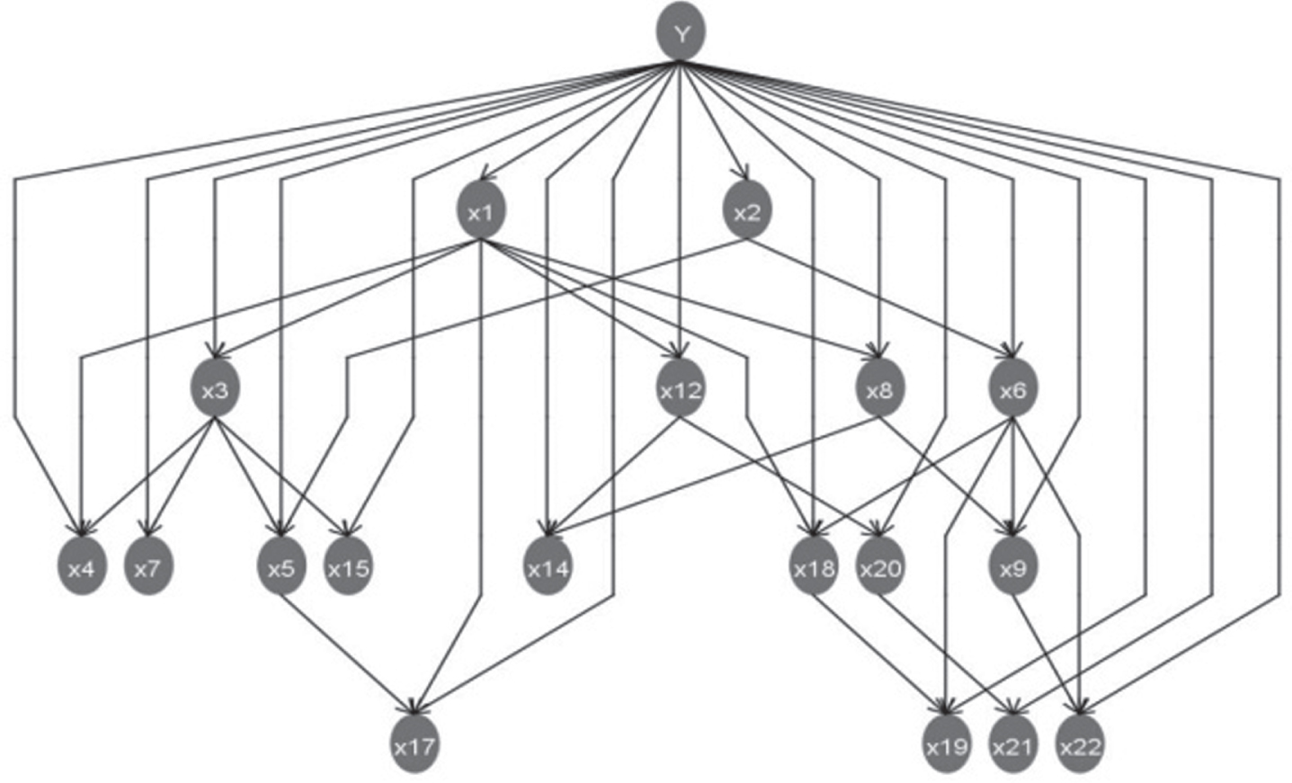
The influence of subway opening on urban traffic Bayesian networks structure.

To judge the reliability of selecting GRA for index screening, under the condition of adopting the BN method, the result of analyzing 22 indexes without index screening with GRA is compared with the outcome of index screening using GRA. Moreover, in this paper, the ROC curve area is selected as the reference index for comparison. The ROC curve is shown in Fig. 5, where the abscissa represents the false positive rate, and the ordinate represents the true positive rate. Among them, the ROC curve area of GRA-BNs is 0.986, and the ROC curve area of All-BNs is 0.886. Therefore, it is better to use GRA to screen than to analyze 22 indicators without GRA.

Fig. 5

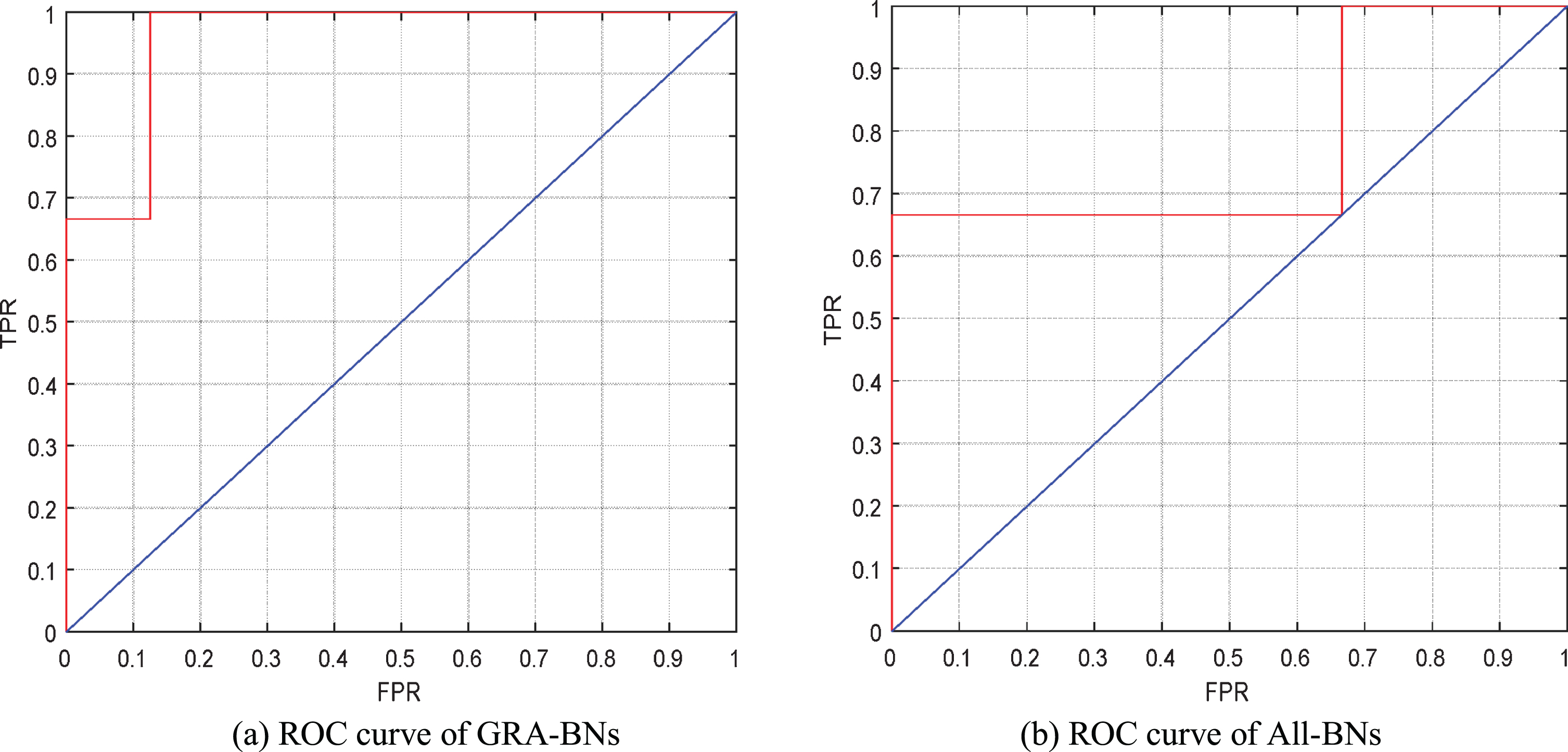
ROC curve graph of the full index and grey relational analysis.

To further explore the reliability of proposed GRA-BNs, the results are compared with the Naive Bayes Model (NBM) [14], Random Decision Forests (RDF) [20], and Logistic regression analysis (GLM) [19]. The ROC curve is shown in Fig. 6, where the abscissa represents the false positive rate, and the ordinate represents the true positive rate. In the three times of learning, the ROC area exceeded 0.5, so it shows that the learning results for the four models are all effective. Among them, the ROC curve area of GRA-NBM is 0.694, the ROC curve area of GRA-RDF is 0.771, and the ROC curve area of GRA-LGM is 0.664, which are all inferior compared with GRA-BNs (0.986).

Fig. 6

ROC curve.

Table 6 lists the other six indicators to evaluate GRA-BNs, All-BNs, NBM, RDF, and GLM. Among them, GRA-BNs has a precision of 1.000 and an accuracy of 0.958 as the optimal values, and All-BNs are the best values when the true positive rate reaches 1.000, the false positive rate reaches 0.667, and the recall rate reaches 1.000. In addition, the false positive rate of NBM reaches 0.667, which is also the optimal value for the false positive rate as All-BNs.

Table 6

Calculation table of each evaluation index

	TPR	FPR	Precision	Recall	F-Measure	ACC
GRA-BNs	0.875	0.557	1.000	0.875	0.810	0.958
All-BNs	1.000	0.667	0.75	1.000	0.857	0.500
NBM	0.833	0.667	0.714	0.883	0.769	0.189
RDF	0.875	0.333	0.875	0.875	0.875	0.542
GLM	1.000	0.333	0.889	1.000	0.941	0.770

As shown in Fig. 7, color blocks are used to visually show the pros and cons of the five learning sessions. Ideally, the higher the true positive rate to the false positive rate and the other four indicators, the better the learning result. In comparing the six indicators in this study, there is no low-level indicator in the learning results of GRA-BNs, while there is one low-level indicator in All-BNs, five low-level indicators for NBM, two low-level indicators for RDF, and two low-level indicators for GLM. Thus, in terms of low-level indicators, GRA-BNs is better.

Fig. 7

Comparison chart of 6 indicators.

4 Discussions and conclusions

After the model is built, each node’s conditional probability is learned, and the dependence between the variables is quantitatively described. This paper takes the influence of subway opening on urban traffic indicators as the research objective, so the probability distribution between each of the 18 attributes and the subway opening and other attribute variables is studied.

It can be seen from Table 7 that before the opening of the subway, the value of per capita traffic network area growth is evenly distributed in the four sections without obvious trend characteristics. Still, after the subway is opened, the probability that the per capita traffic network area increases above 16.5875 m2 will reach 70%; it can be judged that the annual increase in the traffic network area per capita has increased significantly after the opening of the subway.

Table 7

Conditional probability analysis results of per capita traffic network density increase number

Opening	(-inf-746.75]	(746.75–1493.50]	(1493.50–2240.25]	(2240.25–inf)
No	0.25	0.25	0.25	0.25
Yes	0.1	0.1	0.1	0.7

Table 8 illustrates that before the subway opening, the annual increase in bus operating mileage was mainly distributed above 16.5875 m2. After the subway opening, the annual increase in bus operating mileage was mostly less than 10.7425 km. There is a clear downward trend in the growth of operating mileage.

Table 8

Conditional probability analysis results of the increase of bus operating mileage

Opening	(-inf-10.7425]	(10.7425–13.665]	(13.665–16.5875]	(16.5875–inf)
No	0.05	0.10	0.35	0.50
Yes	0.85	0.05	0.05	0.05

Seen as Table 9, the per capita traffic network density growth is constant and higher than 16.5875 m2 when the subway is not opened, and the road area growth rate is concentrated in [6.77%, 8.24%], while the growth rate mostly exceeds 8.24% after the subway is opened. Therefore, the opening of the subway stimulated the increase in the growth rate of the road area.

Table 9

Conditional probability analysis results of road area rate growth rate

Opening	(-inf-5.2875]	(5.2875–6.7650]	(6.7650–8.2425]	(8.2425–inf)
No	0.125	0.125	0.625	0.125
Yes	0.1	0.1	0.1	0.7

It can be seen from Table 10 that when the per capita traffic network density increase is constant and is lower than 13.665 km. When the subway is not opened, the infrastructure investment is concentrated at less than 2,372.245 million yuan. After the subway is opened, the infrastructure investment is more flexible, with a balanced distribution in each interval.

Table 10

Conditions probability analysis results of infrastructure investment

Opening	(-inf-237224]	(237224–411849]	(411849–586474]	(586474-inf)
No	0.625	0.125	0.125	0.125
Yes	0.250	0.250	0.257	0.250

Table 11 shows that when the per capita traffic network density increase is constant and is higher than 16.5875 km. When the subway is not opened, the increase in the number of taxis operating is concentrated between 133 and 266. After the subway is opened, the increase in the number of taxi operating vehicles is concentrated below 133. Therefore, the subway opening has a significant negative impact on the growth of the number of taxis in Nanchang.

Table 11

Conditional probability analysis results of the increase in the number of taxi operating vehicles

Opening	(-inf-133]	(133–266]	(266–399]	(399-inf)
No	0.125	0.625	0.125	0.125
Yes	0.7	0.1	0.1	0.1

It can be seen from Table 12 that under the condition that the increase in bus operating mileage remains the same and is higher than 26388.775 km. When the subway is not opened, the total number of bus passengers is mainly distributed over 47814. After the subway is opened, the total number of bus passengers is mainly distributed between 33055 and 47814 people. Therefore, after the opening of the subway, the passenger traffic volume of Nanchang has decreased.

Table 12

Conditional Probability Analysis Results of Total Bus Passenger Transport

Opening	(-inf-18297]	(18297–33055]	(33055–47814]	(47814-inf)
No	0.056	0.056	0.056	0.833
Yes	0.167	0.167	0.500	0.167

Table 13 demonstrates that when the road area rate growth rate remains unchanged and is higher than 8.24%. When the subway is not opened, the proportion of urban traffic land consumption is evenly distributed in each section, and there is no obvious law. After the subway is opened, the proportion of urban traffic land consumption is mainly distributed above 13.9%. Therefore, after the subway opening, the proportion of urban transportation land consumption has increased significantly.

Table 13

Conditional probability analysis results of the proportion of urban traffic land consumption

Opening	(-inf-9.58]	(9.58–11.74]	(11.74–13.90]	(13.90-inf)
No	0.25	0.25	0.25	0.25
Yes	0.1	0.1	0.	0.7

Table 14 indicates that under the condition that the road area’s growth rate remains unchanged and is higher than 8.24%. When the subway is not opened, the road cleaning area is uniformly distributed in each section, and there is no obvious law. After the subway is opened, the road cleaning area is mainly distributed above 4235.75 m2. Therefore, after the opening of the subway, the road cleaning area has increased significantly.

Table 14

Conditional probability analysis results of road cleaning area

Opening	(-inf-2779.25]	(2779.25–3508.00]	(3508.00–4235.75]	(4235.75-inf)
No	0.25	0.25	0.25	0.25
Yes	0.1	0.1	0.1	0.7

It can be seen from Table 15 that under the condition that the infrastructure investment remains unchanged and is less than RMB 237,224.5 million, the average economic loss from traffic accidents before the opening of the subway is mainly distributed under RMB 63.695 million. After the opening of the subway, there is no obvious law in the distribution of average economic losses from traffic accidents.

Table 15

Conditional probability analysis results of average economic loss from traffic accidents

Opening	(-inf-6369.5]	(6369.5–7987.0]	(7987.0–9604.5]	(9604.5-inf)
No	0.750	0.083	0.083	0.083
Yes	0.25	0.25	0.25	0.25

Table 16 shows that the per capita traffic road network area growth rate is unchanged and higher than 16.5875 km2, and the road area growth rate is unchanged and higher than 8.24%. Before the subway is opened, there is no obvious law in the distribution of the number of buses per 10,000 people, and they are evenly distributed in each interval. After the subway is opened, the number of buses for 10,000 people is mainly distributed in 14.925/10,000 people. Therefore, after the opening of the subway, the number of buses per 10,000 people showed a downward trend.

Table 16

Conditional probability analysis results of the number of bus standards with 10,000 people

Opening	(-inf-14.5925)	(14.5925–17.0600)	(17.0600–19.5775)	(19.5775-inf)
No	0.25	0.25	0.25	0.25
Yes	0.7	0.1	0.1	0.1

It can be seen from Table 17 that under the condition that the road area growth rate is unchanged and higher than 8.24%, and the increase of bus operating mileage is unchanged and higher than 10594.325 km. Before the opening of the subway, there is no obvious law in the distribution of the citizen travel coefficient, and they are evenly distributed in each interval. After the subway is opened, the citizen travel coefficient is mainly distributed above 2.6325. Therefore, after the subway was opened, the travel coefficient of citizens increased.

Table 17

Conditional probability analysis results of citizen travel coefficient

Opening	(-inf-2.5375]	(2.5375–2.5850]	(2.5850–2.6325]	(2.6325-inf)
No	0.25	0.25	0.25	0.25
Yes	0.125	0.125	0.125	0.625

Table 18 indicates that when the increase in the number of taxi operating vehicles remains unchanged and is less than 133, and the infrastructure investment remains unchanged and remains between 411.49 million yuan and 5.86473 million yuan. Before the opening of the subway, there is no obvious law in the distribution of the primary electric energy, and they are evenly distributed in each interval. After the subway is opened, the proportion of primary energy is generally distributed above 7.1%. Therefore, after the opening of the subway, the proportion of primary electric energy has increased.

Table 18

Conditional probability analysis results of primary electric energy condition

Opening	(-inf-5.1]	(5.1–6.1]	(6.1–7.1]	(7.1-inf)
No	0.25	0.25	0.25	0.25
Yes	0.1	0.1	0.1	0.7

Table 19 demonstrates that when the per capita traffic road network area growth is constant and higher than 16.5875 km2 and the total number of bus passenger traffic is unchanged and distributed between 33,055 and 47,814; there will be 10,000 car accidents before the subway is opened. The rate distribution has no obvious regularity, and it is evenly distributed in each section. After the subway is opened and operated, the accident rate of 10,000 vehicles is mainly distributed below 4.60%. Therefore, the subway opening will help reduce the accident rate of 10,000 vehicles and improve urban traffic safety.

Table 19

Conditional probability analysis results of an accident rate of 10,000 vehicles

Opening	(-inf-4.595]	(4.595–8.090]	(8.090–11.585]	(11.585-inf)
No	0.25	0.25	0.25	0.25
Yes	0.7	0.1	0.1	0.1

It can be seen from Table 20 that when the growth of the number of taxis operating is constant and less than 133, and the total number of bus passengers is unchanged and distributed between 33,055 and 47,814, the total number of taxi passengers before the opening of the subway. There is no obvious regularity in traffic distribution, and it is evenly distributed in each section. After the subway is opened and operated, the total number of taxi passengers is mainly distributed over 18,058.83.

Table 20

Conditional probability analysis results of total taxi passenger traffic

Opening	(-inf-6246.28]	(6246.28–12152.0]	(12152.00–18058.83]	(18058.83-inf)
No	0.25	0.25	0.25	0.25
Yes	0.1	0.1	0.1	0.7

Table 21 shows that when the accident rate of 10,000 vehicles remains unchanged and less than 4.595%, and the total number of bus passengers remains unchanged and is distributed between 33,055 and 47,814, there is no obvious distribution of mortality among 10,000 vehicles before the subway is opened, and it is evenly distributed in each interval. After the subway is opened, the death rate of 10,000 vehicles is mainly distributed below 6.9475%. Therefore, the death rate of 10,000 vehicles after the opening of the subway has shown a downward trend, which is beneficial to the development of urban traffic safety.

Table 21

Conditional probability analysis results of death rate of ten thousand vehicles

Opening	(-inf-6.9475]	(6.9475–11.5350]	(11.5350–16.1225]	(16.1225-inf)
No	0.25	0.25	0.25	0.25
Yes	0.7	0.1	0.1	0.1

It can be seen from Table 22 that when the average economic loss of traffic accidents remains unchanged and is distributed between 7987 and 9604.5, before the opening of the subway, the death rate per 100 kilometers is mainly distributed above 0.445%, and after the opening of the subway, it is mainly distributed between 0.35% and 0.445%. Therefore, the opening of the subway is conducive to reducing the mortality rate of 100 kilometers of roads and is conducive to urban safety development.

Table 22

Conditional probability analysis results of the death rate of 100 kilometers of road

Opening	(-inf-0.255]	(0.255–0.350]	(0.350–0.445]	(0.445-inf)
No	0.167	0.167	0.167	0.500
Yes	0.167	0.167	0.500	0.167

Table 23 indicates that when the total number of taxi passengers is unchanged and higher than 18,058.825 and the total number of bus passengers is unchanged and distributed between 33,055 and 47,814, the distribution of the number of road traffic accidents before the opening of the subway. There is no obvious rule, and it is evenly distributed in each section. After the subway is opened, the number of road traffic accidents is mainly distributed below 2846.5. Therefore, the number of road traffic accidents after the subway opening shows a downward trend, which is beneficial to the development of urban traffic safety.

Table 23

Conditional probability analysis results of road traffic accidents

Opening	(-inf-2846.5]	(2846.5–3870.0]	(3870.0–4893.5]	(4893.5-inf)
No	0.25	0.25	0.25	0.25
Yes	0.7	0.1	0.1	0.1

This paper proposed a novel GRA-BNs method to analyze the impact of the subway operation on urban traffic. A three-layer framework is established, and 18 traffic indicators were comprehensively selected from 22 traffic indicators by considering three aspects: traffic accessibility, green traffic, and traffic security. To verify the proposed model, Bayesian Networks with full indicators analysis (All-BNs) and other three algorithms of the Naive Bayes Model (NBM), Random Decision Forests (RDF), and Logistic regression analysis (GLM) are employed to conduct the comparative analysis. The result shows that GRA-BNs is the most effective model to study the impact of the subway’s operation on urban traffic. In addition, the dependence relations between the subway and each index are analyzed by the conditional probability tables (CPTs), and some suggestions are given for the stakeholders. However, due to the objective circumstances with limited reference materials, there are still some limitations for this paper:

As the data collection in this article is mainly from the Jiangxi Statistical Yearbook and related traffic news reports on the Internet, the data’s completeness and comprehensiveness are lacking.

The preliminary consideration of urban traffic impact indicators is relatively one-sided. In terms of indicator selection, only accessibility, safety, and green transportation are considered. Still, many other factors have not been considered.

Since the Nanchang Metro opened in December 2015, the traffic data after the metro’s opening is relatively scarce, the analysis of the dependence between various indicators is relatively shallow, and many possible laws have not been unearthed.

Data availability

The data will be accessible upon request.

Conflicts of interest

The authors declare that they have no conflicts of interest.

Footnotes

Acknowledgments

This work was financially supported by the National Natural Science Foundation of China (51805169, 51708218, 52062014). This study is also supported by the Natural Science Foundation of Jiangxi Province 20202BABL212009.

References

Ziedan

and Brakewood

, Longitudinal Analysis of Light Rail and Streetcar Safety in the United States, Transportation Research Record2674(9) (2020), 83–95.

Baoping

, Xiangdi

, Yonghong

, et al., Application of Bayesian Networks in Reliability Evaluation[J], IEEE Transactions on Industrial Informatics (2018), 1–1.

Zhang

, Shu

and Yan

, A Novel Identification Model for Road Traffic Accident Black Spots: A Case Study in Ningbo, China[J], IEEE Access (2019), 1–2.

Barros

C.P.

and Dieke

P.U.C.

, Choice valuation of traffic restrictions:Noise, pollution, and congestion preferences, A note, Transportation Research Part D: Transport and Environment (2008), 347–350.

Lin

, Yang

and Gao

, VISSIM-based Simulation Analysis on Road Network of CBD in Beijing, China[J], Procedia – Social and Behavioral Sciences (2013), 96.

Gomes

and Gan

, A Bayen. A methodology for evaluating the performance of model-based traffic prediction systems, Transportation Research Part C: Emerging Technologies96 (2018), 160–169.

, Wu

, Wang

, et al., Spatiotemporal Recurrent Convolutional Networks for Traffic Prediction in Transportation Networks[J], Sensors (2017), 1–16.

Xue

, Van Gelder

P.H.A.J.M.

, Papadimitriou

, et al., Grey RelationalAnalysis ofEnvironmental Influencing Factors of Autonomous Ships’ Maneuvering Decision-Making, 2019 5th International Conference on Transportation Information and Safety (ICTIS) (2019), IEEE, 1447–1452.

Xue

, Van Gelder

P.H.A.J.M.

, Reniers

, et al., Multi-attribute decision-making method for prioritizing maritime traffic safety influencing factors of autonomous ships’ maneuvering decisions using grey and fuzzy theories, Safety Science120 (2019), 323–340.

10.

Xue Wu

, et al., Research on Decision-Making Factors of Ship’s Driving Behavior Based on Grey Relation Entropy Analysis Method, CICTP: Intelligence, Connectivity, and Mobility, American Society of Civil Engineers Reston, VA (2018), 2056–2065.

11.

Chan

J.W.K

and Tong

T.K.L

, Multi-criteria material selections and end-of-life product strategy: Grey relational analysis approach[J], Materials & Design28(5) (2007), 1539–1546.

12.

Zhu

M.M.

, Research on Structure Learning and Inference in Bayesian Networks[D], Xidian University (2013), 12–16.

13.

Doguc

and Ramirez-Marquez

J.E.

, A generic method for estimating system reliability using Bayesian networks[J], Reliability Engineering & System Safety94(2) (2017), 542–550.

14.

Kupervasser

, Quantitative Structure-Activity Relationship Modeling and Bayesian Networks:Optimality of Naive Bayes Model[J], Chapters (2019), 1–21.

15.

Caceres

, Sierra-Alonso

, Cuesta

C.E.

, et al., Improving Urban Mobility by Defining a Smart Data Integration Platform, IEEE Access (2020), 204094–204113.

16.

Aghdam

, Tabar

V.R.

and Pezeshk

, Some node ordering methods for the K2 algorithm[J], Computational Intelligence35(1) (2019), 42–58.

17.

Trojanek

and Gluszak

, Spatial and time effect of subway on property prices[C], Journal of Housing and the Built Environment33 (2018), 359–384.

18.

, Liu

, Li

, et al., Spatial and Temporal Dynamics of Urban Expansion along the Guangzhou-Foshan Inter-City Rail Transit Corridor, China, Sustainability10(3) (2018), 18.

19.

Jin

S.B.

and Lee

J.W.

, Study on Accident Prediction Models in Urban Railway Casualty Accidents Using Logistic Regression Analysis Model[J], Journal of the Korean Society for Railway20(4) (2017), 482–490.

20.

Dong

S.S.

and Huang

Z.X.

, A Brief Theoretical Overview of Random Forests [J], Integrated technology2(01) (2013), 1–7.

21.

Mark

and Abigail

L.B.

, Traffic related noise and air quality valuations: evidence from stated preference residential choice models[J], Transportation Research Part D: Transport and Environment (2004), 1–27.

22.

Seo

and Nam

H.K.

, Trade-off relationship between public transportation accessibility and household economy: Analysis of subway access values by housing size[J], Cities87(APR.) (2019), 247–258.

23.

Jie

, Chaozhong

, Zhijun

, et al., Modeling human-like decision-making for inbound smart ships based on fuzzy decision trees, Expert Systems with Applications115 (2019), 172–188.

24.

Wang

X.J.

, Subway capitalization effect in Beijing: Theory and evidence on the variation of the subway proximity premium[J], Papers in Regional Science96(3) (2017), 495–518.

25.

X.T.

, Research on the Impact of Serious and Extreme Traffic Accidents Based on Bayesian Network [D], Chang’an University (2018), 29–50.

26.

Chen

, Xiangnan

L.I.

, Sun

, et al., Identification method of factors affecting traffic accident based on Logistics[J], Transportation Technology and Economy20(05) (2018), 1–5.

27.

Miao

, Yao

, Ruan

, et al., Seismic response of shield tunnel subjected to spatially varying earthquake ground motions[J], Tunnelling and Underground Space Technology77(JUL.) (2018), 216–226.

28.

Wang

, Wang

and Ai

, Comparative study on effects of binders and curing ages on properties of cement emulsified asphalt mixture using gray correlation entropy analysis, Construction and Building Materials54 (2014), 615–622.