Decision-making for location of manufacturing bases in an uncertain demand situation

Abstract

Multi-site selection is a hot research issue for equipment manufacturing enterprises. With the development of smart industry, equipment manufacturing enterprises have entered the era of personalized and small batch manufacturing. Enterprises want to better meet customer needs and win competition, they must carry out scientific factory planning and site selection, so as to ensure quick response to the market. Based on this, this paper proposes a two-stage location selection model. Firstly, the method uses fuzzy numbers to express the demand size of demand points. Secondly, the distance factor is used as a criterion to select the candidate manufacturing bases with sufficient available resources. Next, the location model of enterprise manufacturing base is established which the goal of maximizing service efficiency and the constraints of time, cost and demand. Finally, a random numerical example is used to simulate the model, and lingo is used to solve it.

Keywords

Location decision service benefit uncertain demand multiple locations

1 Introduction

The problem of enterprise location has always been the research focus of scholars at home and abroad. Reasonable location of manufacturing base can not only improve the profitability of the enterprise and reduce the inventory risk of the company, but also improve the customer service level and satisfaction of the enterprise, so as to expand the competitive advantage of the enterprise [18]. As a long-term planning investment of an enterprise, which is one of the most critical and important decision-making issues for an enterprise’s production and operation [23]. Due to the many conflicting factors involved in the site selection decision-making process of an enterprise, it is difficult to select a site. The location of the new facility is a common challenge for almost all private and public sector companies in the world [17].

With the in-depth study of the optimization location problem by scholars at home and abroad, the existing optimization location method can effectively solve the manufacturing base location problem of determining demand and order [3 , 9]. Deterministic demand and order are often hypothetical conditions set up for better research. In the actual location process, enterprises often can not accurately predict the needs of customers in advance. Therefore, the research on the location of manufacturing base in the uncertain demand environment is more in line with the actual situation.

In this paper, a two-stage location decision model is proposed to solve the location problem of manufacturing base in an uncertain demand situation. The enterprise’s decision-making process involves the participation of multiple experts to predict the demand as accurately as possible. Due to the complexity of the forecast and the subjectivity of the individual, the evaluation result given by the decision-making expert is not an accurate number. Before the decision-making site is selected, it is necessary to use scientific methods to quantify its forecasted demand. In the first stage, according to the candidate manufacturing base’s ability to acquire its manufacturing raw materials, the viable candidate manufacturing base with strong resource acquisition capability is selected. In the second stage, a decision model for manufacturing base selection is established with time, cost and service level as constraints, and the goal of maximizing service efficiency. Finally, the paper uses random values to simulate the proposed model, which verifies the feasibility and scientificity of the model. It provides a reference for the decision-making of the location of the manufacturing base of the enterprise under the situation of uncertain demand, and provides important assistance for the actual decision-making.

2 Literature review

Regarding the site selection decision of the manufacturing base, not only the construction cost and time issues, but also the operation and service issues, such as excessive transportation costs and quality loss, should be considered [1]. Therefore, the problem of manufacturing base is a decision-making problem with multiple criteria and schemes.

Aktas considered the continuity of users’ energy demand and the pollution of energy transmission, proposed a method of integrating analytic hierarchy process and similar ideal solution sorting technology [5]. Anvari and Turkay considered the impact of economic, environmental and social factors on sustainable development, and proposed a decision support framework for facility location based on the real data attributes of the Turkish digital product supply network. This framework promotes corporate social responsibility and shows new trends in business practice. Decision makers can make better social and environmental benefits under the premise of meeting the economic goals of the enterprise [20]. Liu has proposed a new method for location selection of public transportation hubs that takes into account both quantitative and qualitative factors. This method is a multi-attribute group decision-making method based on TOPSIS (Technique for Order Preference by Similarity to Ideal Solution) and deviation. It takes the number of passengers as a random variable in the model and applies stochastic programming theory to solve the model [21]. Mohamed gaved a fuzzy hierarchical location model in 2016 considering the relationship between location and political, economic, environmental and social factors [14]. In 2017, he combined on-line analytical processing and geographic information system to study the site selection of Landfill of Industrial Wastes (LIW), simulated his algorithm by taking the location of LIW in Morocco as an example [12]. Kaveh believed that the population flow factor is an indispensable consideration in the actual location problem, so a new genetic algorithm, geospatial information system and multi-criteria decision-making integration model are given to select the appropriate location for the hospital [15]. Özmen thinks that logistics center is the center of a specific region and puts forward a three-stage method of logistics center location framework in the context of Kayseri’s logistics development plan [16]. Considering the mixed uncertainty of actual location decision information, Guan proposed a hybrid multi-attribute decision-making method without information conversion and applied this method to the location model of earthquake emergency service database [24,25, 24,25]. Liu proposed a new MAGDM (Multi-Attribute Group Decision-Making) technology to solve the problem of plant location with complex interrelation structure by considering multiple alternatives and complex relationship patterns among multiple attributes [27]. Ayyildiz Aimed at the problem of gas station location, a new spherical fuzzy AHP comprehensive spherical WASPAS method was constructed under the fuzzy environment. This method was used to analyze the location problem of Istanbul gas station [7]. Ali Karaşan proposed a decision method based on intuitionistic fuzzy sets for the location selection of charging stations, which took into account some of the conflicts in the life cycle of charging bicycles [4].

In the existing research results, most of the literature research on the location decision-making problem follows the research paradigm of “demand determination, candidate position is known, model decision”. At present, more and more scholars pay attention to the discrepancy between the hypothesis of demand determination and the actual problem. The research under uncertainty plays an important role in decision-making. Considering that traditional location selection methods can no longer be used to solve such problems in uncertain demand situation. This paper proposes a two-stage decision-making model for the selection of manufacturing bases in an uncertain demand situation, which makes the manufacturing base selection more practical and more scientific and effective.

3 Problem description and symbol introduction

The existing researches on the location of manufacturing bases of enterprises mostly focus on the situation of demand determination. This type of decision-making model can effectively solve the problem of enterprises location under the customer needs are known. However, there are many forms of subjective and objective uncertainties in the actual location problem [19]. In view of the decision-making location of the enterprise manufacturing base under the situation of uncertain demand, this paper presents the logic model of location selection as shown in Fig. 1, which involves three entities: manufacturing resource raw material supply point, enterprise manufacturing base, and product demand point. Supply points supply raw materials needed for manufacturing base. The manufacturing base is responsible for converting raw materials into required products. The demand point is the sum of the demand for products in a region, which is responsible for delivering the products to various customers according to the demand. This paper does not consider the direct distribution between supply point and demand point. It is assumed that the locations of demand points and supply points are known and fixed, the alternative addresses for enterprises to build or expand manufacturing bases are known, and the supply capacity of raw materials at each supply point is known, but the demand at demand points is uncertain. Considering the uncertain demand of demand point, the location of manufacturing base is decided, aiming at the maximization of service efficiency.

Fig. 1

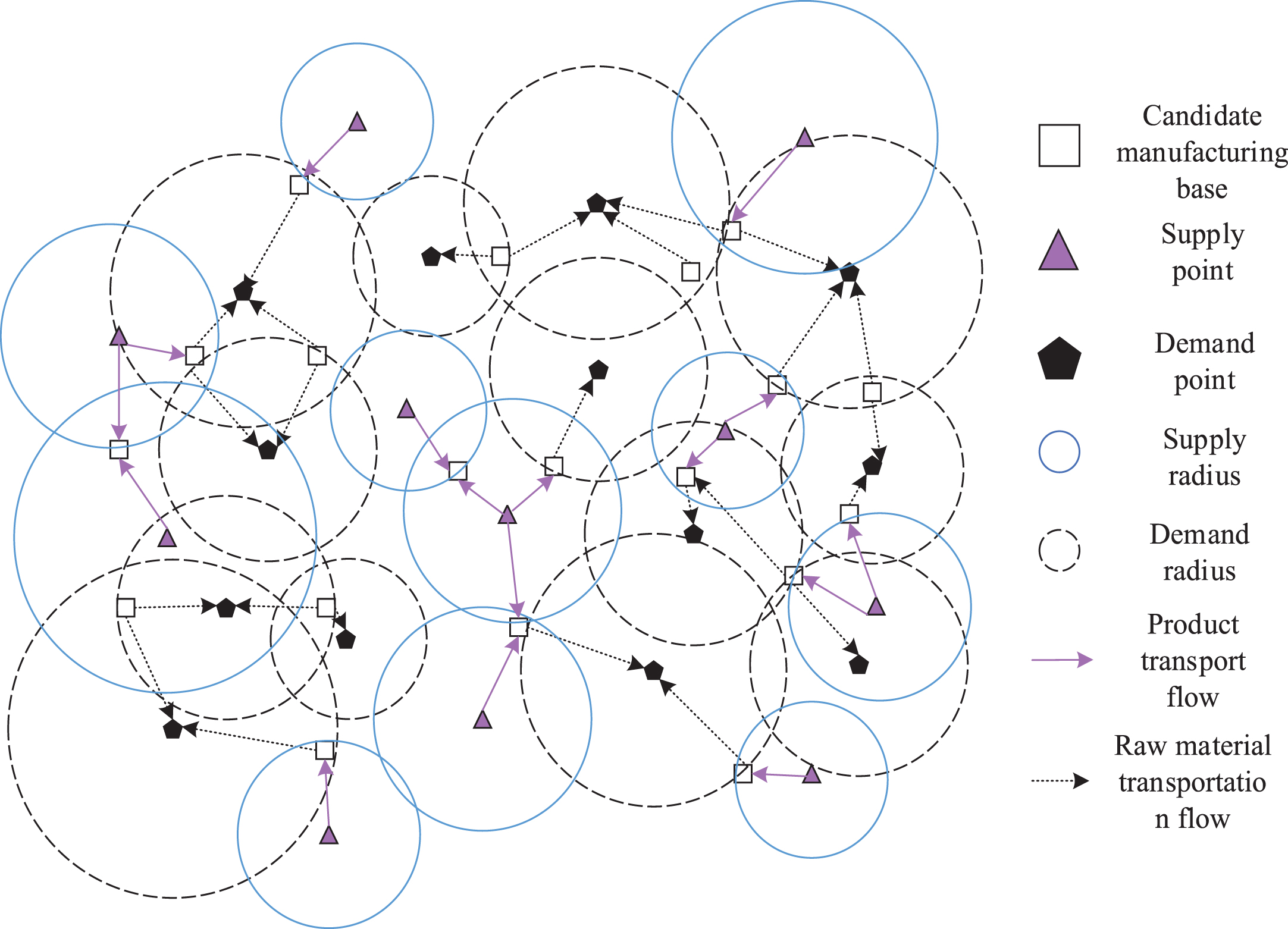
Logical model of manufacturing base location.

S ={ S₁, S₂, . . . , S_s }: A collection of supply points which supply raw materials. Where S_i is the i-th supply point, i = 1, 2, . . . , s.

M ={ M₁, M₂, . . . , M_m }: A collection of candidate manufacturing bases. Where M_j is the j-th candidate manufacturing base, j = 1, 2, . . . , m.

D ={ D₁, D₂, . . . , D_d }: A collection of demand points. Where D_l is the l-th demand point, l = 1, 2, . . . , d.

R ={ R₁, R₂, R₃, R₄ }: An expert collection of demand forecast for demand point. Where R_r is the r-th expert, r = 1, 2, 3, 4. This paper selects experts from 2 markets and 2 companies with senior working experience to form an expert group to predict the demand of demand points.

Q ={ Q₁, Q₂, . . . , Q_s }: A collection of available resources at supply points. Where Q_i is the available resources of the raw material supply point S_i, i = 1, 2, . . . , s.

O ={ O₁, O₂, . . . , O_d }: A collection of product demands. Where O_l is the demand for product from demand point D_l, l = 1, 2, . . . , d.

p_ij: The distance between the raw material supply point S_i and the company’s candidate manufacturing base M_j.

$p_{jl}^{*}$ : The distance between the company’s candidate manufacturing base M_j and the product demand point D_l.

4 Model introduction

4.1 Demand analysis based on triangular fuzzy numbers

Due to the complex and ever-changing market demands, it is difficult for enterprises to accurately predict the market demand. Demand analysis of demand points is extremely critical for the location of manufacturing bases [26]. If the forecast of demand is too low to meet the demand for products at the demand point, it is easy to cause delivery interruption or delay and bring sunk costs; If the demand forecast is too high, it may lead to oversupply, resulting in increased inventory costs caused by the backlog of goods. This paper discusses the location model of manufacturing bases in uncertain environments where market customer needs are vague. The common research methods of uncertainty are expected value method [6], chance constraint method [2], fuzzy function method [10]. Due to the complexity and subjectivity of demand forecasting and the uncertainty of the source of judgment, the evaluation results given by decision experts are not a clear number in essence, may be a fuzzy set of language terms or labels. Therefore, this paper uses the trigonometric function method to quantify the fuzzy language, so as to realize the forecast analysis of the demand at the demand point [13]. This method allows decision-making of estimated values under incomplete, inaccurate or uncertain information, and can compare the demand size of demand points to obtain a clear maximum or minimum order from the global ambiguity.

According to the method, firstly, each expert makes demand forecast for each demand point. The demand forecast value of each demand point is recorded as $A = [a_{lr}]_{d \times 4}$ (1)

a_lr represents the demand forecast value of demand point D_l given by expert R_r. Here, $a_{lr} = (a_{lr}^{L}, a_{lr}^{M}, a_{lr}^{R})$ is a triangular fuzzy number, $a_{lr}^{L}$ and $a_{lr}^{R}$ are the upper and lower bounds of the triangular fuzzy number, $a_{lr}^{M}$ is the median value between $a_{lr}^{L}$ and $a_{lr}^{R}$ , $a_{lr}^{L} < a_{lr}^{M} < a_{lr}^{R}$ . In order to reduce the influence of the subjective factors of the forecast results as much as possible, the experts predict that the language evaluation is used for demand forecast. The evaluation is shown in Table 1.

Table 1

Language evaluation level

Language evaluation	Symbol	Triangular fuzzy number
Very Low	VL	(0,1,2)
Low	L	(2,3,4)
Medium	M	(4,5,6)
High	H	(6,7,8)
Very High	VH	(8,9,10)

According to the demand forecast value(a_l1, a_l2, a_l3, a_l4) of demand point D_l given by the expert group. The value of fuzzy synthetic of demand point D_l is defined as $V_{l} = \sum_{r = 1}^{4} a_{lr} \times \frac{1}{\sum_{l = 1}^{d} \sum_{r = 1}^{4} a_{lr}}$ (2)

The value of $\sum_{r = 1}^{4} a_{lr}$ and $\sum_{l = 1}^{d} \sum_{r = 1}^{4} a_{lr}$ can be obtained by fuzzy addition algorithm. The Equations (3)–(4) is as follows $\sum_{r = 1}^{4} a_{lr} = (\sum_{r = 1}^{4} a_{lr}^{L}, \sum_{r = 1}^{4} a_{lr}^{M}, \sum_{r = 1}^{4} a_{lr}^{R})$ (3) $\sum_{l = 1}^{d} \sum_{r = 1}^{4} a_{lr} = (\sum_{l = 1}^{d} \sum_{r = 1}^{4} a_{lr}^{R}, \sum_{l = 1}^{d} \sum_{r = 1}^{4} a_{lr}^{M}, \sum_{l = 1}^{d} \sum_{r = 1}^{4} a_{lr}^{L})$ (4)

$V_{l} = (a_{l}^{L}, a_{l}^{M}, a_{l}^{R})$ and $V_{k} = (a_{k}^{L}, a_{k}^{M}, a_{k}^{R})$ are two triangular fuzzy numbers of evaluation, r ≠ k, r∈ { 1, 2, 3, 4 }, k∈ { 1, 2, 3, 4 }. Let W (V_l ⩾ V_k) represent the possible degree of triangular fuzzy numbers V_l ⩾ V_k. W (V_l ⩾ V₁, V₂, . . . , V_k) is the possible degree that the triangular fuzzy number V_l is greater than or equal to triangular fuzzy numbers V_k. Let w_l represent the degree of demand which demand point D_l is superior to other demand points [23]. It can be calculated by Equations (5)–(7). $w_{l} = (V_{l} ⩾ V_{1}, . . ., V_{l - 1,} V_{l + 1}, . . ., V_{d})$ (5)

When $a_{l}^{M} < a_{k}^{M}$ , $W (V_{l} ⩾ V_{k}) = {\begin{matrix} \frac{a_{k}^{L} - a_{l}^{M}}{(a_{l}^{M} - a_{l}^{R}) - (a_{k}^{M} - a_{k}^{R})}, a_{k}^{L} > a_{l}^{R} \\ 0, other \end{matrix}$ (6)

When $a_{l}^{M} ⩾ a_{k}^{M}$ , $W (V_{l} ⩾ V_{k}) = 1$ (7)

Note W = (w₁, w₂, . . . , w_d) is the absolute demand of each demand point relative to other demand points. In order to better measure the degree of demand of each demand point relative to the others, furthermore, the relative demand W = (w₁, w₂, . . . , w_d) is normalized to obtain the relative demand $W^{*} = (w_{1}^{*}, w_{2}^{*}, . . ., w_{d}^{*})$ of each demand point. Where $w_{l}^{*}$ is the relative demand of demand point D_l, which can be obtained by Equation (8). $w_{l}^{*} = \frac{w_{l}}{\sum_{l = 1}^{d} w_{l}}$ (8)

Here, $w_{l}^{*}$ meets $\sum_{l = 1}^{d} w_{l} = 1$ , $0 ⩽ w_{l}^{*} ⩽ 1$ , l = 1, 2, . . . , d.

By investigating and investigating the previous transaction information, the overall demand O for products in the region is evaluated. The demand of each demand point can be obtained by Equation (9). $O_{l} = w_{l}^{*} \times O$ (9)

4.2 Analysis of available resources based on distance factor

In the existing research literature, the supply capacity of manufacturing base is defined as “all or nothing” and “single coverage”, that is to say, the expanded or newly built manufacturing base can only be covered within the service radius of the supply point, otherwise it will not be covered, and then, the supply point can only be covered by the latest expanded or newly built manufacturing base. However, there are obvious irrationalities in the practical application of this assumption. For example, It is planned to establish several hospitals in a city, with the hospital as the center and 3 miles as the service radius. According to the existing research hypothesis, the residents within the service radius are in the state of full coverage, while the residents outside the service radius are in the state of no coverage. However, the reality is that residents at 3.1 miles may go to the hospital, and residents at 2.9 miles may not fully go to the hospital. It can be seen that such a hypothesis can not accurately describe the actual situation. Based on this, this paper relaxes the coverage conditions of the existing research, selects the distance factor as the coverage research object, considers the gradual coverage and joint coverage of the supply point [11], and proposes the analysis of the available resources of the supply point based on the distance factor.

Joint coverage emphasizes that the service status enjoyed by customers is the sum of all service facilities. In this paper, it can be understood that the resource acquisition of a newly built or expanded manufacturing base is the sum of manufacturing resources of all resource supply points. Without considering the influence of other factors, the manufacturing base can obtain resources from all supply points, which is consistent with the actual production situation.

Gradual coverage is a decreasing function. As the distance increases, customers have a lower level of service perception. In the research of this paper, the resource supply capacity of the supply point adopts the gradual covering function, that is, between the newly built or expanded manufacturing base and the supply point, with the increase of the distance, its ability to obtain available resources gradually decreases. The decreasing relationship is recorded as g (.). The common types of progressive coverage functions are shown in Fig. 2.

Fig. 2

Common gradual coverage functions.

This paper uses the gradual coverage function of type b in Fig. 2 to give the available resource function of the supply point based on the distance factor, it can be expressed as Equation (10).

$g (p_{ij}) = {\begin{matrix} Q_{i}; p_{ij} ⩽ r_{1} \\ Q_{i} - p_{ij}; r_{1} < p_{ij} ⩽ r_{2} \\ 0; r_{2} < p_{ij} \end{matrix}$ (10)

Here, r₁ is the full coverage radius; r₂ is the maximum service perception radius.

4.3 Decision model based on service benefit

4.3.1 Analysis of influencing factors

According to the analysis of the purchasing, production, transportation, sales and other characteristics of the manufacturing enterprise, it can be seen that the three factors of cost, time, and service are the most important factors that affect the service efficiency. Influencing factors can be shown in Table 2.

Table 2
Analysis of influencing factors

Influencing factors Symbol

Cost factors Construction costs c ^*

Transportation costs c

Time factors Transportation time of raw materials t ¹

Distribution time of products t ²

Service factors Available resources at manufacturing base e ¹

Service level at demand point e ²

Influencing factors	Symbol
Cost factors	Construction costs	c ^*
	Transportation costs	c
Time factors	Transportation time of raw materials	t ¹
	Distribution time of products	t ²
Service factors	Available resources at manufacturing base	e ¹
	Service level at demand point	e ²

Cost factors mainly include the construction costs and transportation costs of the enterprise. the construction costs include land costs and plant costs; transportation costs mainly include raw material transportation costs and product transportation costs incurred during the production and operation process.

Time factors mainly include the transportation time of raw materials and the distribution time of products to ensure the timely arrival of raw materials and the timely distribution of products.

Service factors mainly consider two aspects of services. On the one hand, the available resources of raw material supply point meet the minimum available resources of each candidate manufacturing base; on the other hand, each demand point can enjoy the minimum service level.

The total cost of production and operation of the candidate manufacturing base M_j is the sum of construction costs and transportation costs, which the calculation formula is as follows $C_{j} = c_{j}^{*} + c_{j}$ (11)

Among them, the transportation cost includes raw material transportation cost c_ij and product distribution cost c_jl, and the corresponding calculation Equation (12) is as follows. $c_{j} = \sum_{i = 1}^{s} c_{ij} + \sum_{l = 1}^{d} c_{jl}$ (12)

In order to facilitate research, this paper stipulates that the unit transportation cost is the same and expresses it as $\overset{\land}{c}$ , then Equation (12) can be expressed as Equation (13). $c = \overset{\land}{c} (\sum_{i = 1}^{s} p_{ij} + \sum_{l = 1}^{d} p_{jl}^{*})$ (13)

The production and operation time of the candidate manufacturing base M_j is the sum of raw material transportation time and product distribution time, which can be expressed by Equation (14). $T_{j} = \sum_{i = 1}^{s} t_{ij}^{1} + \sum_{l = 1}^{d} t_{jl}^{2}$ (14)

In the research process of this paper, the form of transportation is vehicle transportation, assuming that the transportation time factor is not affected by other factors, only related to the distance factor. If the driving speed of the car is a constant speed h, then the production and operation time Equation (14) can be expressed by Equation (15). $T_{j} = \frac{\sum_{i = 1}^{s} p_{ij} + \sum_{l = 1}^{d} p_{jl}^{*}}{h}$ (15)

In the research process of this paper, the gradual coverage function and joint coverage method are used to study the available resources of its candidate manufacturing base. It is required that the available resources of each candidate manufacturing base must reach the minimum level of manufacturing resources, which is recorded as Z_j. The corresponding calculation Equations (16)–(17) is as follows. $e_{j}^{1} = \sum_{i = 1}^{s} g (p_{ij})$ (16) $\sum_{i = 1}^{s} g (p_{ij}) ⩾ Z_{j}$ (17)

In the same way, we used the same research method to study the effective service of the demand point. The sum of the services required by the manufacturing base to meet the minimum service requirements of each demand point, which is recorded as $Z_{l}^{*}$ . The corresponding calculation Equations (18)-(19) is as follows. $e_{l}^{2} = \sum_{j = 1}^{m} g (p_{jl}^{*})$ (18) $\sum_{j = 1}^{m} g (p_{jl}^{*}) ⩾ Z_{l}^{*}$ (19)

4.3.2 Decision model of manufacturing base

According to the production and operation of enterprise (purchasing, production, and sales), this paper divides the decision-making model of the enterprise’s manufacturing base into two stages, namely the feasibility site selection stage and the site selection decision stage. The first stage is the feasibility site selection stage, which needs to select the feasible candidate manufacturing bases with sufficient available resources from the massive candidate manufacturing bases according to the supply of resources at the supply point. The second stage is based on the first stage, considering the minimum demand, time, and cost constraints of each demand point, and the location decision model with the goal of maximizing service benefit.

Through Equations (16)–(17) to screen its massive candidate manufacturing base, the first stage of the feasibility site selection stage is obtained. According to the results of the first stage, the second stage of the site selection decision stage is established as follows. $max \begin{matrix} \end{matrix} U = \sum_{l = 1}^{d} O_{l} \sum_{j = 1}^{m} g (p_{jl}^{*}) x_{j}$ (20) $s . t . \begin{matrix} \end{matrix} \sum_{j = 1}^{m} g (p_{jl}^{*}) x_{j} ⩾ Z_{l}^{*}$ (21) $\sum_{j = 1}^{m} x_{j} (c_{j}^{*} + \overset{\land}{c} (\sum_{i = 1}^{s} p_{ij} + \sum_{l = 1}^{d} p_{jl}^{*})) ⩽ C$ (22) $x_{j} (\frac{\sum_{i = 1}^{s} p_{ij} + \sum_{l = 1}^{d} p_{jl}^{*}}{h}) ⩽ T_{j}$ (23) $Z_{l}^{*} ⩾ 0, C ⩾ 0, T_{j} ⩾ 0, O_{l} ⩾ 0$ (24) $c_{j}^{*} ⩾ 0, p_{jl}^{*} ⩾ 0, p_{ij} ⩾ 0, h ⩾ 0$ (25) $x_{j} = {\begin{matrix} 0; j notselected \\ 1; j selected \end{matrix}$ (26)

Among them, Equation (20) is a service level with a degree of demand point, that is, the service benefit of manufacturing base is the greatest. Equation (21) indicates that the effective service level of each demand point is not lower than the minimum service requirement. Equation (22) indicates that the total cost of a new and expanded manufacturing base are not higher than the enterprise cost budget. Equation (23) indicates that the sum of raw material transportation time and product distribution time for each new or expanded manufacturing base must not exceed the time constraints of each manufacturing base. Equations (24)–(26) represent the range of decision variables.

5 Example analysis

On the [0,100]×[0,100] plane, randomly generate 60 demand points, 30 supply points and 20 candidate manufacturing bases. The positional relationship between the three is shown in Fig. 3. The basic information of demand points is shown in Table 3. The supply quantity Q_i of each supply point is randomly generated on [200,300], the full coverage radius r₁ is randomly generated on [5, 15], and the maximum service perception radius r₂ is randomly generated on [20, 35], as shown in the Table 4 is shown. The resource requirement Z_j of each candidate manufacturing base is randomly generated on [500,1000], the fixed cost is randomly generated on [15000,20000], as shown in Table 5. Using LINGO software, the model is studied and analyzed on a computer with Intel Core i5-8250u CPU, 8.00 gb memory and 64 bit operating system.

Fig. 3

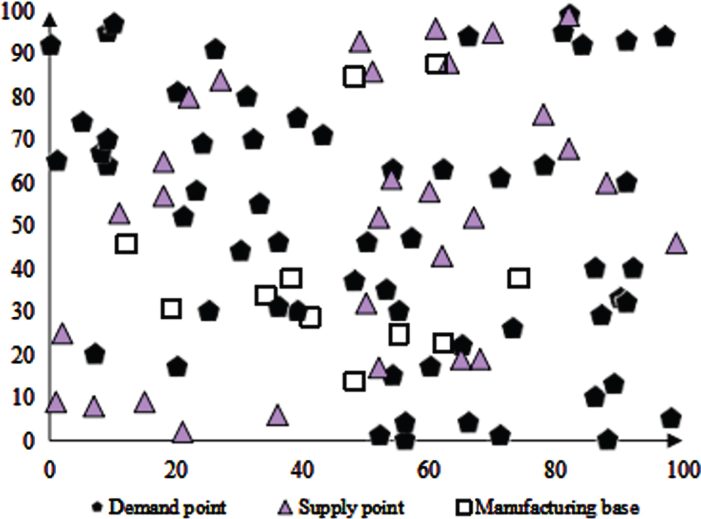
Location relationship of demand points, supply points and candidate manufacturing bases.

Table 3

Basic information of each demand point

D _l	Coordinate	D _l	Coordinate	D _l	Coordinate
1	(84,92)	21	(39,75)	41	(50,46)
2	(0,92)	22	(7,20)	42	(91,60)
3	(9,95)	23	(73,26)	43	(20,81)
4	(92,40)	24	(36,46)	44	(56,4)
5	(43,71)	25	(1,65)	45	(32,70)
6	(66,94)	26	(86,10)	46	(20,17)
7	(60,17)	27	(57,47)	47	(52,1)
8	(31,80)	28	(53,35)	48	(87,29)
9	(90,33)	29	(97,94)	49	(26,91)
10	(56,0)	30	(21,52)	50	(9,70)
11	(24,69)	31	(71,61)	51	(30,44)
12	(91,93)	32	(33,55)	52	(54,63)
13	(5,74)	33	(39,30)	53	(25,30)
14	(86,40)	34	(89,13)	54	(71,1)
15	(62,63)	35	(54,15)	55	(98,5)
16	(10,97)	36	(23,58)	56	(65,22)
17	(48,37)	37	(8,67)	57	(78,64)
18	(91,32)	38	(55,30)	58	(88,0)
19	(66,4)	39	(36,31)	59	(82,99)
20	(9,64)	40	(81,95)	60	(10,69)

Table 4

Basic information of each supply point

S _i	Coordinate	Q _i	r ₁	r ₂	S _i	Coordinate	Q _i	r ₁	r ₂
1	(63,88)	297	13	20	16	(22,80)	254	10	20
2	(52,17)	280	15	25	17	(11,53)	248	14	21
3	(61,96)	259	12	32	18	(67,52)	215	12	20
4	(68,19)	293	6	25	19	(27,84)	288	6	21
5	(82,99)	235	5	27	20	(65,19)	225	12	31
6	(51,86)	210	6	23	21	(88,60)	210	8	31
7	(1,9)	284	7	35	22	(70,95)	278	5	21
8	(78,76)	242	11	25	23	(82,68)	226	7	26
9	(7,8)	288	7	20	24	(50,32)	247	5	21
10	(49,93)	252	12	31	25	(21,2)	236	15	21
11	(36,6)	220	15	34	26	(54,61)	261	9	35
12	(52,52)	224	8	26	27	(15,9)	300	14	28
13	(18,65)	236	13	30	28	(60,58)	245	12	30
14	(18,57)	232	14	31	29	(2,25)	281	15	34
15	(99,46)	228	15	28	30	(62,43)	261	9	26

Table 5

Basic information of candidate manufacturing base

M _j	Coordinate	Z _j	C _j	M _j	Coordinate	Z _j	C _j
1	(61,88)	992	19656	11	(12,46)	668	19380
2	(29,6)	722	19284	12	(8,11)	820	19836
3	(19,31)	541	15722	13	(53,8)	839	15877
4	(55,35)	679	16415	14	(74,38)	573	16665
5	(94,76)	934	15317	15	(34,34)	985	17330
6	(73,16)	934	18351	16	(4,95)	878	17661
7	(73,85)	544	15056	17	(38,38)	964	15670
8	(41,29)	654	15361	18	(48,14)	521	18620
9	(48,85)	784	19684	19	(79,99)	566	17023
10	(84,93)	504	15481	20	(62,23)	623	15203

We hire 2 experts from the market and 2 experts from the company to form an expert group, use the language evaluation given in Table 1 to predict the demand of each point of demand, and then use the triangular fuzzy number to convert its language evaluation information into triangular fuzzy number, as shown in Table 6 (due to the large amount of data, the text only Show the specific data of 20 demand points).

Table 6

Demand forecast and evaluation (20 demand points)

D _l	Language evaluation information				Triangular fuzzy number
	R ₁	R ₂	R ₃	R ₄	R ₁	R ₂	R ₃	R ₄
1	H	VL	M	M	(6,7,8)	(0,1,2)	(4,5,6)	(4,5,6)
2	VL	M	VH	L	(0,1,2)	(4,5,6)	(8,9,10)	(2,3,4)
3	VH	VH	L	M	(8,9,10)	(8,9,10)	(2,3,4)	(4,5,6)
4	L	L	H	M	(2,3,4)	(2,3,4)	(6,7,8)	(4,5,6)
5	H	M	VH	VL	(6,7,8)	(4,5,6)	(8,9,10)	(0,1,2)
6	L	M	H	M	(2,3,4)	(4,5,6)	(6,7,8)	(4,5,6)
7	H	VL	H	M	(6,7,8)	(0,1,2)	(6,7,8)	(4,5,6)
8	M	VH	VH	L	(4,5,6)	(8,9,10)	(8,9,10)	(2,3,4)
9	M	VL	VH	VH	(4,5,6)	(0,1,2)	(8,9,10)	(8,9,10)
10	H	L	M	VH	(6,7,8)	(2,3,4)	(4,5,6)	(8,9,10)
11	L	M	L	M	(2,3,4)	(4,5,6)	(2,3,4)	(4,5,6)
12	M	M	VL	H	(4,5,6)	(4,5,6)	(0,1,2)	(6,7,8)
13	M	VH	H	H	(4,5,6)	(8,9,10)	(6,7,8)	(6,7,8)
14	L	VH	L	M	(2,3,4)	(8,9,10)	(2,3,4)	(4,5,6)
15	H	L	H	VL	(6,7,8)	(2,3,4)	(6,7,8)	(0,1,2)
16	H	VH	H	VH	(6,7,8)	(8,9,10)	(6,7,8)	(8,9,10)
17	VL	M	M	L	(0,1,2)	(4,5,6)	(4,5,6)	(2,3,4)
18	M	L	L	VH	(4,5,6)	(2,3,4)	(2,3,4)	(8,9,10)
19	M	VH	M	M	(4,5,6)	(8,9,10)	(4,5,6)	(4,5,6)
20	L	VH	M	VL	(2,3,4)	(8,9,10)	(4,5,6)	(0,1,2)

Hire 2 market and 2 companies, experts with senior work experience to form an expert group, use the language evaluation information given in Table 1 to predict the demand quantity of each demand point. Then we use triangular fuzzy numbers to transform those language evaluation information into triangle fuzzy number, as shown in Table 6. (Due to the large amount of data, only the specific data of 20 demand points are shown in the paper).

Through Equations (2)–(4), the weighted fuzzy comprehensive values of 20 demand points can be obtained, as shown in Table 7.

Table 7

Fuzzy comprehensive value of demand points (20 demand points)

D _l	$\sum_{r = 1}^{4} a_{lr}$	$\sum_{l = 1}^{d} \sum_{r = 1}^{4} a_{lr}$	Triangular fuzzy comprehensive value
1	(14,18,22)	(504,424,344)	(0.0278,0.0425,0.0640)
2	(14,18,22)		(0.0278,0.0425,0.0640)
3	(22,26,30)		(0.0437,0.0613,0.0872)
4	(14,18,22)		(0.0278,0.0425,0.0640)
5	(18,22,26)		(0,0523,0.0519,0.0516)
6	(16,20,24)		(0.0317,0.0425,0.0698)
7	(16,20,24)		(0.0317,0.0425,0.0698)
8	(22,26,30)		(0.0437,0.0613,0.0872)
9	(20,24,28)		(0.0397,0.0425,0.0814)
10	(20,24,28)		(0.0397,0.0425,0.0814)
11	(12,16,20)		(0.0238,0..0377,0.0581)
12	(14,18,22)		(0.0278,0.0425,0.0640)
13	(24,28,32)		(0.0476,0.0600,0.0930)
14	(16,20,24)		(0.0317,0.0425,0.0698)
15	(14,18,22)		(0.0278,0.0425,0.0640)
16	(28,32,36)		(0.0556,0.0755,0.1047)
17	(10,14,18)		(0.0198,0.0330,0.0523
18	(16,20,24)		(0.0317,0.0425,0.0698)
19	(20,24,28)		(0.0397,0.0425,0.0814)
20	(14,18,22)		(0.0278,0.0425,0.0640)

According to the above steps, the fuzzy comprehensive weight value of the demand point can be obtained. Based on this, the absolute weights of demand points are obtained according to Equation (5)–(7), and further, the relative weights of demand points are obtained by Equation (8). Assuming that the demand for products in this area is 10000, we can get the demand quantity of demand point, as shown in Table 8.

Table 8

The weight value and demand quantity of demand point

D _l	O _l	$w_{l}^{*}$	R	D _l	O _l	$w_{l}^{*}$	R	D _l	O _l	$w_{l}^{*}$	R
1	0.6194	0.0183	183	21	0.9889	0.0293	293	41	0.2247	0.0066	66
2	0.6194	0.0183	183	22	0.2884	0.0085	85	42	0.2444	0.0072	72
3	0.5996	0.0177	177	23	0.7252	0.0215	215	43	0.5470	0.0162	162
4	0.6194	0.0183	183	24	0.3006	0.0089	89	44	0.9531	0.0282	282
5	0.6039	0.0179	179	25	0.8763	0.0259	259	45	0.6422	0.0190	190
6	0.6137	0.0182	182	26	0.4175	0.0124	124	46	0.0940	0.0028	28
7	0.6137	0.0182	182	27	0.6511	0.0193	193	47	0.3286	0.0097	97
8	0.5996	0.0177	178	28	0.7665	0.0227	227	48	0.5288	0.0156	157
9	0.6039	0.0179	179	29	0.8098	0.0240	240	49	0.7846	0.0232	232
10	0.6039	0.0179	179	30	0.7190	0.0213	213	50	0.7476	0.0221	221
11	0.6911	0.0205	205	31	0.6881	0.0204	204	51	0.1074	0.0032	32
12	0.6194	0.0183	183	32	0.9739	0.0288	289	52	0.0136	0.0004	4
13	0.6875	0.0203	204	33	0.3132	0.0093	93	53	0.6706	0.0198	199
14	0.6137	0.0182	182	34	0.1522	0.0045	45	54	0.9123	0.0270	270
15	0.6194	0.0183	184	35	0.3973	0.0118	118	55	0.5328	0.0158	158
16	1.0000	0.0296	296	36	0.2417	0.0072	72	56	0.0918	0.0027	27
17	0.6326	0.0187	187	37	0.4876	0.0144	145	57	0.2097	0.0062	62
18	0.6137	0.0182	182	38	0.5802	0.0172	172	58	0.9290	0.0275	275
19	0.6039	0.0179	179	39	0.7124	0.0211	211	59	0.4912	0.0145	146
20	0.6194	0.0183	184	40	0.3470	0.0103	103	60	0.5042	0.0149	149

According to the basic information of the supply points given in Table 4, combined with Equation (10) and Equations (16)–(17), the number of available resources for each candidate manufacturing base can be calculated, as shown in Table 9. Further, according to the minimum resource requirements of manufacturing base given in Table 4. Candidate manufacturing bases are screened in the first stage to obtain the feasible site selection of manufacturing bases.

Table 9

Feasibility manufacturing base selection result table

M _j	Z _j	Q _i	S _i	Whether it is a feasible site?
1	992	1927	1,3,5,6,8,10,22,26	Yes
2	722	1246	7,11,14,27,29	Yes
3	541	1192	7,11,14,27,29	Yes
4	679	1427	2,4,10,20,24,30	Yes
5	934	840	5,8,21,23	No
6	934	770	2,4,20	No
7	544	2515	1,3,5,6,7,10,21,22,23,26,28	Yes
8	654	1320	1,11,12,20,26,30	Yes
9	784	1195	1,6,10,26,28	Yes
10	504	1153	3,5,8,22,23	Yes
11	668	954	13,14,17,29	Yes
12	820	1542	7,9,11,25,27,29	Yes
13	839	966	2,4,11,20	Yes
14	573	1761	4,15,18,20,21,26,28,30	Yes
15	985	1265	2,11,12,14,23,29	Yes
16	878	0	0	No
17	964	1515	11,12,14,24,26,28,30	Yes
18	521	1209	2,4,11,20,24	Yes
19	566	1462	1,3,5,8,10,22	Yes
20	623	1453	2,4,11,20,24,30	Yes

Similarly, assuming that the absolute coverage radius of each demand point is 30 and the service perception radius is 50. Based on Equations (18)–(19), the relationship between demand points and manufacturing bases is obtained, as shown in Table 10.

Table 10

Supply-demand information of demand points

D _l	R	R ^*	M _j	D _l	R	R ^*	M _j
1	183	873	1,7,9,10,19	31	204	1927	1,4,7,8,9,10,14,15,17,19,20
2	183	271	9,11	32	289	3406	1,2,3,4,7,8,9,11,14,15,17,18,20
3	177	265	9,11	33	93	1010	2,3,4,8,11,12,13,14,15,17,18,20
4	183	592	4,7,14,20	34	45	54	4,13,14,18,20
5	179	1730	3,4,7,8,9,10,11,14,15,17,19	35	118	1180	2,3,4,8,12,13,14,15,17,18,20
6	182	908	1,7,9,10,19	36	72	430	1,3,4,8,9,11,12,15,17
7	182	1679	2,3,4,8,13,14,15,17,18,20	37	145	557	3,9,11,15,17
8	178	864	1,7,9,11,15,17	38	172	1774	2,3,4,8,11,13,14,15,17,18,20
9	179	768	4,13,14,18,20	39	211	2112	2,3,4,8,11,13,15,17,18,20
10	179	1713	2,3,4,8,12,13,14,15,17,18,20	40	103	480	1,7,9,10,19
11	205	1239	1,3,8,9,11,15,17	41	66	581	1,2,3,4,7,8,9,11,13,14,15,17,20
12	183	935	1,7,9,10,11,19	42	72	263	1,7,9,10,14,20
13	204	831	3,9,11,15,17	43	162	636	1,9,11,15,17
14	182	1146	4,7,8,13,14,17,18,20	44	282	2780	1,2,3,4,8,12,14,15,17,18,20
15	184	1879	1,4,7,8,9,10,11,14,15,17,19,20	45	190	1260	1,3,7,8,9,11,15,17
16	296	501	1,9	46	28	255	2,3,4,8,11,12,13,15,17,18,20
17	187	1978	2,3,4,8,9,13,14,15,17,18,20	47	97	830	2,3,4,8,12,13,14,15,17,18,20
18	182	751	4,13,14,18,20	48	157	886	4,9,13,14,17,18,20
19	179	1416	2,4,8,13,14,15,17,18,20	49	232	800	1,7,9,11
20	184	898	3,8,9,11,15,17	50	221	938	3,9,11,15,17
21	293	2584	1,3,4,8,9,10,11,15,17,19	51	32	281	2,3,4,8,11,12,13,14,15,17,18,20
22	85	527	2,3,4,11,12,15,17,18	52	4	27	1,3,4,7,8,9,10,11,14,15,17,18,19,20
23	215	1774	2,4,8,13,14,15,17,18,20	53	199	2231	2,3,4,8,11,12,13,14,15,17,18,20
24	89	808	1,2,3,4,8,9,11,12,13,14,15,17,18,20	54	270	2115	2,4,8,13,14,15,17,18,20
25	259	908	3,11,15,17	55	158	458	4,13,14,20
26	124	557	4,8,13,14,18,20	56	27	233	2,3,4,8,13,14,15,17,18,20
27	193	2368	1,2,3,4,7,8,9,11,13,14,15,17,18,20	57	62	351	1,4,7,9,10,14,17,19,20
28	227	2382	2,3,4,8,9,11,13,14,15,17,18,20	58	275	1182	4,13,14,18,20
29	240	1256	1,7,9,10,13,19	59	146	691	7,9,10,19
30	213	1877	2,3,4,8,9,11,12,15,17,18	60	149	583	3,9,11,15,17

According to Table 5, we can know the construction cost of candidate manufacturing bases. Assuming that the unit transportation cost $\overset{\land}{c}$ is 1 dollar, and the unit driving speed h of the car is 40 km/h. Based on the above information, the raw material transportation cost c_ij and product distribution cost c_jl, raw material transportation time $t_{ij}^{1}$ and product distribution time $t_{jl}^{2}$ of each candidate manufacturing are obtained, as shown in Table 11. (Because the data is too numerous, Table 11 only shows the basic information of influencing factors of the candidate manufacturing base M₁)

Table 11

Basic information of influencing factors (Taking candidate manufacturing base M₁ as an example)

D _l	c	t	D _l	c	t	S _i	c	t ¹
1	23.35	0.58	31	28.79	0.72	1	2.00	0.05
5	24.76	0.62	36	48.41	1.21	3	8.00	0.20
11	41.59	0.20	41	43.42	1.09	5	23.71	0.59
12	30.41	1.04	42	41.04	1.03	6	10.20	0.25
15	25.02	0.76	43	41.59	1.04	8	20.81	0.52
16	51.79	1.4	45	34.13	0.85	10	13.00	0.33
21	25.55	0.63	49	35.13	0.88	22	42.95	1.07
24	48.88	1.9	52	25.96	0.65	26	48.80	1.22
27	41.19	1.10	57	29.41	0.74
29	36.50	1.43	59	23.71	0.59

Based on the above calculation data and Equations (20)–(26), the location decision model is established. Assuming that the total cost does not exceed 200000 dollar and the sum of raw material transportation time and product delivery time does not exceed 20 h, the location decision model for the second stage is as follows. $\begin{matrix} max \begin{matrix} \end{matrix} U = 183 x_{1} + 183 x_{7} + \dots + 27 x_{19} + 241 x_{20} \\ 183 x_{1} + 183 x_{7} + 139 x_{9} + 183 x_{10} + 183 x_{19} ⩾ 183 \\ \dots \\ 110 x_{3} + 108 x_{9} + 149 x_{11} + 107 x_{15} + 108 x_{17} ⩾ 149 \\ x_{1} (19656 + (23.35 + \dots + 48.8)) + \dots + x_{20} \\ (15203 + (61.13 + \dots + 52.47)) ⩽ 200000 \\ x_{1} ((0.58 + \dots + 0.59) + (0.05 + \dots + 1.22)) ⩽ 20 \end{matrix}$ $\begin{matrix} x_{20} ((1.53 + \dots + 1.31) + (1.29 + \dots + 1.01)) ⩽ 20 \\ Z_{l}^{*} ⩾ 0, C ⩾ 0, T_{j} ⩾ 0, O_{l} ⩾ 0 \\ c_{j}^{*} ⩾ 0, p_{jl}^{*} ⩾ 0, p_{ij} ⩾ 0, h ⩾ 0 \\ x_{j} = {\begin{matrix} 0; j not selected \\ 1; j selected \end{matrix} \end{matrix}$ (27)

The location decision model belongs to the “0-1” integer programming model, which is solved by LINGO. According to the solution results, when the cost does not exceed 200,000 and the time does not exceed 20 h. We can choose 11 candidate manufacturing bases(M₁, M₃, M₄, M₈, M₉, M₁₁, M₁₄, M₁₅, M₁₇, M₁₈, M₂₀.) for construction. These 11 manufacturing bases can cover all the demand points under the constraints of cost, time and service level, which achieve the maximum selected service benefit of 54650.

6 Conclusion

The service coverage assumption of traditional location research model is “all or nothing” or “single coverage”, but in the actual location problem, this assumption has obvious irrationality. In this paper, aiming at the problem of location selection for enterprise mobile manufacturing bases in uncertain demand, the model assumptions of “all-or-nothing” and “single coverage” are relaxed. And then, a two-stage location decision model that gradually covers the distance factor as a reference standard is proposed. First of all, through market research, the demand quantity of each demand point is found. According to the location distribution of demand points, the address of candidate manufacturing base is given. Secondly, in the first stage of location decision-making, the resource demand and available resources of manufacturing base are compared to eliminate those candidate manufacturing base locations with poor resource acquisition ability. Then, considering the constraints of time, cost and service level, the second stage location decision model is established. Finally, an example is used to simulate the model and LINGO software is used to solve the model. This model can better maximize the service benefit of location when the demand is uncertain and demand point can enjoy the lowest service level. Furthermore, this model uses the distance factor as the coverage function to analyze, which can be more in line with the actual location problem.

Conflicts of interest

The authors of this study state that there are noonflicts of interest to disclose.

Footnotes

Acknowledgments

This article was financially supported by Department of Education Science of Liaoning Province in 2020 (Grant NO. W2020lkyfwdf-05)

References

Aktas

and Kabak

, A hybrid hesitant fuzzy decision-making approach for evaluating solar power plant location sites, Arabian Journal for Science and Engineering44 (2019), 7235–7247.

Fahmi

, Amin

, Abdullah

, Aslam

and Amin

N.U.

, Cubic fuzzy multi-attribute group decision-making with an application to plant location selected based on a new extended Vikor method, Journal of Intelligent and Fuzzy Systems37 (2019), 583–596.

Karaşan

and Kahraman

, A novel intuitionistic fuzzy DEMATEL-ANP-TOPSIS integrated methodology for freight village location selection, Journal of Intelligent and Fuzzy Systems36 (2019), 1335–1352.

Karaşan

, Kaya

İ.

and Melike

, Location selection of electric vehicles charging stations by using a fuzzy MCDM method: a case study in Turkey, Neural Computing and Applications32 (2020), 4553–4574.

Majumdar

, Hazra

and Dutta

, Landfill site selection by AHP based multi-criteria decision making tool: a case study in Kolkata, India, Journal of The Institution of Engineers (India): Series A98(3) (2017), 277–283.

Araya-Sassi

, Paredes-Belmar

and Gutiérrez-Jarpa

, Multi-commodity inventory-location problem with two different review inventory control policies and modular stochastic capacity constraints, Computers and Industrial Engineering (2020), 143.

Ayyildiz

and Gumus

A.T.

, A novel spherical fuzzy AHP-integrated spherical WASPAS methodology for petrol station location selection problem: a real case study for İstanbul, Environmental Science and Pollution Research27 (2020), 36109–36120.

Murphy

, Fox-Rogers

and Redmond

, Location decision making of “creative” industries: the media and computer game sectors in Dublin, Ireland, Growth and Change46(1) (2015), 97–113.

Wang

F.F.

, Chen

L.F.

and Su

C.T.

, Location selection using fuzzy-connective-based aggregation networks: a case study of the food and beverage chain industry in Taiwan, Neural Computing and Applications26 (2015), 161–170.

10.

Samanlioglu

and Ayağ

, A fuzzy AHP-PROMETHEE II approach for evaluation of solar power plant location alternatives in Turkey, Journal of Intelligent and Fuzzy Systems33 (2017), 859–871.

11.

Liu

, Zhang

and Zhang

Z.X.

, The research on cooperative coverage modeling based on the effectiveness of the location, Operations Research and Management Science26(5) (2017), 95–101.

12.

Mohamed

, Boutkhoum

, Tikniouine

and Agouti

, An application of OLAP/GIS-Fuzzy AHP-TOPSIS methodology for decision making: location selection for landfill of industrial wastes as a case study, Ksce Journal of Civil Engineering21 (2017), 2074–2084.

13.

Kharat

M.G.

, Kamble

S.J.

, Raut

R.D.

, Kamble

S.S.

and Dhume

S.M.

, Modeling landfill site selection using an integrated fuzzy MCDM approach model, Modeling Earth Systems and Environment2(53) (2016), 1–16.

14.

Hanine

, Boutkhoum

, Maknissi

A.E.

, Tikniouine

and Agouti

, Decision making under uncertainty using PEES-fuzzy AHP-fuzzy TOPSIS methodology for landfill location selection, Decisions36 (2016), 351–367.

15.

Kaveh

, Kaveh

, Mesgari

M.S.

and Paland

R.S.

, Multiple criteria decision-making for hospital location-allocation based on improved genetic algorithm, Applied Geomatics12 (2020), 291–306.

16.

Özmen

and Aydoğan

E.K.

, Robust multi-criteria decision making methodology for real life logistics center location problem, Artificial Intelligence Review53 (2020), 725–751.

17.

Uddin

M.S.

and Warnitchai

, Decision support for infrastructure planning: a comprehensive location allocation model for fire station in complex urban system, Natural Hazards102 (2020), 1475–1496.

18.

Foroozesh

, Tavakkoli-Moghaddam

and Mousavi

S.M.

, A novel group decision model based on mean-variance-skewness concepts and interval-valued fuzzy sets for a selection problem of the sustainable warehouse location under uncertainty, Neural Computing and Applications30 (2018), 3277–3293.

19.

, Zhang

H.Y.

and Wang

J.Q.

, A projection-based outranking method with multi-hesitant fuzzy linguistic term sets for hotel location selection, Cognitive Computation10 (2018), 737–751.

20.

Anvari

and Turkay

, The facility location problem from the perspective of triple bottom line accounting of sustainability, International Journal of Production Research55(21) (2017), 6266–6287.

21.

Liu

, Song

Z.L.

and Zhong

S.Q.

, Public transportation hub location with stochastic demand: an improved approach based on multiple attribute group decision-making, Discrete Dynamics in Nature and Society (2015), 1–15.

22.

Ahmadi

, Karimi

, Davoudpour

and Hosseinijou

S.A.

, A robust decision-making approach for p-hub median location problems based on two-stage stochastic programming and mean-variance theory: a real case study, International Journal of Advanced Manufacturing Technology77 (2015), 1943–1953.

23.

, Yu

Y.Y.

and Zhang

Q.S

, A multi-objective decision-making method of service element allocation of customer behavior, Discrete Dynamics in Nature and Society (2018), 1–16.

24.

Guan

X.J.

, Bi

, Liu

, Chen

and Zhou

, Study on location allocation of earthquake emergency service depot based on hybrid multi-attribute decision Making, Nat Hazards90 (2018), 337–348.

25.

Shang

X.T.

, Yang

, Wang

W.Q.

and Celic

, Stochastic hierarchical multimodal hub location problem for cargo delivery systems: formulation and algorithm, IEEE ACCESS8 (2020), 55076–55090.

26.

Xiao

, Li

C.D.

, Song

L.J

, Yang

and Su

J.F.

, A multidimensional information fusion-based matching decision method for manufacturing service resource, IEEE ACCESS (2020). https://doi.org/0.1109/ACCESS.2021.3063277.