Research and comparison of uncertain portfolio selection model with background risk and mental accounts

2.1 Uncertainty theory

The three most central knowledge-points in the theory of uncertainty are: uncertainty measures, uncertain variables and uncertain distributions. Where the uncertainty measure reflects the event size and the measure of the event; the uncertainty variable describes the inaccurate event that may occur: the uncertainty distribution reflects the distribution of the uncertain variables in order to use the uncertain variables. The Uncertainty theory is based on these three important core concepts step by step to develop a mathematical branch of the phenomenon of uncertainty, so that real-life uncertainty phenomenon can be reflected through the mathematical method. Uncertainty theory is developed based on the following four axioms [5]:

Definition 2.1: [5] Let L be a σ-algebra over a nonempty set Ω. We call every element Γ ∈ L an event. A set function M {Γ} is called an uncertain measure if it satisfies the following four axioms:

(Normality) M { Ω } = 1 .(1)

Where Γ _i are events arbitrarily chosen from L _i for i = 1, 2, ⋯ , n, respectively. It is easy to prove that any uncertain measure M is increasing. That is, M { Γ 1 } ⩽ M { Γ 2 }(5)

for any event Γ₁ ∈ Γ₂

Definition 2.2: [5] An uncertain variable is a function η from an uncertainty space (Ω, L, M) to the set of real numbers, i.e., for any Borel set of B of real numbers, the set {η ∈ B} = {χ ∈ Ω|η (χ) ∈ B} is an event.

In application, an uncertain variable is characterized by an uncertainty distribution function.

Definition 2.3: [5] Let η be an uncertain variable. The uncertainty distribution Φ : R → [0, 1] of η is defined by Φ (r) = M {η ⩽ r}, where R is the set of all real numbers.

For example, a normal uncertain variable is the one that has the following normal uncertainty distribution Φ ( r ) = ( 1 + exp ( π ( μ - r ) 3 σ ) ) - 1 , r ∈ R .(6)

Where η and σ are real numbers and σ > 0. For convenience of expression, we denote the normal uncertain variable by ξ ∼ N ( μ , σ ) .(7)

The operational law of the uncertain variables is given as follows:

Theorem 2.1: [5] Let η₁, η₂, ⋯ , η _n , η_n+1, ⋯ , η_n+m be independent uncertain variables with continuous and strictly increasing uncertainty distribution functions Ψ₁, Ψ₂, ⋯ , Ψ _n ,Ψ_n+1, ⋯, Ψ_n+m, respectively. Let f (r₁, r₂, ⋯,r _n , r_n+1, ⋯ , r_n+m) be strictly increasing with respect to r₁, r₂, ⋯ , r _n and strictly decreasing with respect to r_n+1, r_n+2 ⋯ , r_n+m. Then ξ = f (η₁, η₂, ⋯ , η _n , η_n+1, ⋯ , η_n+m) is an uncertain variable whose inverse uncertainty distribution function is

Φ - 1 ( γ ) = f ( Ψ 1 - 1 ( γ ) , Ψ 2 - 1 ( γ ) , ⋯ , Ψ n - 1 ( γ ) , Ψ n + 1 - 1 ( 1 - γ ) , ⋯ , Ψ n + m - 1 ( 1 - γ ) ) , 0 < γ < 1 .(8)

To tell the size of an uncertain variable, Liu defined the expected value of uncertain variables.

Definition 2.4: [5] Let η be an uncertain variable. Then the expected value of η is defined by E [ η ] = ∫ 0 + ∞ M { η ⩾ r } dr - ∫ - ∞ 0 M { η ⩽ r } dr .(9) provided that at least one of the two integrals is finite.

Theorem 2.2: [5] Let η₁ and η₂ be independent uncertain variables with finite expected values. Then for any real numbers a₁ and a₂, we haveE [ a 1 η 1 + a 2 η 2 ] = a 1 E [ η 1 ] + a 2 E [ η 2 ] .(10)

Definition 2.5: [5] Let ξ be an uncertain variable with finite expected value e. Then the variance of ξ is defined by V [ ξ ] = E [ ( ξ - e ) 2 ] .(11)

In application, we call V [ ξ ] standard deviation of ξ. It can be calculated that the expected value of the normal uncertain variable ξ ∼ N (μ, σ) is E [ξ] = μ, and the standard deviation of the normal uncertain variable is ξ ∼ N (μ, σ) is V [ ξ ] = σ .

Remark 1. Although in this paper, the normal uncertain variable is adopted to describe the return rate of the securities, we can deal with the abovedefinitions and theorems similarly if other kind of uncertain variable is adopted. For example, if the variable ξ is a triangular fuzzy number with the form (a, b, c), where b and c are the left and right ends, respectively, and a is the center point. Then, we have E [ ξ ] = a + 2 b + c 4 .

The paper “Portfolio Selection” [1] by American economist Markowitz in 1952 marked the beginning of quantitative financial analysis. He used the mean-variance analysis to conclude that the investment portfolio can effectively diversify the investment risk. However, this theory only considers the financial portfolio risk. In addition to the financial risks, investors are subject to non-financial market risk such as labor income risk, real estate investment risk and health status risk. Heaton and Lucas [15] and Campbell [31] define the risk arising from a risky non-financial asset as a background risk that distinguishes it from the financial risk an investor assumes in a financial market. Specifically, the background risk can be understood as the risk of not being able to diversify through portfolio allocation in financial markets, such as the risks associated with labor income, health status, age status, holdings of real estate and inflation.

The traditional portfolio model ignores the background risk, but the total portfolio risk investors are concerned with not only the portfolio risk but also the background risk. We refer to assets exposed under a background risk as background assets (non-trade assets) and, in addition, financial assets (trade assets). Background assets are non-liquid or non-trading (liquid) assets. In the short term investors cannot control the background risk by adjusting these assets. The existence of background risk largely affects investors’ investment in financial assets. Investors largely underestimate the optimal investment risk if the background risk interaction is ignored in the portfolio model. For example, if the background risk is not considered in the human capital investment, the investor underestimates the optimal investment in the asset, resulting in the overestimation of the risk asset demand and the equilibrium price of the risky asset [32]. Frankke [33] points out many political risks, social risks. Some financial risks are not traded, and these non-tradable risks can be indirectly hedged by “cross-hedging.” The background risk is different, and the background risks cannot be hedged in any way regardless of whether the other risks are independent with background risk or not. However, the impact of background risk on venture capital strategy is very important.

In recent years, the impact of background risk on the investment portfolio has gradually been recognized and concerned, and has stimulated more and more related research. From the literature in China and other countries, background risk is mainly studied from three aspects: one is to study the influence of background risk on investment portfolio from empirical aspects; another is to study the influence of background risk on investment portfolio based on utility theory; the third is to study the background risk from impact of dynamic planning on the portfolio.

Because all background assets have the same characteristics, the most commonly used method is to use the parameter r _b to describe the impact of background risk when studying the impact of background risks on investment decisions. For the same reason, in reality we can use a background asset yield r _b to represent the return rate on all background assets. In addition, for the sake of convenience, just like many other researchers [19, 35], we assume that the average return of background assets is 0. Our approach also applies to the case where the return rate of the background is nonzero.

2.3 Mental accounts

Mental accounts play a significant role in investors’ decision-making. Investors allocate funds to a security account in order to avoid poverty and losses, and the required rate of return is generally low. With the allocation of funds in the risk account, investors hope that this part of the investment will bring them huge profits. Das et al. [25] introduced the mental account into the classical mean-variance model for the first time, and put forward the theory of the portfolio of mental accounts, and compared it with the classical portfolio theory. In so doing, investors with mental accounts in the process of building a portfolio of funds will do sub-account management, each account under the risk attitudes not the same, which can better match the investment objectives. Das and Markowitz’s research assumes that the return rate of securities is a random variable, and the historical data of the securities yield are sufficient and can be better reflected in the study of the portfolio of mental accounts. But in reality, there are times when there is a lack of historical data or historical data failure situation. At this time, we cannot make investment decisions according to Das, Markowitz and others’ approaches.

In this section we will explore the issue of uncertain portfolios of mental accounts. Regarding the return rate of securities as an uncertain variable, we construct an uncertain portfolio model with mental accounts, and give the equivalent form of the model.

Thaler [24] first proposed the concept of mental accounts to explain why individuals in the consumer decision-making are influenced by the impact of sunk cost effect. Thaler argues that people use historical inputs and current payments as a total cost to measure the consequences of a decision. This kind of money is divided into different categories of account management and budget mental process is the mental account of the valuation process. Kahneman and Tversky [34] used the concept of mental accounts in the analysis of performance experiments, demonstrating that consumers form corresponding mental accounts based on different decision-making tasks when making decisions. Kahneman and Tversky argue that mental accounts are the process of accounting, coding, valuation and budgeting for the classification of results.

3.1 Uncertain portfolio models with or without background risk

Below we give a mental account of the portfolio model. Assuming there are n alternative financial assets, investors divide their funds into m separate sub-accounts. Note ξ _i for the return rate of security i (i = 1, 2, ⋯ , n). For any account k ∈ {1, 2, ⋯ , m}, it is assumed that X _ki represents the proportion of investment in asset i under the k - th account. The investor’s return rate r _kp for the portfolio under the k - th account is: r kp = ∑ i = 1 n x ki ξ i .(22)

The risk attitudes of investors in each account are different, so different mental accounts under the threshold value are different. The threshold for each account is H _k  (k = 1, 2, ⋯ , m). The investor’s goal is that under each mental account, the total return is expected to be the largest under the constraint that the total return below the threshold H _k is less than α. At this point, the k - th mental account of the uncertainty of the portfolio model is as follows:

{ max E [ ∑ i = 1 n x ki ξ i ] s . t . M { ∑ i = 1 n x ki ξ i ⩽ H k } ⩽ α , ∑ i = 1 n x ki = 1 , 0 ⩽ x ki ⩽ 0.8 , i = 1 , ⋯ , n , k = 1 , 2 , ⋯ , m .(23)

Where E is the uncertainty of the variable and M is the uncertainty measure, the upper limit in constraint 0 ⩽ x _ki  ⩽ 0.8 indicates that the investor is willing to keep the portfolio diversified while avoiding the risk brought by the single investment. It can be taken in accord with the investor’s preference, such as 0.8 in this model. It is easy to see that the risk appetite of each sub-portfolio is not the same because the risk attitude of the investors in each account is not the same. Assuming that the proportion of investors in each account of the k - th account is d _k , then the total optimal portfolio X is:

X = ( ∑ k = 1 m d k X k 1 , ∑ k = 2 m d k X k 2 , ⋯ , ∑ k = 1 m d k X kn ) .(24)

Theorem 3.2.1: [5] Assume the return rate of the i - th security ξ _i has a continuous monotonically increasing uncertainty distribution function Φ _i  (i = 1, 2, ⋯ , n). Then we can rewrite model (22) into the following form:

{ max ∑ i = 1 n x ki E [ ξ i ] s . t . ∑ i = 1 n x ki Φ i - 1 ( α ) ⩾ H k , ∑ i = 1 n x i = 1 , 0 ⩽ x ki ⩽ 0.8 , i = 1 , 2 , ⋯ , n , k = 1 , 2 , ⋯ , m .(25)

Through theorem 4.1, we can get the following theorem.

Theorem 3.2.2: [5] Assume the return rate of securities ξ _i is a normal uncertainty variable, and ξ _i  ∼ N (μ _i , σ _i ) , i = 1, 2, ⋯ , n. The model (24) is equivalent to the following form:

{ max ∑ i = 1 n x ki μ i s . t . ∑ i = 1 n x ki μ i + 3 π ln α 1 - α ∑ i = 1 n σ i x ki + 3 ρ π ln α 1 - α ⩾ H k , ∑ i = 1 n x ki = 1 , 0 ⩽ x ki ⩽ 0.8 , i = 1 , 2 , ⋯ , n , k = 1 , 2 , ⋯ , m . { %(26)

Assuming there are n alternative financial assets, the investor divides their funds into m separate sub-accounts. Note ξ _i for the return rate of security i (i = 1, 2, ⋯ , n), r _b for the return rate of the background assets. For any account r _b assume that x _k represents the proportion of investment in the k - th account in the asset. Then consider the background risk, the investor in the k - th account under the return rate of portfolio r _kp is: r kp = ∑ i = 1 n x ki ξ i + r b .(27)

The risk attitudes of investors in each account are different, so different mental accounts under the threshold level are different. Note the threshold level in each account for H _k  (k = 1, 2, ⋯ , m). The goal of the investor is that each mental account is under the constraint that the total return below the threshold value of H _k is less than the requirement that the expected total return is greatest. At this time, the k - th mental account to consider the background risk of the uncertainty of the portfolio model is as follows: { max E [ ∑ i = 1 n x ki ξ i + r b ] s . t . M { ∑ i = 1 n x ki ξ i + r b ⩽ H k } ⩽ α , ∑ i = 1 n x ki = 1 , 0 ⩽ x ki ⩽ 0.8 , i = 1 , 2 , ⋯ , n , k = 1 , 2 , ⋯ , m .(28)

Where E is the uncertainty of the variable, and M is the uncertainty measure. It is easy to see that the optimal solution of each sub-portfolio is not the same because the risk attitude of the investors in each account is not the same. Assuming that the proportion of investors in each account of the k - th account is d _k , then the total optimal portfolio X is: X = ( ∑ k = 1 m d k X k 1 , ∑ k = 2 m d k X k 2 , ⋯ , ∑ k = 1 m d k X kn ) .(29)

In order to get the solution of the model, we will give the following different models of the equivalent form.

Theorem 3.3.1: [5] Assume that the return rate ξ _i of the security i has a continuous monotonically increasing uncertainty distribution function r _b . Assume that the return rate of the background asset r _b has a continuous monotonically increasing uncertainty distribution function Θ. Then we can rewrite the model (27) into the following form:{ max ∑ i = 1 n x ki E [ ξ i ] s . t . ∑ i = 1 n x ki Φ i - 1 ( α ) + Θ - 1 ( α ) ⩾ H k , ∑ i = 1 n x ki = 1 , 0 ⩽ x ki ⩽ 0.8 , i = 1 , 2 , ⋯ , n , k = 1 , 2 , ⋯ , m .(30)

Through the Theorem 3.3.1, we can get the following theorem:

Theorem 3.3.2: [5] Assume that the income of the background asset r _b and the return rate of the securities ξ _i are both normal and uncertain variables, r _b  ∼ N (0, ρ) , ξ _i  ∼ N (μ _i , σ _i ) , i = 1, 2, ⋯ , n. The model (29) is equivalent to the following form: { max ∑ i = 1 n x ki μ i s . t . ∑ i = 1 n x ki μ i + 3 π ln α 1 - α ∑ i = 1 n σ i x ki + 3 ρ π ln α 1 - α ⩾ H k , ∑ i = 1 n x ki = 1 , 0 ⩽ x ki ⩽ 0.8 , i = 1 , 2 , ⋯ , n , k = 1 , 2 , ⋯ , m .(31)

4.1 Comparison of uncertain portfolio model with and without background risk

In order to better illustrate our proposed uncertain portfolio model with background risk, we will analyze it through a numerical example. We selected 20 securities from the Shanghai Stock Exchange, and the return rate of securities and background assets are considered as normal uncertainvariables.

Suppose the return threshold is set by investors at -8%, and give their tolerance toward the occurrence chance of the portfolio return failing to reach the threshold at 5%. According to the following model, model (14) α = 5% , H = -8 %is: { max ∑ i = 1 20 x i μ i s . t . ∑ i = 1 20 x i μ i - 1.6234 ∑ i = 1 20 x i σ i ⩾ - 0.0638 , ∑ i = 1 20 x i = 1 , x i ⩾ 0 , i = 1 , 2 , ⋯ , 20 .(32)

Using MATLAB, we get the optimal solution with background risk: x₄ = 0.0352, x₁₀ = 0.9648, x _i  = 0 (i ≠ 4, 10). The corresponding maximum expected return rate is 8.70%. Setting the same threshold level for model (20), we select the portfolio again when background risk isn’t considered. Then the selection model (20) with α = 5% , H = -8 %becomes: { max ∑ i = 1 20 x i μ i s . t . ∑ i = 1 20 x i μ i - 1.6234 ∑ i = 1 20 x i σ i ⩾ - 0.08 , ∑ i = 1 20 x i = 1 , x i ⩾ 0 , i = 1 , 2 , ⋯ , 20 .(33)

The optimal portfolio now changes, which is presented in Table 3. The corresponding maximum expected return rate is now 10.02%. It can be seen that 0.8070 < 0.1002, which means that the expected return of the optimal portfolio with background risk is smaller than that without background risk. Using MATLAB, we get the optimal solution without background risk: x₄ = 0.1982, x₁₀ = 0.8018, x _i  = 0 (i ≠ 4, 10)

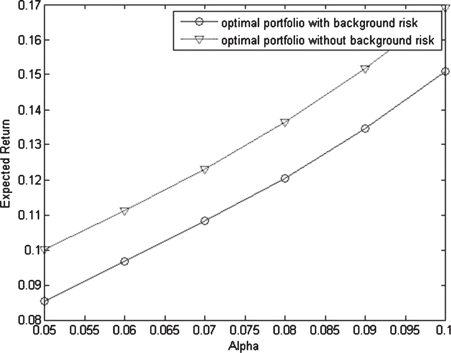
To demonstrate more clearly the difference of optimal portfolios with background risk from those without, we do experiments by keeping the threshold return level at – 8% and changing. The optimal portfolios with or without background risk at different tolerable chance levels are obtained and shown in Tables 2 and 3, respectively.

Through Tables 2, 3 and Fig. 1, we can see the results as follows. (a) When the tolerable level is the same, the expected return of the portfolio with background risk will be lower, and the expected return will increase when the tolerable level increases; (b) The effective frontier without background risk is more than that with background risk; (c) When α = 0.06, 0.1111 > 0.0966, which means in the same situation, the expected return without background risk is larger than that with backgroundrisk.

OPEN IN VIEWER

Fig.1

Optimal portfolios with background risk and without background risk in Tables 2 and 3.

This numerical example is to illustrate our proposed approach for the uncertain portfolio selection with mental accounts. We give a numerical example here. We select twenty stocks from Shanghai Stock Exchange. Normal uncertain distributions of the stock return are shown in Table 1. Suppose the investors have two mental accounts: Savings (50%) and Consumption (50%). The investors choose the same 20 stocks in Table 1.

and

In the savings account, suppose the threshold of the expected return α = 5% , H₁ = -5 %. So the model (25) can be written in this form: { max ∑ i = 1 20 x 1 i μ i s . t . ∑ i = 1 20 x 1 i μ i - 1.6234 ∑ i = 1 20 x 1 i σ i ⩾ - 0.05 , ∑ i = 1 20 x 1 i = 1 , 0 ⩽ x ki ⩽ 0.8 , i = 1 , 2 , ⋯ , n , k = 1 , 2 , ⋯ , m .(34)

In the consumption account, we suppose the threshold of the expected return α = 5% , H₂ = -10 %. So the model (25) can be written in thisform: { max ∑ i = 1 20 x 2 i μ i s . t . ∑ i = 1 20 x 2 i μ i - 1.6234 ∑ i = 1 20 x 2 i σ i ⩾ - 0.10 , ∑ i = 1 20 x 2 i = 1 , 0 ⩽ x ki ⩽ 0.8 , i = 1 , 2 , ⋯ , n , k = 1 , 2 , ⋯ , m .(35)

Using MATLAB, we can get the optimal portfolio of different mental accounts and provide it in Table 4. The optimal solution of the total account is also shown in Table 4. It is obvious that because the risk tolerance level is different, the proportions of stocks of different optimal portfolios of two accounts are not the same. And the expected return of consumption account is higher while the expected return of savings is lower. The expected return of total account is between those two.

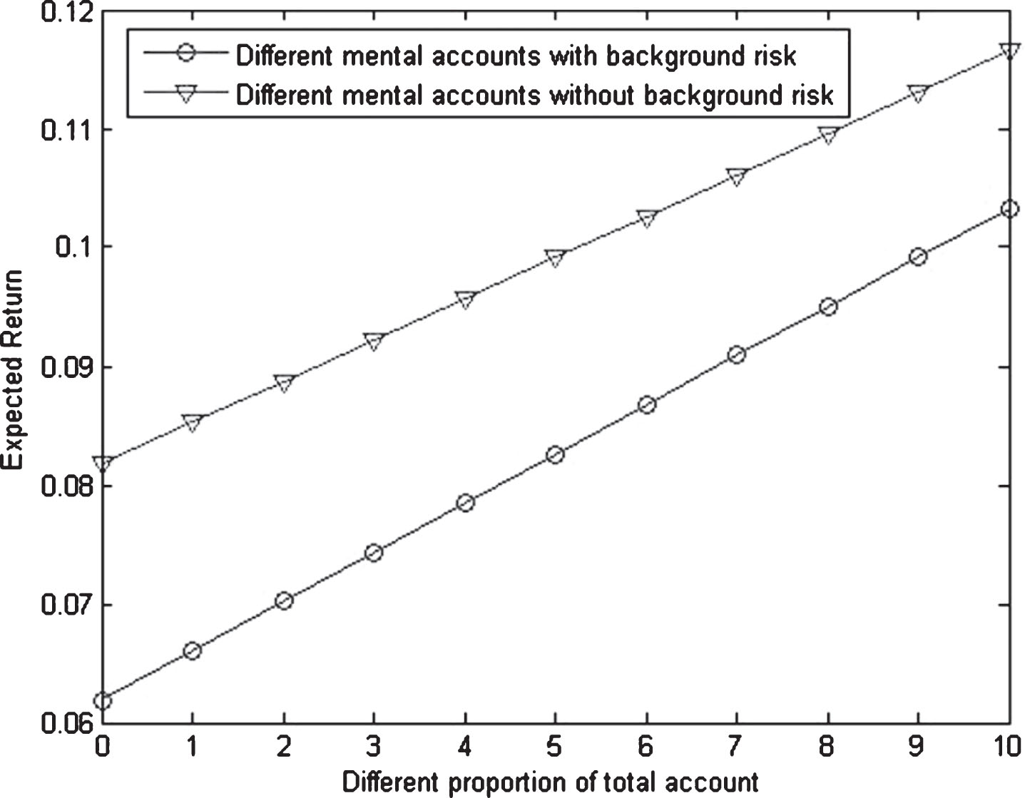
We change the proportion of two accounts from 10 : 0, 9 : 1 to 0 : 10 so that we get the optimal solution and the total expected return. We draw the result in Fig. 2.

OPEN IN VIEWER

Fig.2

Expected return of different total accounts in Table 4.

Figure 2 shows these facts as follows. (a) When the proportion of savings account decreases while that of the consumption account increasing, the total expected return increases; (b) When the proportion of savings to consumption account is 9 : 1, the expected return is 7.36%; when the proportion of savings to consumption account is 5 : 5, the expected return is 9.27%; when the proportion of savings to consumption account is 1 : 9, the expected returnis 11.17%.

We describe the uncertain portfolio considering both the background risk and the mental account model through a numerical example. We suppose that the investor has two mental accounts: savings (50%) and consumption (50%). Assuming that the investor also chooses the same 20 securities as those in Chapter 3, experts considers that the return rate of the background asset has an uncertain distribution function r _b  ∼ N (0, 0.01).

4.3.2 Model for uncertain portfolio of consumption account with background risks

{ max ∑ i = 1 20 x 1 i μ i s . t . ∑ i = 1 20 x 1 i μ i - 1.6234 ∑ i = 1 20 x 1 i σ i ⩾ - 0.06 , ∑ i = 1 20 x 1 i = 1 , 0 ⩽ x i ⩽ 0.8 , i = 1 , 2 , ⋯ , 20 .(37)

Figure 3 shows these results as follows. (a) When the level of tolerance is the same, the expected return of a portfolio that considers background risk is lower than that doesn’t; (b) The result also shows that when the percent of savings account decreases while that of the consumption account increasing, the total expected return increases; (c) When the proportion of savings to consumption is 9 : 1, the expected return is 8.53%; when the proportion of savings to consumption is 5 : 5, the expected return is 9.92%; when the proportion of savings to consumption is 1 : 9, the expected return is 11.30%; (d) the effective frontier without background risk is more efficient than that with background risk.

OPEN IN VIEWER

Fig.3

Expected return of different total accounts in Tables 5and 6.

In the consumption account, investors set the threshold of income α = 5% , H₁ = -10 %. We can also get an uncertain portfolio model that considers background risk and one that does not. By solving the model, we obtain the optimal solution of the uncertain portfolio of background risk and the uncertain portfolio model which does not consider the background risk under different mental accounts, as shown in Tables 5 and 6. Under the savings account, if the background risk is taken into account, the maximum expected return for the investor is 5.96%. If the background risk is not taken into account, the maximum expected return for investors is 8.38% and we can see that 5.96% <8.38 %, which means that the expected return of the sub-portfolio considering background risk is less than the sub-portfolio expected return. In the consumption account, we can get the same conclusion. The optimal solutions of the total portfolio considering and not considering the background risk are also shown in Tables 5 and 6, respectively. We can see that the expected return of the total portfolio considering the background risk is 10.33%, and that without considering the background risk is 11.65%, obviously 10.33% <11.65 %. The expected return is also less than the expected return of the total portfolio without considering the background risk.

OPEN IN VIEWER

Table 5

Optimal portfolio of different mental accounts with background risk in model (35)

Savings: Consumption	Stock 2	Stock 4	Stock 10	Stock 13	Expected return
10 : 0	0.80030	0.00000	0.00000	0.20280	6.19%
9 : 1	0.72027	0.02364	0.07637	0.19129	6.60%
8 : 2	0.64024	0.04728	0.15274	0.17978	7.02%
7 : 3	0.56021	0.07092	0.22911	0.16827	7.43%
6 : 4	0.48018	0.09456	0.30548	0.15676	7.85%
5 : 5	0.40015	0.1182	0.38185	0.14525	8.26%
4 : 6	0.32012	0.14184	0.45822	0.13374	8.67%
3 : 7	0.24009	0.16548	0.53459	0.12223	9.09%
2 : 8	0.16006	0.18912	0.61096	0.11072	9.50%
1 : 9	0.08003	0.21276	0.68733	0.09921	9.92%
0 : 10	0.00000	0.23640	0.76370	0.08770	10.33%

OPEN IN VIEWER

Table 6

Optimal portfolio of different mental accounts without background risk in model (36)

Savings: Consumption	Stock 2	Stock 4	Stock 10	Expected return
10 : 0	0.17060	0.0294	0.80000	8.18%
9 : 1	0.15354	0.0664	0.78006	8.53%
8 : 2	0.13648	0.1034	0.76012	8.87%
7 : 3	0.11942	0.1404	0.74018	9.22%
6 : 4	0.10236	0.1774	0.72024	9.57%
5 : 5	0.0853	0.2144	0.7003	9.92%
4 : 6	0.06824	0.2514	0.68036	10.26%
3 : 7	0.05118	0.2884	0.66042	10.61%
2 : 8	0.03412	0.3254	0.64048	10.96%
1 : 9	0.01706	0.3624	0.62054	11.30%
0 : 10	0.00000	0.3994	0.60060	11.65%