Investor sentiment index based on intuitionistic fuzzy analytic network process method and empirical analysis 1

Abstract

This paper presents a network index system for assessing investor sentiment. The proposed comprehensive investor sentiment index is based on intuitionistic fuzzy analytic network process (IFANP) and regression model, and is compared with a sentiment index constructed on the basis of principal component analysis (PCA). The long-term relationship and dynamic relationship between the yields of these investor sentiment indexes and the Shanghai Composite Index (SHCI) are explored. Based on autoregressive moving average models and cointegration models, short-term and medium-term forecasts of the yields of investor sentiment index and SHCI are derived. The results of cointegration test, short-term forecasting and medium-term forecasting all show that the investor sentiment index based on IFANP is superior to that based on PCA.

Keywords

Intuitionistic fuzzy set intuitionistic fuzzy analytic network process principal component analysis investor sentiment

1 Introduction

Sentiment is a general term for a series of subjective cognitions. It is the psychological and physiological state of a variety of feelings, thoughts, and behaviors. Investor sentiment, which can affect decision making, plays an important role in studies of behavioral finance.

The Bearish Sentiment Index first appeared in the American magazine “Investor Intelligence” in 1963, also describing the concept of investor sentiment for the first time. Since then, scholars have defined investor sentiment from different perspectives. For instance, Zweig developed a theory of investor expectations from the values of the underlying securities [1]. Lee et al. believed that investor sentiment was a kind of market judgment based on investors’ psychological emotions, rooted in the cognitive bias caused by the irrational psychological factors of investors [2]. Brown and Cliff stated that investor sentiment incorporated optimistic or pessimistic expectations about stock prices [3], whereas Baker and Wurgler argued that investor sentiment was not only a certain expectation, but it is also investors’ propensity to speculate [4]. Wurgler pointed out that the past definitions of investor sentiment had only been derived from traditional finance, and their boundaries were not very clear [5]. Bormann explained market sentiment from a psychological perspective [6], while Galariotis et al. pointed out that expectation and sentiment may affect the relationship between momentum and state [7].

Investors receive a lot of information from the stock market every day. Because of different cognitions about the market or different information processing abilities of the investors, different expectations for the stock market are formed. The present paper considers this bullish or bearish expectation to be “investor sentiment.”

Fuzzy set is a powerful tool to deal with the imprecision and vagueness, and it has been widely used in decision-making and evaluation process. For instance, Ali Khan et al. introduced multiattribute group decision-making based on Pythagorean fuzzy set [8], while Shakeel et al. investigated information aggregation methods under Pythagorean trapezoidal fuzzy environment and proposed new multi-attribute group decision making methods under the Pythagorean trapezoidal fuzzy environment [9]. Khan et al. defined some operators for Pythagorean fuzzy sets and interval-valued Pythagorean fuzzy sets and suggested multi-criteria decision-making approach based on the developed operators [10], while Ashraf et al. examined the basic operations of spherical fuzzy sets and developed a multi attribute decision making method [11]. Khan et al. proposed new Pythagorean trapezoidal uncertain linguistic fuzzy aggregation information and studied its properties [12].

This paper focuses on constructing a comprehensive investor sentiment index, which is based on intuitionistic fuzzy analytic network process and regression model. This paper has scientific value for its following contributions.

Compared with other literatures, a new perspective for constructing investor sentiment index is provided. We take into account the interaction and feedback relationships among criteria and indices, and also consider the fuzziness and uncertainty in the evaluation process. This paper presents an application study to demonstrate the effectiveness, applicability and superiority of IFANP in practical application. As far as these authors are able to identify, there is no extant research which combines IFANP with regression model for constructing investor sentiment index. To demonstrate the superiority of the proposed method, we compared it with the sentiment index based on principal component analysis.

2 Literature review

It is difficult to find a unified definition of investor sentiment, because it belongs to the category of behavioral finance and is difficult to observe and measure directly. Scholars usually choose different market variables as proxies for investor sentiment. These variables can be divided into four categories. The first includes subjective indicators of investor sentiment. These are generally obtained through questionnaire surveys and statistical analysis, and can directly reflect whether the investors are optimistic or pessimistic about the future of the market. These indices are subjective and ex ante, such as the Wall Street Analyst Index, Friendship Index, the American Association of Individual Investors, and the Investors Intelligence. Liston developed individual investor sentiment and institutional investor sentiment for different investors [13]. Sun et al. examined the predictability of intraday market return with changes in high-frequency investor sentiment, and their investor sentiment measure was based on the proprietary Thomson Reuters MarketPsych index [14].

The second category covers objective indices of investor sentiment. These indicators can be acquired by applying certain statistical methods to public stock market trading data. These indices are relatively objective and ex post, such as the closed-end funds discount rate, turnover rate, and IPO quantity. Jitmaneeroj argued that the trading volume, advance-decline ratio, and price volatility are strong proxies for market-based sentiment [15]. Ruan et al. investigated the cross-correlation between individual investor sentiment and the Chinese stock market by analyzing the Yu¢ebao Sentiment Index, the daily closing prices of the SHCI and the Shenzhen Component Index [16].

The third category incorporates invisible factors of non-economic variables that affect investor sentiment. For example, these could be weather-related variables such as temperature [17], air pressure, and humidity, or other factors such as noise and sports games [18]. These indicators are not directly relevant to the financial market, and their internal influence mechanisms are difficult to elaborate.

The fourth category is the comprehensive sentiment index, which is constructed from a number of subjective or objective proxy variables. Baker and Wurgler presented a comprehensive investor sentiment index using the net asset values of closed-end stock fund, the raw turnover ratio, the number of IPOs, first-day returns, the share of equity and the dividend premium [19]. With this investor sentiment index, scholars further explored investor sentiment and the stock returns and the role of investor sentiment in the long-term correlation between U.S. stock and bond markets [20]. A comprehensive index has been developed using proxy variables such as the average stock return and average turnover volume [21]. A separate study selected the German Consumer Confidence Index and trading volume as the variables [22].

Investor sentiment is affected by stock prices, which in turn are affected by investor sentiment. Moreover, investor sentiment will increase the volatility and duration of market trends. Through the study of investor sentiment in Britain, the United States, Japan, Germany, France, and Canada, Baker and Stein found that investor sentiment had cross-sectional effects on different types of stock portfolios [23]. Brown and Cliff believed that investor sentiment and the market return index had a negative correlation over the next 1–3 years, arguing that investor sentiment had a certain predictive ability with respect to long-term stock returns [24]. Schmeling stated that the consumer confidence index represented individual investor sentiment, which was negatively correlated with market return [25]. Huang et al. believed that aligned investor sentiments are a powerful predictor of stock returns, outperforming well-recognized macroeconomic variables and predicting cross-sectional stock returns [26]. Sibley et al. showed that the power of the sentiment index to predict cross-sectional stock returns is mainly driven by the risk/business cycle component [27]. Bekaert and Hoerova found the variance premium to contain a substantial amount of information about risk aversion, whereas the credit spread broadly reflects uncertainty, and discussed sentiment indices and financial stress indices on the basis of risk aversion and uncertainty [28]. Xu and Zhou stated that changes in sentiment had a positive impact on future stock returns in the Chinese A-share market, and the predictive power of the sentiment index was most significant for small-sized portfolios [29].

In the current research, when constructing the investor sentiment index, scholars generally adopt mathematical statistical method to make multiple variables synthesize a new variable. The most common method is principal component analysis [4 , 30], and some scholars also adopt kalman filtering method. Although previous studies have presented many factors related to investor sentiment, the interaction and feedback relationships among these factors were not considered. For example, margin trading has an impact on the trading volume, advance decline ratio, and net capital flow, and vice versa. Moreover, when evaluating the importance of the indicators, there are uncertainties and ambiguities caused by differences in experience and cultural background of evaluators. Therefore, a new method for constructing a composite index of investor sentiment should be proposed.

When the relationship between independent and dependent variables was vague, the event was ambiguous, or the problem was complex and complicated, scholars introduced fuzzy regression analysis. Bisserier et al. proposed a revisited approach for possibilistic fuzzy regression methods [31]. Jiang et al. presented a multi-objective evolutionary approach to fuzzy regression analysis to acquire optimal solutions [32]. Chukhrova and Johannssen provided a comprehensive systematic review and bibliography on the topic of fuzzy regression analysis [33].

This paper examines the comprehensive sentiment index. Although previous research introduced many factors related to investor sentiment, the interaction and feedback relationships among these factors were not taken into account. For example, margin trading has an impact on the trading volume, advance decline ratio, and net capital flow, and vice versa. Therefore, the interaction and feedback relationships among criteria and indices must be considered. This paper develops a network structure of the various indicators related to investor sentiment. Moreover, when evaluating the importance of the indicators, there are uncertainties and ambiguities caused by differences in experience and cultural background of evaluators. Consequently, the fuzziness and uncertainty in the evaluation process are considered in this paper, and a comprehensive sentiment index is proposed based on the IFANP.

3 Preliminary knowledge

3.1 Analytic network process

ANP was introduced by Saaty as an extension of the analytic hierarchy process (AHP) [34]. Importantly, ANP considers the interaction and feedback relationships among elements, thus overcoming several limitations of AHP. In ANP, elements are divided into two parts, the control layer and the network layer. The structure of ANP is shown in Fig. 1. Wherein, “Goal” represents the overall objective, and “C₁ ... C_n” represents the criteria in the control layer. “A, B ... N” represents the indicator sets that have interaction and feedback relationships in the network layer. Generally, if the indicator set A has an influence on set B, then an arrow is added from A to B; if there are interaction relationships within the indicator set A, then an arrow is added from A to A.

Fig. 1

A typical ANP structure.

As shown in Fig. 1, the first part is the control layer, which mainly includes the overall objective and criteria. In this part, each criterion is independent and is governed solely by the overall goal. In particular, it is possible to have no criteria in the control layer, but there must be at least one goal. Therefore, the control layer can be regarded as a traditional AHP structure, and the corresponding weights can be acquired by the AHP method.

The second part is the network layer, which consists of all elements that have interaction and feedback relationships. The possible relationships in this layer include the domination of upper elements over lower elements; the interdependence of elements in the same layer; and the feedback of elements in the lower layer to those in the upper layer. The weights can be obtained by constructing an unweighted supermatrix, weighted supermatrix, and limit supermatrix on the basis of the interaction and feedback relationships.

3.2 Intuitionistic fuzzy preference relationship

When comparing the importance of indicators, experts or decision makers need to provide information about their preferences for each indicator. However, because of the fuzziness and uncertainty in the environment and differences in people’s way of thinking, the preference information given by the evaluators generally cannot be expressed by an exact number. A more realistic approach is to use fuzzy values instead of exact numerical values. Atanassov introduced the definition and operation rules of intuitionistic fuzzy sets [35]. In an intuitionistic fuzzy set, each element is assigned a membership degree, a non-membership degree, and a hesitation degree. Dimitrov defined the intuitionistic fuzzy preference relationship (IFPR), a generalization of the fuzzy preference relationship that allows the fuzziness and uncertainty to be described more comprehensively and flexibly [36].

Let X = {x₁, x₂, …, x_n} be evaluation indices. Judgment matrix R is formed by the preference information of the evaluators. The elements in R are represented by intuitionistic fuzzy numbers, denoted as (μij, vij), where μij indicates the degree to which xi is more advantageous than xj; vij indicates the degree to which xi is more disadvantageous than xj; and π_ij = (1 - μ_ij - ν_ij) indicates the degree of hesitancy or uncertainty.

$\begin{matrix} R = (μ_{ij}, ν_{ij}) = \\ (\begin{matrix} (μ_{11}, ν_{11}) & (μ_{12}, ν_{12}) & \dots & (μ_{1 n}, ν_{1 n}) \\ (μ_{21}, ν_{21}) & (μ_{22}, ν_{22}) & \dots & (μ_{2 n}, ν_{2 n}) \\ ⋮ & ⋮ & ⋱ & ⋮ \\ (μ_{n 1}, ν_{n 1}) & (μ_{n 2}, ν_{n 2}) & \dots & (μ_{nn}, ν_{nn}) \end{matrix}) \end{matrix}$ (1) where μ_ij, ν_ij ∈ [0, 1], 0 ≤ μ_ij + ν_ij ≤ 1, μ_ij = ν_ji, u_ii = v_ii = 0.5, i, j = 1, 2, ... , n.

The least-squares and goal programming methods can be applied to determine the local weights of IFPRs. In this paper, the optimal priority optimization (OPO) model is adopted to acquire the local weights [37].

$\begin{matrix} Max τ \end{matrix}$

$s . t {\begin{matrix} 1 - \frac{P_{l} \bar{ϖ}}{t_{l}} \geq τ, l = 1, 2, \dots, m, \\ m = n (n - 1), \\ 0 \leq {\bar{ϖ}}_{i} \leq 1, i = 1, 2, \dots m, \\ \sum_{i = 1}^{n} {\bar{ϖ}}_{i} = 1, \end{matrix}$ (2) where ϖ^* denotes the local weights of IFPRs; P_l is an m×n matrix, and m = n(n–1); t_l indicates the tolerance parameter satisfying matrix consistency; and τ^* denotes the optimal objective function value, which can also be regarded as the consistency index. If τ^* is equal or greater than one, then the IFPR satisfies the consistency requirement; if τ^* is between zero and one, then the IFPR is inconsistent. If the consistency requirement is not satisfied, then Eqs. (16) and (17) in the study by Xu and Liao can be used to improve this value [38].

3.3 Intuitionistic fuzzy and analytic network process

In recent years, considering the fuzziness of ideographic meaning, the study of fuzzy analytic network process (FANP) is very prosperous. FANP is an extension of ANP in uncertainty and fuzziness problems. Mikhailov and Singh proposed a fuzzy extension to the network analysis of Saaty, adding human preference information to the ANP method, and proposing a two-dimensional interval [a, b] to express the uncertainty and fuzziness in the decision-making process [39]. Bueyuekoezkan et al. constructed a fuzzy network analysis method based on triangular fuzzy Numbers, which solved the fuzziness problem in the process of criterion measurement and judgment [40]. Chang et al. proposed to use triangular fuzzy number to represent the preference information of decision makers, and to use expert knowledge system and fuzzy network analysis to solve uncertain or inaccurate evaluation problems [41]. Lin applies FANP method to supplier selection in the supply chain [42].

However, how to apply ANP under intuitionistic fuzzy environment becomes a difficult problem. In the existing studies, the combination of intuitionistic fuzzy set and AHP can be found. For example, Sadiq and Tesfamariam applied IFAHP to handle both vagueness and ambiguity related uncertainties in the environmental decision-making process [43]. Abdullah and Najib proposed a new IFAHP method characterised by new preference scale of pair-wise comparison matrix measurement [44]. Kahraman et al. proposed an interval-valued IFAHP for order of preference by similarity to ideal solution based methodology, and an application is provided for the evaluation of outsource manufacturers [45]. AHP and ANP are different technologies, and IFANP is rarely used in literature. Buyukozkan et al. combined IF with ANP with limited computational steps [46]. Liao et al. combined these two theories and proposed the calculation of intuitionistic fuzzy network analysis for the first time [37]. At present, limited applications of IFANP imply some gaps in the literature.

3.4 Principal component analysis

Principal component analysis is a multivariate statistical method that examines the correlation between multiple variables. It is often used as a method to reveal the internal structure among multiple variables through a few principal components. The main purpose of principal component analysis is to reduce dimensionality. Suppose there are n sentiment indicators, and the initial matrix reflects the p phase observations of these indicators. $X = (X_{1}, X_{2}, \dots, X_{n})^{T} = [\begin{matrix} x_{11} & x_{21} & \dots & x_{n 1} \\ x_{12} & x_{22} & \dots & x_{n 2} \\ ⋮ & ⋮ & ⋱ & ⋮ \\ x_{1 p} & x_{2 p} & \dots & x_{np} \end{matrix}]$ where x_ij denotes the observation value of i in period j, X_i = (x_1i, x_2i, …, x_pi) ^T.

For X₁, X₂, . . . , X_n in the matrix, the following linear combination can be constructed: $\begin{matrix} {\begin{matrix} Z_{1} = a_{11} X_{1} + a_{21} X_{2} + \dots + a_{n 1} X_{n}, \\ Z_{2} = a_{12} X_{1} + a_{22} X_{2} + \dots + a_{n 2} X_{n}, \\ ⋮ \\ Z_{p} = a_{1 p} X_{1} + a_{2 p} X_{2} + \dots + a_{np} X_{n}, \end{matrix} \\ {\begin{matrix} \sum_{j = 1}^{n} a_{ij}^{2} = 1 (i, j = 1, 2, \dots, p), \\ \sum_{j = 1}^{p} a_{ij} a_{kj} = 0 (i \neq k), \end{matrix} \end{matrix}$ (3) where Z₁ denotes the largest variance of the first composite indicator. The larger variance of Z₁, the more information Z₁ contains. If Z₁ is not large enough to represent the information of the original indicators, then we select the second linear combination Z₂. Z₂ indicates the second-largest variance of the second composite indicator in all the linear combinations. By analogy, Z_p denotes the minimum variance among all the linear combinations. Finally, the overall principal component is Z (comprehensive sentiment index). $Z = \sum_{i = 1}^{k} a_{i} Z_{j}, (i = 1, 2, \dots, k; j = 1, 2, \dots, p) .$ (4)

Generally, $\sum_{i = 1}^{k} a_{i} \geq 80 %$ , or there are k characteristic roots greater than one, and k is the number of selected principal components.

A number of scholars have explored the PCA-based sentiment index. For instance, Chen et al. developed a PCA-based investor sentiment with six important economic and market factors [47], and Saka et al. revealed the perceived commonality in default risk among peripheral and core Eurozone sovereigns based on PCA [48]. Ding et al. proposed an investor sentiment index for the Chinese stock market based on PCA and an autoregressive model [49].

4 Investor sentiment index based on IFANP

In this section, we first select investor sentiment indicators and examine their interaction and feedback relationships. Then we establish the investor sentiment index based on IFANP and PCA, respectively.

4.1 Sentiment indicator selection and data processing

Inspired by existing research, 13 objective indices were chosen to construct the investor sentiment index considered in this paper. The main reason for excluding subjective indicators is that subjective variables are obtained through questionnaires, and the timeliness of the survey samples will gradually be weakened by the inherent time delays.

The indicators are divided into four categories: market activity index, profitability index, market performance index, and market expansion index. Each indicator is described in Table 1.

Table 1
Sentiment indicators

First level index Second level index Interpretation

Market activity indicator (U₁) Turnover rate (u₁₁) Reflects the market liquidity. The higher the turnover rate, the more enthusiastic are the market participants.

Balance of financing (u₁₂) When the balance of financing is on the rise, investors have an optimistic attitude towards the stock market, and the overall trading status of securities reflects a prosperous environment, and vice versa.

Trading volume (u₁₃) Reflects the quantity of investors buying and selling stocks. The greater the trading volume, the greater the investors’ acceptance degree.

Interbank rate for seven days (u₁₄) Higher interbank rates and higher short-term capital costs will trigger concerns among investors about the liquidity of the market. For investors, these are bearish signals that will increase fear. On the contrary, bullish signals will increase investor optimism.

Profitability indicator (U₂) P/E ratio (u₂₁) A relatively high price/earnings (P/E) ratio shows that the market has investment enthusiasm, potentially increasing the price of the stock in the short-term and bringing returns to investors.

P/B ratio (u₂₂) A high price/book (P/B) ratio indicates that the growth and profitability of the enterprise are high. Investors can judge the operating status and future development of the enterprise by the P/B rate.

First day premium rate of IPO (u₂₃) When investors are optimistic, their sentiments are relatively stable. In this scenario, issuers and underwriters usually raise the price of the IPO, and more companies will raise funds through IPOs.

Market performance indicator (U₃) Advance decline ratio (u₃₁) The main purpose of this metric is to compare the strength of two sides in the stock market, and it is used to reflect the rise and fall of market sentiment. It helps to judge the general situation of the stock market.

Relative strength index (u₃₂) The relative strength index is the number of stocks that have risen by 3% divided by the number of stocks that have dropped by 3%. This index helps to judge the strengths of the long and short sides of the market.

Net capital inflow (u₃₃) Used to describe the flow of funds. The capital flow is the strength of the index’s rise and fall, reflecting the bearish or bullish attitudes of investors.

Market expansion indicator (U4) Number of IPOs per week (u₄₁) The listing of new shares usually stimulates the investors’ desire to buy, which in turn has an important impact on the yields of new shares.

Proportion of new shares (u₄₂) The proportion of new shares is the number of new shares issued each week divided by the number of corporate bonds issued each week. As shares have higher risks than bonds, the higher this proportion, the more optimistic are investors.

Number of newly opened accounts per week (u₄₃) Changes in this value reflect investors’ willingness to invest and their expectations of the stock market. When the stock market is expected to rise, new investors will pour into the market.

First level index	Second level index	Interpretation
Market activity indicator (U₁)	Turnover rate (u₁₁)	Reflects the market liquidity. The higher the turnover rate, the more enthusiastic are the market participants.
	Balance of financing (u₁₂)	When the balance of financing is on the rise, investors have an optimistic attitude towards the stock market, and the overall trading status of securities reflects a prosperous environment, and vice versa.
	Trading volume (u₁₃)	Reflects the quantity of investors buying and selling stocks. The greater the trading volume, the greater the investors’ acceptance degree.
	Interbank rate for seven days (u₁₄)	Higher interbank rates and higher short-term capital costs will trigger concerns among investors about the liquidity of the market. For investors, these are bearish signals that will increase fear. On the contrary, bullish signals will increase investor optimism.
Profitability indicator (U₂)	P/E ratio (u₂₁)	A relatively high price/earnings (P/E) ratio shows that the market has investment enthusiasm, potentially increasing the price of the stock in the short-term and bringing returns to investors.
	P/B ratio (u₂₂)	A high price/book (P/B) ratio indicates that the growth and profitability of the enterprise are high. Investors can judge the operating status and future development of the enterprise by the P/B rate.
	First day premium rate of IPO (u₂₃)	When investors are optimistic, their sentiments are relatively stable. In this scenario, issuers and underwriters usually raise the price of the IPO, and more companies will raise funds through IPOs.
Market performance indicator (U₃)	Advance decline ratio (u₃₁)	The main purpose of this metric is to compare the strength of two sides in the stock market, and it is used to reflect the rise and fall of market sentiment. It helps to judge the general situation of the stock market.
	Relative strength index (u₃₂)	The relative strength index is the number of stocks that have risen by 3% divided by the number of stocks that have dropped by 3%. This index helps to judge the strengths of the long and short sides of the market.
	Net capital inflow (u₃₃)	Used to describe the flow of funds. The capital flow is the strength of the index’s rise and fall, reflecting the bearish or bullish attitudes of investors.
Market expansion indicator (U4)	Number of IPOs per week (u₄₁)	The listing of new shares usually stimulates the investors’ desire to buy, which in turn has an important impact on the yields of new shares.
	Proportion of new shares (u₄₂)	The proportion of new shares is the number of new shares issued each week divided by the number of corporate bonds issued each week. As shares have higher risks than bonds, the higher this proportion, the more optimistic are investors.
	Number of newly opened accounts per week (u₄₃)	Changes in this value reflect investors’ willingness to invest and their expectations of the stock market. When the stock market is expected to rise, new investors will pour into the market.

Chinese A-share data from May 1, 2015, to December 31, 2017, obtained from the Wind and Reith databases, were used as sample data. For various reasons, there are several missing values from IPOs during the selected period; the relevant data were assigned values of zero. As the measurement units vary for different indicators, Equations (5) and (6) were adopted to standardize the data for the comparison, ensuring the values of all indices were within the range [0, 1].

If indicator i is a cost indicator, $z_{ij} = \frac{x_{i}^{max} - x_{ij}}{x_{i}^{max} - x_{i}^{min}} .$ (5)

If indicator i is a benefit indicator, $z_{ij} = \frac{x_{ij} - x_{i}^{min}}{x_{i}^{max} - x_{i}^{min}},$ (6) where $x_{i}^{max}$ and $x_{i}^{min}$ indicate the maximum and minimum of the index, respectively.

4.2 Investor sentiment index based on IFANP

Based on the interrelationships among indicators, we now describe the ANP network structure. The local weights and global weights of the indices are then determined, and the regression model for obtaining the investor sentiment index is proposed. The steps of establishing the investor sentiment index based on IFANP are shown as Fig. 2. The specific steps are as follows.

Fig. 2

The steps of establishing the investor sentiment index based on IFANP.

Step 1: Build the ANP network structure.

Considering the interaction and feedback relationships among indicators, a network index system of investor sentiment is presented. For example, the turnover rate (u₁₁) influences the trading volume (u₁₃), and vice versa. The balance of financing (u₁₂) interacts with the trading volume (u₁₃), as well as the advance decline ratio (u₃₁), relative strength index (u₃₂), and net capital inflow (u₃₃). The network structure of investor sentiment is shown in Fig. 3.

Fig. 3

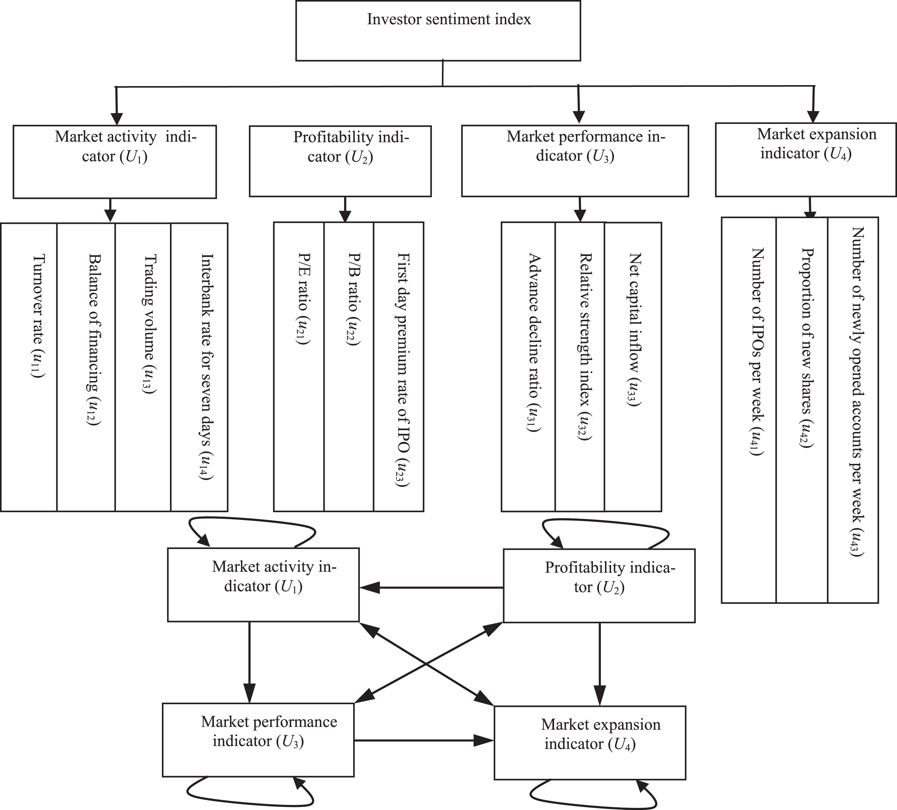
ANP network structure of investor sentiment index.

Step 2: Establish the IFPRs.

People tend to make decisions in a familiar language. For example, the preference for a product can be described by linguistic variables such as like and dislike. IFPRs can express this ambiguity and uncertainty, although linguistic variables can only be used for qualitative analysis. If quantitative analysis or computations are to be performed, the linguistic variables should be converted accordingly. Considering their relative importance, the preference information of evaluators can be divided into nine grades (see Table 2). Note that, according to the actual situation, linguistic variables can also be divided into different levels.

Table 2

Intuitionistic fuzzy linguistic variables

Linguistic variables	Digital scale	Intuitionistic fuzzy value	Hesitation degree
Absolutely unimportant (s₁)	1	(0, 1)	0
Very unimportant (s₂	2	(0.1, 0.8)	0.1
Unimportant s₃)	3	(0.2, 0.6)	0.2
Less unimportant (s₄)	4	(0.35, 0.55)	0.1
Equally important (s₅)	5	(0.5, 0.5)	0
More important (s₆)	6	(0.55, 0.35)	0.1
Important (s₇)	7	(0.6, 0.2)	0.2
Very important (s₈)	8	(0.8, 0.1)	0.1
Absolutely important (s₉)	9	(1, 0)	0

A voting system can be adopted when there are many inconsistent opinions. An intuitional fuzzy number (μ_A, ν_A, π_A) can be obtained by counting the number of votes in support, opposition, and abstention, where μ_A = votes in support / the total number of votes, ν_A = votes in opposition / the total number of votes, and π_A = number of abstentions / the total number of votes.

Under the overall goal, the indicators U₁, U₂, U₃, and U₄ are compared one by one. For instance, compared with U₂, U₃, and U₄, the indicator U₁ is considered relatively important, more important, and very important, respectively. By analogy, a judgment matrix expressed by linguistic variables can be acquired.

According to Table 2, the linguistic variables are converted into corresponding IFPRs, and the following intuitionistic fuzzy judgment matrix is obtained. $R = [\begin{matrix} (0.5, 0.5) (0 . 6, 0 . 2) (0 . 55, 0 . 35) (0 . 8, 0 . 1) \\ (0.2, 0.6) (0 . 5, 0 . 5) (0 . 2, 0 . 6) (0 . 55, 0 . 35) \\ (0.35, 0.55) (0 . 6, 0 . 2) (0 . 5, 0 . 5) (0 . 6, 0 . 2) \\ (0.1, 0.8) (0 . 35, 0 . 55) (0 . 2, 0 . 6) (0 . 5, 0 . 5) \end{matrix}] .$

According to the relationships shown in Fig. 3, a total of 45 IFPR matrices was generated.

Step 3: Construct the unweighted supermatrix.

The local weights of the IFPR matrices were calculated by equation (2). After determining the local weights of all intuitionistic fuzzy judgment matrices, the unweighted supermatrix W is constructed according to Fig. 2 (see Table I in the appendix). $W = [\begin{matrix} W_{11} & W_{12} & \dots & W_{1 N} \\ W_{21} & W_{22} & \dots & W_{2 N} \\ ⋮ & ⋮ & ⋱ & ⋮ \\ W_{N 1} & W_{N 2} & \dots & W_{NN} \end{matrix}] .$

Step 4: Solve the weighted supermatrix.

Only the interaction and feedback relationships among the second-level indicators are considered in the unweighted supermatrix. The global weights of the indices must be calculated. To construct the weighted supermatrix, the weighted matrix a_ij of the relative importance in the first-level indicators is multiplied by the unweighted supermatrix. $\bar{W} = {(a_{ij} \times W)}_{m \times n}, i, j = 1, 2, \dots, n .$ (7)

Step 5: Calculate the limit supermatrix.

To maintain the stability of the weighted supermatrix, its limit can be determined; this is the limit supermatrix. The values of each row in the limit supermatrix are the same, and thus any column can be taken as the global weights of the indicators. The result is presented in Table II in the appendix. $W^{\infty} = lim_{k \to \infty} \frac{1}{N} \sum_{k = 1}^{N} {\bar{W}}^{k} .$

According to Table II, the global weights of the indicators are ω_i = (0.1629, 0.0858, 0.1117, 0.0412, 0.0367, 0.0515, 0.0256, 0.1448, 0.1067, 0.0819, 0.0769, 0.0330, 0.0412) ^T.

Step 6: Acquire the investor sentiment index using a regression model.

The SHCI data from May 1–September 1, 2017, were used to determine the parameters of the investor sentiment index. This period was selected because the data were relatively stable over this time, with relatively little fluctuation, and as this period is relatively recent, the data are representative. Regression and least-squares curve fitting methods are adopted to determine the parameters of the function. $\begin{matrix} fun = x_{1 j} * beta (1) * w (1) + x_{2 j} * beta (2) * w (2) \\ + \dots + x_{ij} * beta (i) * w (i) + \dots + x_{13 j} \\ * beta (13) * w (13) + beta (14), \end{matrix}$ (8) $\begin{matrix} beta & = & lsqcurvefit (fun, beta (), x), \\ x & = & x_{1}, x_{2}, \dots, x_{13}, \end{matrix}$ (9) where x_ij denotes the normalized value of the ith indicator of the jth trading day; w(i) indicates the weight of the ith index; beta(i) denotes the parameter of the ith index; and beta(14) is a constant.

Computations show that [beta(1), beta(2), ... , beta(14)] = [2.22E-14, 2.22E-14, 535.40, -926.78, 16972.13, 3263.53, 2.09E-05, 1.44E-10, 442.25, 410.82, 2.26E-14, 364.17, 2.22E-14, 3049.37].

The investor sentiment index from May 1, 2015, to December 31, 2017, was obtained by Equation (8). A comparison with the SHCI is shown in Fig. 4.

Fig. 4

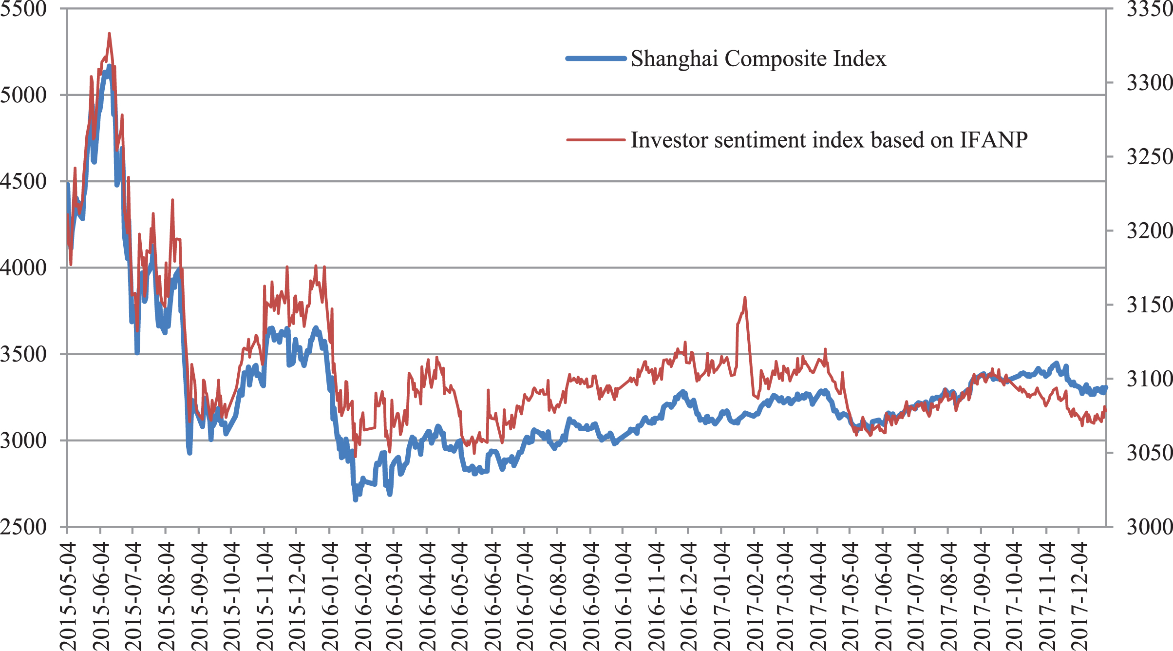
SHCI and investor sentiment index based on IFANP.

In Fig. 4, the trend in the investor sentiment index based on IFANP is basically consistent with that of the SHCI, and there is a significant positive correlation (the correlation coefficient is 0.9157). The investor sentiment index peaked on June 12, 2015, before dropping to around 3175 within one month. During the same period, the SHCI had also dropped rapidly after reaching a high point of 5178.19. Although the investor sentiment index fluctuated during the study period, it has never exceeded the high point of 2015. Correspondingly, the SHCI has also not been able to reach its high point again.

In addition, the investor sentiment index is more sensitive to the stock market than the SHCI. This indicates that the investor sentiment index has a certain reference to the returns on stocks.

4.3 Investor sentiment index based on PCA

Liao et al. implemented the method to a case study concerning the brand management of the six golden flowers of Sichuan liquor to show the applicability and efficiency of the IFANP [33].

To illustrate the scientific nature and superiority of the investor sentiment index based on IFANP, the same data were used to construct an investor sentiment index based on PCA for comparative analysis. The steps of establishing the investor sentiment index based on PCA are shown as Fig. 5. Investor sentiment index based on PCA was constructed as follows.

Fig. 5

The steps of establishing the investor sentiment index based on PCA.

Step 1: Factor analysis was conducted to determine the correlation among indicators, so as to ensure reasonable dimension reduction. The results of the common factor analysis of variance indicate that, except for the trading volume, more than 85% of the information of other variables is retained in the PCA (see Table 3). In Table 3, there are four eigenvalues greater than one, but the cumulative contribution rate is only 71.26%. To raise the cumulative contribution rate above 80%, six principal components were extracted.

Table 3

Total variance of the variables

Component	Initial eigenvalue
	summation	variance %	cumulative %
1	4.3918	33.7830	33.7830
2	2.0789	15.9912	49.7743
3	1.7672	13.5940	63.3683
4	1.0256	7.8892	71.2575
5	0.9605	7.3887	78.6462
6	0.8089	6.2220	84.8682
7	0.6946	5.3431	90.2112
8	0.4610	3.5459	93.7571
9	0.3423	2.6331	96.3902
10	0.1986	1.5279	97.9181
11	0.1724	1.3261	99.2442
12	0.0782	0.6019	99.8461
13	0.0200	0.1539	100.0000

Step 2: Calculate the coefficient matrix. The component matrix is the initial factor load matrix.

Step 3: The function of each principal component is determined as follows.

${\begin{matrix} \begin{matrix} Z_{1} = 0.41 77 * x_{1} + 0.658 0 * x_{2} - 0.30 88 * x_{3} - 0.130 0 * x_{4} + 0.98 88 * x_{5} + 1.023 2 * x_{6} - 0.373 3 * x_{7} \\ + 0.20 59 * x_{8} + 0.28 69 * x_{9} - 0.10 78 * x_{10} - 0.00 49 * x_{11} - 0.472 5 * x_{12} + 5.42 67 * x_{13}, \end{matrix} \\ ⋮ \\ \begin{matrix} Z_{6} = 0.034 4 * x_{1} - 0.00 85 * x_{2} + 0.10 07 * x_{3} + 0.21 47 * x_{4} + 0.00 15 * x_{5} - 0.00 88 * x_{6} + 0.270 2 * x_{7} \\ + 0.266 1 * x_{8} + 0.436 3 * x_{9} - 1.66 39 * x_{10} + 0.083 1 * x_{11} - 0.69 56 * x_{12} - 0.196 4 * x_{13}, \end{matrix} \end{matrix}$ where x₁, x₂, · , x₁₃ are standardized variables and Z₁, Z₂, · , Z₆ denote the principal component functions, respectively.

Step 4: Derive the comprehensive function of the principal components. This is the linear combination of the six principal component functions given by

$\begin{matrix} Z & = & r_{1} * Z_{1} + r_{2} * Z_{2} + r_{3} * Z_{3} + r_{4} * Z_{4} \\ + r_{5} * Z_{5} + r_{6} * Z_{6}, \end{matrix}$ (10) where r₁, r₂, …, r₆ denote the percentage variance of the six principal components, respectively.

The above analysis gives the investor sentiment index based on PCA. A comparison with the SHCI is shown in Fig. 6.

Fig. 6

SHCI and investor sentiment index based on PCA.

According to Fig. 6, the trend of the investor sentiment index based on PCA is basically consistent with that of the SHCI. Although there is a significant positive correlation (the correlation coefficient is 0.8395), it is not as significant as the correlation between SHCI and the investor sentiment index based on IFANP (for which the correlation coefficient is 0.9157).

5 Comparative analysis

Suppose P_t is the closing price of the SHCI on the tth trading day, and H_t and S_t indicate the investor sentiment index values based on IFANP and PCA, respectively. To reduce the heteroscedasticity of the data without changing the trend, the natural logarithm of P_t, H_t, and S_t was taken. The resulting yields are denoted as R_t, I_t, and L_t.

${\begin{matrix} R_{t} = ln (P_{t}) - ln (P_{t - 1}), \\ I_{t} = ln (H_{t}) - ln (H_{t - 1}), \\ L_{t} = ln (S_{t}) - ln (S_{t - 1}) . \end{matrix}$

5.1 Cointegration test

An augmented Dickey–Fuller (ADF) test was performed to check the stationarity of the sequences. The results show that the null hypothesis of unit roots is accepted for P_t, H_t, and S_t, indicating that these sequences are nonstationary. However, the null hypothesis is rejected for R_t, I_t, and L_t, indicating that these are stationary sequences. As R_t, I_t, and L_t are single-integer sequences of the same order, they meet the prerequisites for cointegration analysis. Therefore, the cointegration relationships between R_t and I_t (model 1), R_t and L_t (model 2) were constructed to examine whether any long-term equilibriums exist. The results of the cointegration analysis are presented in Table 4.

Table 4
Results of cointegration analysis

Statistic Cointegration relation

Model 1 Equation R_t₌–0.0002 + 3.8539I_t

T-Statistic (–0.51213) (32.17294)

Prob. (0.0000) (0.0000)

R², F-value 0.720898, 1035.098

Model 2 Equation R_t = –0.0004 + 0.03523L_t

T-Statistic (–0.64814) (8.31525)

Prob. (0.0000) (0.0000)

R², F-value 0.597189, 69.14345

	Statistic	Cointegration relation
Model 1	Equation	R_t₌–0.0002 + 3.8539I_t
	T-Statistic	(–0.51213) (32.17294)
	Prob.	(0.0000) (0.0000)
	R², F-value	0.720898, 1035.098
Model 2	Equation	R_t = –0.0004 + 0.03523L_t
	T-Statistic	(–0.64814) (8.31525)
	Prob.	(0.0000) (0.0000)
	R², F-value	0.597189, 69.14345

In Table 4, the cointegration coefficients of I_t, L_t, and R_t are significant. At the same time, the R values of models 1 and 2 are 0.720898 and 0.597189, respectively. The latter is lower, indicating that the sentiment index based on PCA is not as effective as the sentiment index based on IFANP in terms of model fitness.

Furthermore, stationarity tests were performed on the residuals of the cointegration equations. The results in Table 5 indicate that the residuals are stable, suggesting that there are cointegration relationships between R_t and I_t and between R_t and L_t. In other words, there is a long-term relationship between the yields of the SHCI and the investor sentiment index.

Table 5

Results of ADF tests of the residuals

Sequence	ADF statistic	P-value	Conclusion
resid01	–27.13295	0.0000	stability
resid02	–22.19891	0.0000	stability

5.2 Granger causality test

As there is a cointegration relationship between the yields of the SHCI and the sentiment index, the Granger causality test was applied to examine the causal relationship between them. The results are presented in Table 6.

Table 6
Results of Granger causality tests

Lag order The null hypothesis P-value Conclusion

I_t 1 I_t is not the Granger cause of R_t 0.0300 reject

R_t is not the Granger cause of I_t 0.0156 reject

2 I_t is not the Granger cause of R_t 0.0153 reject

R_t is not the Granger cause of I_t 0.0125 reject

3 I_t is not the Granger cause of R_t 0.0414 reject

R_t is not the Granger cause of I_t 0.0320 reject

L_t 1 L_t is not the Granger cause of R_t 0.2708 accept

R_t is not the Granger cause of L_t 1.E-06 reject

2 L_t is not the Granger cause of R_t 0.2856 accept

R_t is not the Granger cause of L_t 1.E-07 reject

3 L_t is not the Granger cause of R_t 0.4735 accept

R_t is not the Granger cause of L_t 2.E-07 reject

	Lag order	The null hypothesis	P-value	Conclusion
I_t	1	I_t is not the Granger cause of R_t	0.0300	reject
		R_t is not the Granger cause of I_t	0.0156	reject
	2	I_t is not the Granger cause of R_t	0.0153	reject
		R_t is not the Granger cause of I_t	0.0125	reject
	3	I_t is not the Granger cause of R_t	0.0414	reject
		R_t is not the Granger cause of I_t	0.0320	reject
L_t	1	L_t is not the Granger cause of R_t	0.2708	accept
		R_t is not the Granger cause of L_t	1.E-06	reject
	2	L_t is not the Granger cause of R_t	0.2856	accept
		R_t is not the Granger cause of L_t	1.E-07	reject
	3	L_t is not the Granger cause of R_t	0.4735	accept
		R_t is not the Granger cause of L_t	2.E-07	reject

This analysis shows that the Granger causality between R_t and I_t is significant. Regardless of whether the lag order is one, two, or three, I_t is always the Granger cause for the change in R_t, and R_t is the Granger cause for the change in I_t. That is, there is a two-way causality between I_t and R_t. In short, I_t and R_t are an interactive process.

Regardless of the number of lag orders, the causality of L_t to R_t is not significant, whereas that of R_t to L_t is significant. This indicates that there is a one-way causality of the yield of SHCI to the yield of the sentiment index, which is inconsistent with reality.

5.3 Prediction based on the cointegration model

To analyze the degree of fit of I_t / L_t to R_t, an autoregressive moving average (ARMA) model was used to predict I_t and L_t. Short-term and medium-term forecasts for R_t were then generated based on the cointegration model. The fit error rate is given by $p = \sum {(R_{t} f - R_{t})}^{2} / N,$ (11) where p reflects the degree of fit of the model, with smaller values signifying better prediction effects and vice versa. R_tf denotes the predicted yield of the SHCI; R_t denotes the actual yield of the SHCI; and N indicates the total number of observations.

According to the results of the ADF test, I_t and L_t are stationary sequences, and thus the ARMA model can be adopted. As the autocorrelation function (ACF) is trailing off and the partial ACF (PACF) is a second-order truncation, AR(1), AR(2), MA(1), and ARMA(1, 1) for I_t are presented in Table 7.

Table 7

Comparison of different models

Items	AR(1)	AR(2)	MA(1)	ARMA(1, 1)
Constant	–5.61E-05	–5.60E-05	–6.23E-05	–5.38E05
φ ²	–0.1492	–0.1695	–0.1938	0.2181
φ ²		–0.1303		–0.4015
AIC	–8.5362	–8.5489	–8.5397	–8.5446
SIC	–8.5225	–8.5283	–8.5260	–8.5240

$I_{t} = (- 5.60 E - 05) - 0.1695 I_{t - 1} - 0.1303 I_{t - 2} .$ (12)

From Table 7, we find that the Akaike information criterion (AIC) and Schwarz information criterion (SIC) values of model AR(2) are the smallest, which indicates that this model is superior to the others in terms of the model fit. Therefore, model AR(2) is selected. After parameter estimation, the adaptability of the model was tested. Essentially, this is the white noise test of the residual error. If the residual error is not white noise, then some important information has not been extracted, and the model should be reset. The ACF and PACF tests were applied to determine the residual error of model AR(2). The autocorrelation coefficients of the residual error all fell into a random interval, and are significant at the 0.05 confidence level. Therefore, model AR(2) is reasonable, as shown by equation (12). For simplicity, this is named model 3 in the following.

Similarly, ACF and PACF tests were applied to L_t, and models AR(1), AR(2), MA(1), and ARMA(1, 1) were generated. Comparing the AIC and SIC values of these models indicates that ARMA(1, 1) is optimal. As the residual error is white noise, ARMA(1, 1) is a reasonable model, as shown by equation (13). This is referred to as model 4 in the following. $L_{t} = - 0.0020 + 0.6021 L_{t - 1} + ɛ_{t} - 0.8478 ɛ_{t - 1} .$ (13)

5.4 Predictions for different periods

5.4.1 Short-term prediction

The ARMA model was used to predict the yield of the investor sentiment index and the cointegration model was applied to predict the yield of SHCI. The SHCI data from January 1–31, 2018, were used to conduct short-term predictions. Excluding statutory holidays, there were 22 trading days. The results are shown in Fig. 7, where R_tf₁ represents the prediction value based on model 1/3 and R_tf₂ represents the prediction value based on model 2/4.

Fig. 7

Short-term prediction results.

Fig. 7 shows that the trends of the prediction values are in line with the actual values, indicating that the models are effective for short-term predictions. Furthermore, the p-value of the fit error rate of model 1 is 2.55E-05 and that of model 2 is 1.61E-04. The fit error rate of model 1 is obviously lower than that of model 2. This shows that, for short-term forecasting, the sentiment index model based on IFANP is better than that based on PCA.

5.4.2 Medium-term prediction

The SHCI data from January 1–March 31, 2018, were used to make medium-term predictions. Excluding statutory holidays, there was a total of 58 trading days. Dynamic predictions were generated based on model 1/3 and model 2/4, respectively. The results are shown in Fig. 8, where R_tf₃ represents the prediction values based on model 1/3 and R_tf₄ represents the prediction values based on model 2/4.

Fig. 8

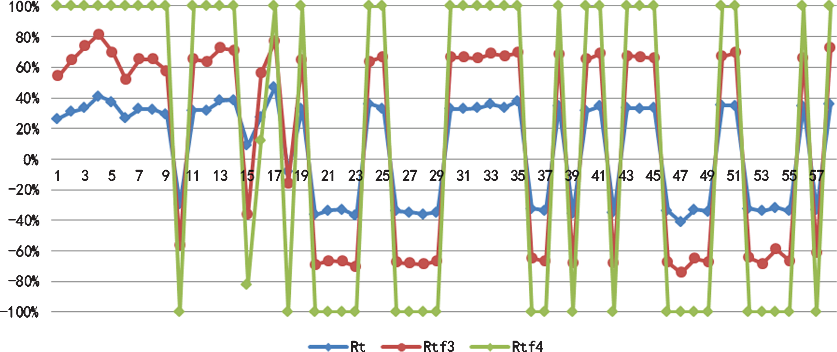
Medium-term prediction results.

Figure 8 shows that the trends of the predicted values are in line with the actual values, indicating that the models are effective for medium-term predictions. Furthermore, the p-value of the fit error rate of model 1 is 1.03E-05, and that of model 2 is 4.85E-04. The fit error rate of model 1 is again less than that of model 2. This shows that, for medium-term forecasting, the sentiment index model based on IFANP is better than the model based on PCA.

Compared with the short-term predictions, the fit error of the medium-term forecasts is obviously lower. The fit error rate of model 1 has decreased from 2.55E-05 to 1.03E-05, and that of model 2 has decreased from 1.6E-04 to 4.85E-05, indicating that the medium-term predictions based on these models are better than the short-term predictions.

6 Conclusions

Objective indicators of market trading were used to construct investor sentiment indexes based on IFANP and PCA, respectively, and the relationship between these indexes and SHCI was analyzed. On the basis of the yields of the investor sentiment indexes and SHCI, the long-term equilibria and dynamic relationships were examined. Short-term and medium-term forecasts of the rate of return were then generated. The main conclusions are as follows.

The cointegration test shows that there is a long-term equilibrium relationship between the yield of the investor sentiment index and the yield of the SHCI. The degree of fit of the investor sentiment index based on IFANP is better than that based on PCA.

According to the Granger causality test, there is a two-way causality between the yield of the investor sentiment index based on IFANP and the yield of the SHCI. The investor sentiment and the stock market are a mutual promotion process. In contrast, there is a one-way causality of the yield of the SHCI to the return from the sentiment index based on PCA, which is inconsistent with reality.

The total weight of four indicators (turnover rate, trading volume, advance decline ratio, relative strength index) is 0.5261. These account for more than half of all the 13 sentiment indicators. Therefore, if it is necessary to regulate the stock market, regulators should focus on these four indicators.

Based on the ARMA model and the cointegration model, short-term and medium-term forecasts of the yields of the investor sentiment index and SHCI were generated. The medium-term predictions are better than the short-term predictions. Moreover, whether in the short-term or medium-term, the results of the investor sentiment index based on IFANP are superior to those of the sentiment index based on PCA.

General time series methods are based on accurate information and there are definite functional relations between the past, present and future values of time series and white noise. However, the intrinsic behaviors and decision-making characteristics of investors are not clear in financial markets. At the same time, people’s judgments of the past can be ambiguous, and incomplete historical data are abundant. Therefore, in the future research, we will try to introduce fuzzy thinking into the prediction of financial series and establish the prediction model of intuitionistic fuzzy time series. From the perspective of investor sentiment, intuitionistic fuzzy analytic network process can be further used to study the pricing and forecasting of risky assets.

Footnotes

Appendix

Table 1

The unweighted supermatrix

u ₁₁	u ₁₂	u ₁₃	u ₁₄	u ₂₁	u ₂₂	u ₂₃	u ₃₁	u ₃₂	u ₃₃	u ₄₁	u ₄₂	u ₄₃
u ₁₁	0.0000	0.6618	0.8068	0.4578	0.2395	0.2338	0.4673	0.0000	0.0000	0.0000	0.5133	0.1407	0.4716
u ₁₂	0.2593	0.0000	0.1594	0.2169	0.3605	0.4293	0.1611	0.0000	0.0000	0.0000	0.1773	0.5760	0.1529
u ₁₃	0.6296	0.3043	0.0000	0.3253	0.2395	0.2226	0.2683	0.0000	0.0000	0.0000	0.0932	0.1511	0.2735
u ₁₄	0.1111	0.0338	0.0338	0.0000	0.1606	0.1143	0.1033	0.0000	0.0000	0.0000	0.2162	0.1322	0.1020
u ₂₁	0.0000	0.0000	0.0000	0.0000	0.0000	0.8500	0.6000	0.3253	0.3253	0.2105	0.0000	0.0000	0.0000
u ₂₂	0.0000	0.0000	0.0000	0.0000	0.6000	0.0000	0.4000	0.2169	0.2169	0.1403	0.0000	0.0000	0.0000
u ₂₃	0.0000	0.0000	0.0000	0.0000	0.4000	0.1500	0.0000	0.4578	0.4578	0.6491	0.0000	0.0000	0.0000
u ₃₁	0.5601	0.3012	0.4578	0.5601	0.2105	0.2921	0.4578	0.0000	0.8500	0.6000	0.0000	0.0000	0.0000
u ₃₂	0.2921	0.2452	0.3253	0.2921	0.1403	0.1478	0.3253	0.6000	0.0000	0.4000	0.0000	0.0000	0.0000
u ₃₃	0.1478	0.4535	0.2169	0.1478	0.6491	0.5601	0.2169	0.4000	0.1500	0.0000	0.0000	0.0000	0.0000
u ₄₁	0.5601	0.4578	0.4578	0.5601	0.5601	0.5601	0.4578	0.4578	0.4578	0.5601	0.4000	0.6000	0.8500
u ₄₂	0.1478	0.2169	0.2169	0.1478	0.1478	0.1478	0.2169	0.2169	0.2169	0.1478	0.6000	0.0000	0.1500
u ₄₃	0.2921	0.3253	0.3253	0.2921	0.2921	0.2921	0.3253	0.3253	0.3253	0.2921	0.0000	0.4000	0.0000

Table 2

The limit supermatrix

	u ₁₁	u ₁₂	u ₁₃	u ₁₄	u ₂₁	u ₂₂	u ₂₃	u ₃₁	u ₃₂	u ₃₃	u ₄₁	u ₄₂	u ₄₃
u ₁₁	0.1629	0.1629	0.1629	0.1629	0.1629	0.1629	0.1629	0.1629	0.1629	0.1629	0.1629	0.1629	0.1629
u ₁₂	0.0858	0.0858	0.0858	0.0858	0.0858	0.0858	0.0858	0.0858	0.0858	0.0858	0.0858	0.0858	0.0858
u ₁₃	0.1117	0.1117	0.1117	0.1117	0.1117	0.1117	0.1117	0.1117	0.1117	0.1117	0.1117	0.1117	0.1117
u ₁₄	0.0412	0.0412	0.0412	0.0412	0.0412	0.0412	0.0412	0.0412	0.0412	0.0412	0.0412	0.0412	0.0412
u ₂₁	0.0367	0.0367	0.0367	0.0367	0.0367	0.0367	0.0367	0.0367	0.0367	0.0367	0.0367	0.0367	0.0367
u ₂₂	0.0515	0.0515	0.0515	0.0515	0.0515	0.0515	0.0515	0.0515	0.0515	0.0515	0.0515	0.0515	0.0515
u ₂₃	0.0256	0.0256	0.0256	0.0256	0.0256	0.0256	0.0256	0.0256	0.0256	0.0256	0.0256	0.0256	0.0256
u ₃₁	0.1448	0.1448	0.1448	0.1448	0.1448	0.1448	0.1448	0.1448	0.1448	0.1448	0.1448	0.1448	0.1448
u ₃₂	0.1067	0.1067	0.1067	0.1067	0.1067	0.1067	0.1067	0.1067	0.1067	0.1067	0.1067	0.1067	0.1067
u ₃₃	0.0819	0.0819	0.0819	0.0819	0.0819	0.0819	0.0819	0.0819	0.0819	0.0819	0.0819	0.0819	0.0819
u ₄₁	0.0769	0.0769	0.0769	0.0769	0.0769	0.0769	0.0769	0.0769	0.0769	0.0769	0.0769	0.0769	0.0769
u ₄₂	0.0330	0.0330	0.0330	0.0330	0.0330	0.0330	0.0330	0.0330	0.0330	0.0330	0.0330	0.0330	0.0330
u ₄₃	0.0412	0.0412	0.0412	0.0412	0.0412	0.0412	0.0412	0.0412	0.0412	0.0412	0.0412	0.0412	0.0412

References

Zweig

M.E.

, An investor expectations stock price predictive model using closedend fund premiums, The Journal of Finance 28(1) (1973), 67–78.

Lee

C.M.C.

, Shleifer

and Thaler

R.H.

, Investor Sentiment and the Closed-End Fund Puzzle, Journal of Finance 46(1) (1991), 75–109.

Brown

G.W.

and Cliff

M.T.

, Investor sentiment and the near-term stock market, Journal of Empirical Finance 11(1) (2004), 1–27.

Baker

and Wurgler

, Investor Sentiment and the Cross-Section of Stock Returns, The Journal of Finance 61(4) (2006), 1645–1680.

Wurgler

, Introduction: A special issue on investor sentiment, Journal of Financial Economics 104(2) (2012), 227–227.

Bormann

S.K.

, Sentiment indices on financial markets: What do they measure? Economics Discussion Papers 58 (2013), 1–41.

Galariotis

E.C.

, Holmes

, Kallinterakis

and Ma

X.S.

, Market states, expectations, sentiment and momentum: how naive are investors?, International Review of Financial Analysis 32(3) (2014), 1–12.

Khan

M.S.Ali.

, Abdullah

and Ali

, Multiattribute group decision-making based on Pythagorean fuzzy Einstein prioritized aggregation operators, International Journal of Entelligent Systems 34(5) (2019), 1001–1033.

Shakeel

, Abduulah

, Shahzad

, Mahmood

and Siddiqui

, Averaging aggregation operators with pythagorean trapezoidal fuzzy numbers and their application to group decision making, Journal of Intelligent & Fuzzy Systems 36(2) (2019), 1899–1915.

10.

Khan

A.A.

, Abdullah

, Shakeel

, Khan

and Luo

, A New Ranking Methodology for Pythagorean Trapezoidal Uncertain Linguistic Fuzzy Sets Based on Einstein Operations, Symmetry 11(3) (2019a), 440–469.

11.

Ashraf

, Abdullah

, Mahmood

, Ghani

and Mahmood

, Spherical Fuzzy Sets and Their Applications in Multi-Attribute Decision Making Problems, Journal of Intelligent & Fuzzy Systems 36(3) (2019), 2829–2844.

12.

Khan

, Khan

M.S.A.

, Shahzad

and Abdullah

, Pythagorean cubic fuzzy aggregation operators and their application to multicriteria decision making problems, Journal of Intelligent & Fuzzy Systems 36(1) (2019b), 595–607.

13.

Liston

D.P.

, Sin stock returns and investor sentiment, Quarterly Review of Economics & Finance 59 (2016), 63–70.

14.

Sun

, Najand

and Shen

, Stock return predictability and investor sentiment: A high-frequency perspective, Journal of Banking & Finance 73 (2016), 147–164.

15.

Jitmaneeroj

, Does investor sentiment affect priceearnings ratios? Studies in Economics & Finance 34(2) (2017), 229–237.

16.

Ruan

, Yang

, Lv

and Zhang

, Cross correlations between individual investor sentiment and Chinese stock market return: New perspective based on MFDCCA, Physica A: Statistical Mechanics and Its Applications 503 (2018), 243–256.

17.

Cao

and Wei

, Stock market returns: A note on temperature anomaly, Journal of Banking & Finance 29(6) (2005), 1559–1573.

18.

Edmans

, Garcia

and Norli

Ø.

, Sports Sentiment and Stock Returns, The Journal of Finance 62(4) (2007), 1967–1998.

19.

Aissia

D.B.

, Home and foreign investor sentiment and the stock returns, The Quarterly Review of Economics and Finance 59 (2016), 71–77.

20.

Fang

, Yu

and Huang

, The role of investor sentiment in the long-term correlation between U.S. stock and bond markets, International Review of Economics & Finance 58 (2018), 127–139.

21.

Liao

T.L.

, Huang

C.J.

and Wu

C.Y.

, Do fund managers herd to counter investor sentiment, Journal of Business Research 64(2) (2011), 207–212.

22.

Finter

, Niessen-Ruenzi

J.P.D.A.

and Ruenzi

, The impact of investor sentiment on the German stock market, Zeitschrift Für Betriebswirtschaft 82(2) (2012), 133–163.

23.

Baker

and Stein

J.C.

, Market liquidity as a sentiment indicator, Journal of Financial Markets 7(3) (2004), 271–299.

24.

Brown

G.W.

and Cliff

M.T.

, Investor Sentiment and Asset Valuation, Journal of Business 78(2) (2005), 405–440.

25.

Schmeling

, Investor sentiment and stock returns: Some international evidence, Journal of Empirical Finance 16(3) (2009), 394–408.

26.

Huang

, Jiang

, Tu

and Zhou

, Investor Sentiment Aligned: A Powerful Predictor of Stock Returns, The Review of Financial Studies 28(3) (2015), 791–837.

27.

Sibley

S.E.

, Wang

, Xing

and Zhang

, The information content of the sentiment index, Social Science Electronic Publishing 62 (2016), 164–179.

28.

Bekaert

and Hoerova

, What Do Asset Prices Have to Say About Risk Appetite and Uncertainty? Journal of Banking & Finance 67 (2016), 103–118.

29.

H.C.

and Zhou

W.X.

, A weekly sentiment index and the cross-section of stock returns, Finance Research Letters 27 (2018), 135–139.

30.

and Hung

C.H.

, Investor sentiment as conditioning information in asset pricing, Journal of Banking & Finance 33(5) (2009), 892–903.

31.

Bisserier

, Boukezzoula

and Galichet

, A revisited approach to linear fuzzy regression using trapezoidal fuzzy intervals, Information Sciences 180(19) (2010), 3653–3673.

32.

Jiang

, Kwong

C.K.

, Chan

C.Y.

and Yung

K.L.

, A multi-objective evolutionary approach for fuzzy regression analysis, Expert Systems with Application 130 (2019), 225–235.

33.

Chukhrova

and Johannssen

, Fuzzy regression analysis: Systematic review and bibliography, Applied Soft Computing 84 (2019), 1–29.

34.

Saaty

T.L.

and Saaty

T.L.

, Decision Making with Dependence and Feedback: The Analytic Network Process, International 95(2) (1996), 129–157.

35.

Atanassov

K.T.

, Intuitionistic fuzzy sets, Fuzzy Sets & Systems 20(1) (1986), 87–96.

36.

Dimitrov

, The Paretian liberal with intuitionistic fuzzy preferences: A result, Social Choice and Welfare 23(1) (2004), 149–156.

37.

Liao

, Mi

, Xu

and Herrera

, Intuitionistic Fuzzy Analytic Network Process, IEEE Transactions on Fuzzy Systems 26(5) (2018), 2578–2590.

38.

and Liao

, Intuitionistic Fuzzy Analytic Hierarchy Process, IEEE Transactions on Fuzzy Systems 22(4) (2014), 749–761.

39.

Mikhailov

and Singh

M.G.

, Fuzzy analytic network process and its application to the development of decision support systems, Systems Man & Cybernetics Part C Applications & Reviews IEEE Transactions on 33(1) (2003), 33–41.

40.

Bueyuekoezkan

, Ertay

, Kahraman

and Da

, Determining the Importance Weights for the Design Requirements in the House of Quality Using the Fuzzy Analytic Network Approach, International Journal of Intelligent Systems 19(5) (2004), 443–461.

41.

Chang

C.W.

, Horng

D.J.

and Lin

H.L.

, A measurement model for experts knowledge-based systems algorithm using fuzzy analytic network process, Expert Systems with Applications 38(10) (2011), 12009–12017.

42.

Lin

, An integrated model for supplier selection under a fuzzy situation, International Journal of Production Economics 138(1) (2012), 55–61.

43.

Sadiq

and Tesfamariam

, Environmental decision-making under uncertainty using intuitionistic fuzzy analytic hierarchy process (IF-AHP), Stochastic Environmental Research & Risk Assessment 23(1) (2009), 75–91.

44.

Abdullah

and Najib

, A new preference scale of intuitionistic fuzzy analytic hierarchy process in multi-criteria decision making problems, Journal of Intelligent & Fuzzy Systems 26(2) (2014), 1039–1049.

45.

Kahraman

, Öztayşi

and Onar

S.Ç.

, An integrated intuitionistic fuzzy ahp and topsis approach to evaluation of outsource manufacturers, Journal of Intelligent Systems 29(1) (2020), 283–297.

46.

Buyukozkan

, Guleryuz

and Karpak

, A new combined IF-DEMATEL and IF-ANP approach for CRM partner evaluation, International Journal of Production Economics 191 (2017), 194–206.

47.

Chen

, Chong

T.T.

and Duan

, A principal-component approach to measuring investor sentiment, Quantitative Finance 10(4) (2010), 339–347.

48.

Saka

, Fuertes

A.M.

and Kalotychou

, ECB Policy and Eurozone Fragility: Was De Grauwe Right? Journal of International Money and Finance 54 (2015), 168–185.

49.

Ding

, Liu

, Zhang

and Long

, The contagion effect of international crude oil price fluctuations on Chinese stock market investor sentiment, Applied Energy 187 (2017), 27–36.