Monitoring the process mean using a synthetic X ¯ control chart with two sampling intervals

Abstract

The traditional fixed sampling interval (FSI) synthetic $\bar{X}$ control chart is sensitive to large and moderate process shifts, but insensitive to small process shifts. This paper proposes an improved variable sampling interval (VSI) synthetic $\bar{X}$ control chart with two sampling interval lengths for monitoring the process mean. A Markov chain method is used to compute the adjusted average time to signal (AATS) of the proposed chart. The statistical design of the VSI chart is then formulated and solved with a specific genetic algorithm. Comparisons are made to show the capability of the VSI chart in yielding average performance boost of 16.4%, in the AATS of the VSI chart scheme compared to the situation in which the corresponding FSI chart is used.

Keywords

Statistical process control variable sampling interval adjusted average time to signal

1 Introduction

Faced with fierce competition in today’s global marketplace, for a manufacturing enterprise, quality of production is one of the key factors for the success. Statistical process control (SPC) is a significant method of quality control in which statistical methods are employed to monitor processes and ensure quality. In SPC, control chart is nowadays well established graphical and statistical tool which adopts random sampling to test, record, monitor and assess the quality characteristics of interest gathered from intelligent manufacturing process to detect if the process is under control (Yen et al. [29]). In intelligent manufacturing monitoring, combining the control-chart scheme with other intelligent methods to make the original monitoring methods more efficient has attracted much attention. Such works can be seen in Han et al. [10], He et al. [12], Zhou et al. [34], and many more. Undoubtedly, a more sensitive control chart for the diagnosis of process shift can improve the detection capacity of the integration scheme. For this reason, the improvement of control chart remains a heated topic due to the search for precise methods of quality control.

Since the first control chart, that is, $\bar{X}$ control chart, was developed by Dr. Shewhart in 1924, lots of modifications have been studied to increase the detection power and robustness of control charts. Among these ones, the synthetic $\bar{X}$ control chart introduced by Wu and Spedding [27] is used to detect changes in the process mean. Wu and Spedding [27] declared that the synthetic $\bar{X}$ control chart outperformed the $\bar{X}$ control chart for all levels of shifts in the process mean and the exponentionally weighted moving average (EWMA) and joint $\bar{X}$ -EWMA control charts when the standardized mean shift is lager than 0.8. Inspired by the work of Wu and Spedding [27], numerous studies have been done on synthetic control charts. The most recent research can be seen in Calzada and Scariano [3], Dargopatil and Ghute [8], Lee and Khoo[17], Tran et al. [24], Fang et al. [28], Yeong et al. [30], and many more.

However, the above-mentioned control charts all dealt with the fixed sampling interval (FSI) strategy. The approach to sampling for these control charts is to take samples from the process by using a fixed time interval between samples, and the control charts using this approach are usually called FSI control charts. As we know, to obtain a fast detection of process shifts is one of the main objectives of using control charts, so that the nonconformities can be produced as few as possible before the process shifts are eliminated. In order to utilize the inspection capacity more effectively for better process control, researchers put forward the concept of adaptive control charts in which at least one of design parameters (sampling interval h, sample size n and control limits coefficient k) is allowed to be changed based on the current state of the process. Generally, these adaptive control charts can be categorized into four types: variable sampling interval (VSI) control charts, variable sample size (VSS) control charts, variable control limits (VCL) control charts, and joint-adaptive control charts in which at least two of the design parameters can be changed simultaneously [33]. In general, the VSI scheme is used most often and also the most useful one due to its simplicity and good usability.

The basic idea of using the VSI scheme is: if the current sample indicates a potential shift in the process, the sampling interval before the next sample should be relatively short; but the sampling interval before the next sample should be relatively long if the current sample does not show a process change. When concerning the detection of process shifts, due to using a higher sampling frequency when some indication of a process shift is showed by a sample statistic, VSI control charts are always superior to the corresponding FSI control charts. Nguyen et al.[20] and Safe et al. [22] pointed out that, in long-run context, VSI control charts outperformed VSS and fixed ratio interval control charts for moderate to large process shifts. An extensive amount of works on VSI control charts has been done to improve the charts’ sensitivity for fast detection of process shifts. The most recent research on VSI control charts can be seen in Aslam and Khan [1], [11], Shirke and Barale [23], and so forth. However, we found that although there are some research indicating the benefit of using VSI strategy for $\bar{X}$ control charts, there is still no much research on its impact on the synthetic control chart. Therefore, the aim of this paper is to propose a VSI synthetic $\bar{X}$ control chart for improving the sensitivity of detection of the FSI synthetic chart for slightly process mean shift.

On the other hand, the development of control charts usually assumes the process parameters are known. However, the process parameters are generally unknown in practice. Often the process parameters are estimated by using an in-control historical data set which is collected from Phase I. Undoubtedly, due to the randomness and variability of the estimators adopted during Phase I, the performance of control charts with estimated parameters must be different from the known parameters case. Yeong et al. [30] concluded that regardless of parameter estimates in the design of control charts results in an increase in false alarm rate and an decrease in the ability of control charts to detect the process shifts. Therefore, it is important to discuss the optimal design of control charts in the case where the process parameters are estimated. Many scholars have concerned about this topic, and an early literature review on this topic is given by Jensen et al. [13]. More recently, Cheng and Wang [7], Khoo et al. [14], Mehmood et al. [19] and Zhang et al. [32] studied the optimal design of $\bar{X}$ -type control charts with estimated process parameters. Castagliola et al. [5], Chen [6] and Maravelakis et al. [18] considered the optimal design of dispersion-type control charts with estimated process parameters. In particular, Zhang et al. [31] investigated the performance of the run length of the FSI synthetic $\bar{X}$ control chart with estimated parameters; Yeong et al. [30] studied the effects of process parameters estimation on the cost of the FSI synthetic $\bar{X}$ control chart. In view of the importance of discussing the optimal design of control chart in the estimated process parameters case, this paper investigates the performance of the adjusted average time to signal (AATS) of the proposed VSI synthetic $\bar{X}$ control chart with estimated process parameters. Table 1 provides a summarization of the properties of the existing researches in the literature.

Table 1
Summarized literature review

Papers Type of control chart Type of sampling interval Design method of control chart Type of process parameters

Synthetic chart Others FSI VSI Statistical Economic-statistical Known Estimated

Wu and Spedding (2009) $\sqrt | \bar{X} & CRL$ √ √ √

Calzada et al. (2013) √|CV & CRL √ √ √

Dargopatil and Ghute (2019) √|T² & CRL √ √ √

Lee and Khoo (2019) $\sqrt | DS \bar{X} & CRL$ √ √ √

Lee et al. (2015) $\sqrt | \bar{X} & CRL$ √ √ √

Tran et al. (2019) √|Median chart & CRL √ √ √

Yen et al. (2013) √|TBE & CRL √ √ √

Nguyen et al. (2019) √ √ √ √

Safe et al. (2018) √ √ √ √

Aslam and Khan (2019) √ √ √ √

Haq (2019) √ √ √ √

Shirke and Barale (2019) √ √ √ √

Yeong et al. (2015) $\sqrt | \bar{X} & CRL$ √ √ √

Cheng and Wang (2018) √ √ √ √

Khoo et al. (2013) √ √ √ √

Mehmood et al. (2018) √ √ √ √

Zhang et al. (2012) √ √ √ √

Castagliola et al. (2009) √ √ √ √

Chen (1998) √ √ √ √

Maravelakis et al. (2002) √ √ √ √

Zhang et al. (2011) $\sqrt | \bar{X} & CRL$ √ √ √

The proposed paper $\sqrt | \bar{X} & CRL$ √ √ √

In this paper, consider a process containing a single quality characteristic of interest (denoted by X) following a normal distribution with known mean μ and variance σ², i.e. X ∼ N (μ, σ²). When the process is in control, μ = μ₀ and σ = σ₀. When the process is in an out-of-control state, the process mean changes from μ = μ₀ to μ = μ₀ + δσ₀ (δ is the shift size coefficient) but the value of σ remains unchanged. Assuming that only the occurrence of assignable cause can result in the process mean shift. Additionally, the main objective of this paper is to detect the unilateral process mean shifts, therefore, all expressions are developed hereafter for the case δ ≥ 0.

This article is organized as follows. Section 2 gives an introduction of the FSI synthetic $\bar{X}$ chart. In section 3, the VSI synthetic $\bar{X}$ is proposed and some performance metrics of the chart are calculated. Section 4 rebuilds the VSI chart model under the assumption of estimated parameters. Section 5 develops the statistical design model of VSI synthetic $\bar{X}$ control chart, and a genetic algorithm is developed to solve the model. In Section 6, the AATS performance of the VSI synthetic $\bar{X}$ control chart is compared for the known-parameter and estimated-parameter cases. Finally, Section 7 summarizes the main conclusion.

2 The FSI synthetic

\bar{X}

control chart

The FSI synthetic $\bar{X}$ control chart shown in Figure 1 consists of two control charts: a $\bar{X}$ sub-chart and a CRL sub-chart. The $\bar{X}$ sub-chart consists of three parallel lines, i.e. the lower control limit (LCL), center line (CL) and upper control limit (UCL). The CL represents the target value of the process mean. Unlike in the traditional $\bar{X}$ chart, the synthetic $\bar{X}$ chart does not send an out-of-control signal if a sample mean, $\bar{X}$ , is larger than the UCL of the $\bar{X}$ sub-chart or smaller than the LCL of the $\bar{X}$ sub-chart. In-stead, it just marks a nonconforming sample. The CRL value in using a CRL sub-chart can be defined as the number of $\bar{X}$ samples between the current and the last non-conforming samples. As shown in Figure 1, the white dots represent conforming samples while the black pentagrams represent non-conforming samples in a process. The process starts at t = 0, and three samples of CRL are shown with CRL₁ = 5, CRL₂ = 8, and CRL₃ = 5.

Fig. 1

The FSI synthetic $\bar{X}$ chart.

The steps for developing and implementing the FSI synthetic $\bar{X}$ control chart are as follows:

Decide the LCL and UCL of the $\bar{X}$ sub-chart and the lower control limit, L, of the CRL sub-chart. LCL and UCL can be given by $LCL = μ_{0} - k σ_{\bar{X}},$ (1) $UCL = μ_{0} + k σ_{\bar{X}},$ (2) where $σ_{\bar{X}} = \frac{σ_{0}}{\sqrt{n}}$ , n is the sample size, and k is the control limit coefficient.

At every time interval of h hours, take a random sample of size n and calculate the mean $\bar{X}$ of the sample.

If $LCL \leq \bar{X} \leq UCL$ , the sample is sentenced as conforming and the control flow returns to Step (2).

If $\bar{X} < LCL$ or $\bar{X} > UCL$ , the sample is considered as a non-conforming sample and the control flow goes to Step (3).

The number of $\bar{X}$ samples between two consecutive non-conforming samples is checked. This number is regarded as the CRL value in the synthetic $\bar{X}$ chart.

If CRL ≥ L, the process is still considered as in-control and the control flow returns to Step (2).

If CRL < L, the synthetic chart produces an out-of-control signal and the control flow goes to Step (4).

An investigation is executed to find and eliminate the assignable cause. Then go back to Step (2).

In Wu and Spedding [27]’s work, the optimal values of the design parameters, such as h, n, L and k, are chosen so as to minimize the out-of-control average run length (denoted as ARL₁), with the requirement that must attain an in-control average run length (denoted as ARL₀) equals to a pre-specified value.

The average run length (ARL) of the synthetic $\bar{X}$ control chart is the average number of samples obtained from the start of the process to when the control chart gives an out-of-control signal. ARL is usually studied in two aspects: the in-control ARL (ARL₀) and the out-of-control ARL (ARL₁). ARL₀ is used to measure the false alarm rate, and ARL₁ can be employed to show the ability of a control chart for detecting the process shift. The ARL of the FSI synthetic $\bar{X}$ control chart can be given as [27]: ${ARL}_{FSI} = {ARL}_{\bar{X}} \times {ARL}_{CRL},$ (3) where ${ARL}_{\bar{X}}$ and ARL_CRL represent the ARL of the $\bar{X}$ and CRL sub-charts, respectively, which have the following form ${ARL}_{\bar{X}} = \frac{1}{1 - Φ (k - δ \sqrt{n}) + Φ (- k - δ \sqrt{n})},$ (4) and ${ARL}_{CRL} = \frac{1}{1 - (Φ (k - δ \sqrt{n}) - Φ (- k - δ \sqrt{n}))^{L}} .$ (5) When the δ is equal to 0, the ARL is represented ARL₀. If the δ is not equal to 0, the ARL indicates the ARL₁.

Example 1. By using a real data set from production, a FSI synthetic $\bar{X}$ chart is developed by Minitab (version 16, Minitab Inc.), as shown in Figure 2. According to Figure 2, it has LCL = 7.0 and UCL = 24.6. The lower control limit of the CRL sub-chart is L = 6. From Figure 2, we can see that the $\bar{X}$ values of the 10th and 18th samples beyond the control limits of the $\bar{X}$ sub-chart. These two samples are then sentenced as non-conforming samples, and the CRL value in using the CRL sub-chart for this example is equal to 8. As CRL (=8) > L (=6), then the process is considered as in-control. Thus, the process will remain running without disturbing the monitoring of the process mean.

Fig. 2

A graphical illustration of the FSI synthetic $\bar{X}$ chart.

3 The VSI synthetic

\bar{X}

control chart

The VSI control charts are the sort of control charts in which the sampling intervals vary as a function of what is obtained from the target process. The idea of the VSI scheme is that the length of the next sampling interval should be short; if the position of the last plotted control-chart statistic shows a possible out-of-control situation; and long, if no indication of a change is found. Remarkably, if the indication of a process change is strong enough then a signal will be given as with a FSI scheme. In this section, the above concept is applied to implement the VSI feature on the synthetic $\bar{X}$ control chart.

As Runger et al. [21] demonstrated, most of the gain in detection effectiveness that is attainable for a VSI chart can be achieved by using two sampling intervals and it keeps the complexity of VSI schemes to a reasonable level. Therefore, in the monitoring period, the proposed VSI chart provides two levels of sampling inspection: the normal inspection level h₀ and the tightened inspection level h₁ with h₀ > h₁ > 0. Without loss of generality, it is assumed that the process is in control at the beginning of the process monitoring so the normal inspection h₀ is used as the start of monitoring.

The proposed VSI synthetic chart consists of an improved $\bar{X}$ chart as shown in Figure 3 and a CRL chart. For constructing the improved $\bar{X}$ sub-chart, five control limits including the upper and the lower control limits (UCL and LCL), center line (CL), and two warning control limits (UWL and LWL) should be preestablished. The control limits of $\bar{X}$ sub-chart can be established as follows $UCL = μ_{0} + k_{1} σ_{\bar{X}}, UWL = μ_{0} + k_{2} σ_{\bar{X}}$ (6) $LWL = μ_{0} - k_{2} σ_{\bar{X}}, LCL = μ_{0} - k_{1} σ_{\bar{X}}$ (7) where $σ_{\bar{X}} = \frac{σ_{0}}{\sqrt{n}}$ , n is the sample size, k₁ and k₂ (k₁ > k₂ > 0) are the control limit coefficients. Those control limits divide the chart into the central region (LWL, UWL), the warning region (UWL, UCL)∪(LCL, LWL), and the out-of-control region (- ∞ , LCL)∪(UCL, +∞).

In the literature, the most common assumption for implementing a control chart is that the process should be concluded to be out-of-control when a sample point beyond the control limits of the chart. The same assumption is used in this paper. In particular, unlike in the FSI synthetic chart, in our paper, a sample is classified as a nonconforming sample only if the sample mean falls in the warning region (i.e. $\bar{X} \in (UWL, UCL) \cup (LCL, LWL)$ ).

The VSI synthetic $\bar{X}$ chart can then be operated as follows.

Decide on the sampling intervals, h₀ and h₁, and the sample size n. Determine the control limits (including LCL, LWL, UWL and UCL) of the $\bar{X}$ sub-chart, and the lower control limit L of the CRL sub-chart. The design details for these control parameters are described in Section 5.

Every h₀ hours, a sample is taken and the sample statistic, $\bar{X}$ , is measured and plotted on the $\bar{X}$ sub-chart as shown in Figure 3.

If the sample statistic falls in the central region, i.e. $\bar{X} \in (LWL, UWL)$ , the process is considered as in-control. Then the normal sampling policy h₀ will still be applied to the next sample.

If the sample statistic, $\bar{X}$ , falls in the out-of-control region, i.e. $\bar{X} \in (UCL, + \infty) \cup (- \infty, LCL)$ , the process is regarded in an out-of-control state, and a signal will be triggered by the $\bar{X}$ sub-chart. Then the control flow goes to Step (4).

If the sample produces a value in the warning region, i.e. $\bar{X} \in (UWL, UCL) \cup (LCL, LWL)$ , then the sample is classified as a non-conforming sample and control flow proceeds to Step (3).

Compute the CRL value and plot the value on the CRL sub-chart.

If CRL ≥ L, the process is still in control, but the next sample will apply to the tightened inspection h₁.

If CRL < L, then the process will be deemed out of control and the control flow goes to Step (4).

The process will be stopped, and an investigation action will be executed to eliminant the assignable cause. After that the out-of-control process will be brought back into an in-control condition. Then the process goes back to Step (2) and continues with process monitoring.

Fig. 3

The $\bar{X}$ sub-chart of the proposed VSI synthetic chart.

Figure 4 illustrates the decision procedure of the VSI synthetic $\bar{X}$ control chart.

Fig. 4

The control procedure of the VSI synthetic $\bar{X}$ chart.

It is noteworthy that Lee et al. [16] recently also proposed a VSI synthetic chart scheme. In their paper, the VSI chart model consists of a VSI $\bar{X}$ control chart and a VSI CRL control chart. Their VSI control chart scheme is remarkable and enlightening. But our work is different from theirs in that: (a) an out-of-control signal is produced by our control chart if a sample falls beyond the upper or lower control limits of the $\bar{X}$ sub-chart used in first stage, but in their model, the sample is only classified as a non-conforming sample and the process needs to be further determined by the CRL sub-chart used in second stage. In this regard, our proposed chart has the advantage that it can signal the out-of-control status more timely if a process shift occurs; (b) in our model, a sample is regard as a non-conforming sample if the sample falls in the warning regions of the $\bar{X}$ sub-chart, but in their model, a sample can be classified as a non-conforming sample only when it falls beyond the upper or lower control limits of the $\bar{X}$ sub-chart; (c) We develop the VSI model in both the known-parameter and estimated-parameter cases (see Section 4), but they only focus on the case where the process parameters are known.

Example 2. Figure 5 shows a graphical illustration of the proposed VSI chart. According to Figure 5, we have LCL = 5.2, LWL = 8.4, UWL = 23.2 and UCL = 26.4. The lower control limit, L, of the CRL subchart for this example is L = 5. As shown in Figure 5, we can see that the 5th and 12th samples fall in the warning region, and it means these two samples are classified as non-conforming samples. The CRL value is then equal to 6. As CRL (=6) > L (=5), therefore, the process can be declared as in-control, but the tightened sampling interval should be applied to next sample.

Fig. 5

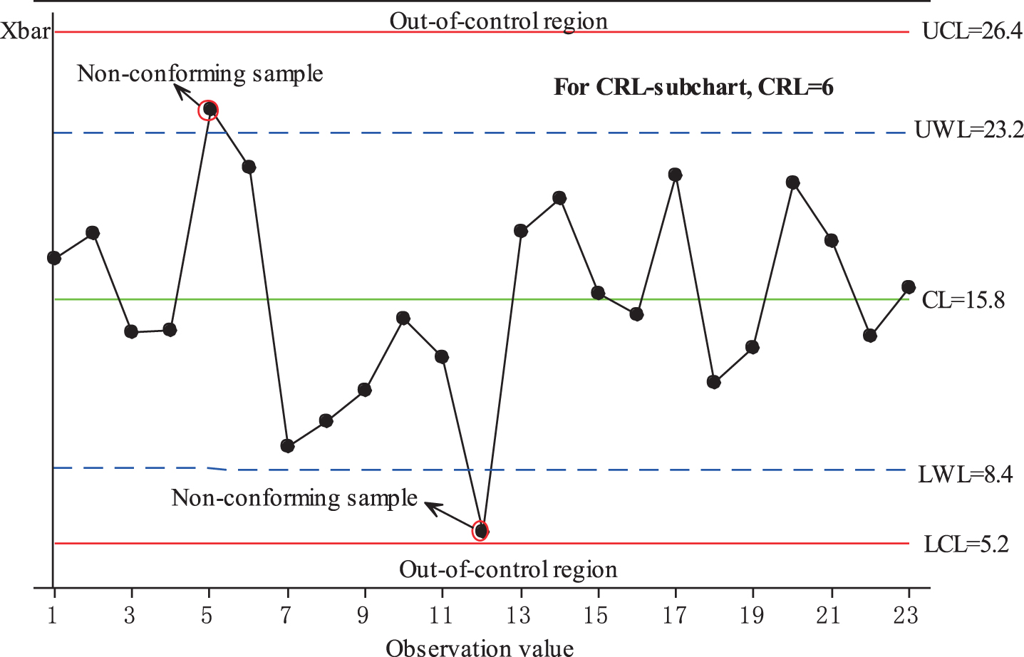
A graphical illustration of the FSI synthetic $\bar{X}$ chart.

3.1 Performance indices

Besides ARL, another two statistical indices, namely average time to signal (ATS) and adjusted average time to signal (AATS), are also widely used to evaluate the statistical performance of the considered control chart.

Average Time to Signal (ATS), which refers to the average time from the start of the process to the time when an out-of-control signal is generated by the control chart. The in-control ATS, denoted as ATS₀, is designed by quality assurance (QA) engineers to satisfy the requirement on false alarm rate. The out-of-control ATS, denoted as ATS₁, is the expected value of the time to signal that the process is out of control when a process shift has occurred.

Adjusted Average Time to Signal (AATS), which is defined as the expected time from the process mean shift to the time when the shift is truly signaled.

In this section, the Markov chain approach proposed by Davis and Woodall [9] is employed to compute the ARL, ATS and AATS of the VSI synthetic chart.

Let p₁ denote the probability that a non-conforming $\bar{X}$ sample occurs, that is, the probability that a sample falls in the out-of-control region of the $\bar{X}$ sub-chart. p₁ can be computed as $p_{1} = 1 - Φ (k_{1} - δ \sqrt{n}) + Φ (- k_{1} - δ \sqrt{n})$ (8) where Φ (·) is the cumulative distribution function of a standard normal random variable.

Let p₂ and p₃ denote the probability that a sample falls in the warning region and the central region of the $\bar{X}$ sub-chart, i.e. (UWL, UCL) ∪ (LCL, LWL) and (LWL, UWL), respectively. Then they can be respectively computed as $\begin{matrix} p_{2} & = Φ (k_{1} - δ \sqrt{n}) - Φ (k_{2} - δ \sqrt{n}) + \\ Φ (- k_{2} - δ \sqrt{n}) - Φ (- k_{1} - δ \sqrt{n}) \end{matrix}$ (9) $p_{3} = Φ (k_{2} - δ \sqrt{n}) - Φ (- k_{2} - δ \sqrt{n})$ (10)

Then a Markov chain {N (i) , i ≥ 1} can be constructed to describe the VSI synthetic $\bar{X}$ control chart scheme, where N (i) represents the number of samples which fall within the central control limits between the ith and the (i - 1)th sample which falls within the warning control limits of the $\bar{X}$ sub-chart. According to the analysis above, the state space of the Markov chain is {0, 1, 2, . . . , L - 1, L, S}, where state S implies that the chart triggers an out-of-control signal. In detail, a {L + 2, L + 2} transition probability matrix P can be constructed to model the VSI synthetic $\bar{X}$ control chart, which has the following structure: $P = (\begin{matrix} 0 & p_{3} & 0 & \dots & \dots & 0 & 0 & p_{2} + p_{1} \\ 0 & 0 & p_{3} & ⋱ & 0 & 0 & p_{2} + p_{1} \\ ⋮ & ⋮ & ⋱ & ⋱ & ⋱ & ⋮ & ⋮ & ⋮ \\ ⋮ & ⋮ & ⋱ & p_{3} & 0 & 0 & p_{2} + p_{1} \\ 0 & 0 & \dots & \dots & 0 & p_{3} & 0 & p_{2} + p_{1} \\ p_{3} & 0 & \dots & \dots & 0 & 0 & 0 & p_{2} + p_{1} \\ 0 & 0 & \dots & \dots & 0 & 0 & 0 & 1 \end{matrix}) = (\begin{matrix} Q & r \\ 0^{T} & 1 \end{matrix})$ (11) where Q is the (L + 1, L + 1) matrix of transient probabilities and 0 = (0, 0, …, 0) ^T. The (L + 1, 1) vector r = 1 - Q · 1 with 1 = (1, 1, …, 1) ^T. Then the expect value of ARL can be given by $ARL = q^{T} (I - Q)^{- 1} 1$ (12) where I is a (L + 1, L + 1) identity matrix, and q is a (L + 1, 1) vector of initial probabilities related to the transient states, with 1 for the initial state and 0 elsewhere. In this paper, we assume q = (0, 1, 0, …, 0) ^T. Then ARL₁ can be worked out by substituting the value of δ > 0 into equations (8-10), while ARL₀ can be worked out by substituting δ = 0 into equations (8-10).

For calculating the ATS and AATS of the chart, the steady-state probability of the process is required due to the uncertainty of the instantaneous probability of the process in each state.

Let π = {π₀, π₁, . . . , π_L} be the homologous steady-state probability of the state space. Based on Markov theory, the following results can be obtained: ${\begin{matrix} π_{0} = 1 - p_{3}, \\ π_{i} = p_{3}^{i} (1 - p_{3}), & i = 1, 2, . . ., L - 1, \\ π_{L} = p_{3}^{L} \end{matrix}$

Then when the size of the mean shift is δ (≥0), the expected value of the average sampling interval Eh (δ) can be given by $Eh (δ) = π_{0} h_{0} + (π_{1} + π_{2} + . . . + π_{L}) h_{1}$ (13)

The ATS of VSI synthetic $\bar{X}$ chart then can be given by $ATS = ARL \times Eh (δ) .$ (14) Similarly, the in-control ATS, denoted byATS₁, can be calculated by substituting δ ≠ 0, while the out-of-control ATS, denoted by ATS₀, can be computed by substituting δ = 0.

Carot et al. [4] assumed that the sojourn interval of the in-control state of process follows a uniform distribution for the calculation of AATS. The same assumption is adopted here. Then the AATS of VSI synthetic $\bar{X}$ control chart for a specific shift size δ (>0) can be given by $AATS = ({ARL}_{1} - 0.5) \times Eh (δ)$ (15)

4 The VSI synthetic

\bar{X}

control chart with estimated parameters

Most of control charts are designed under the assumption that the process parameters are known. However, these parameters are almost impossible to be known and they have to be estimated from an in-control reference sample. In this section, we reconstruct the VSI synthetic $\bar{X}$ control chart under the assumption that process parameters are estimated. In this case, the operation of the proposed chart is unchanged but the calculation of control limits of the $\bar{X}$ sub-chart is changed. Undoubtedly, the performance of the VSI synthetic $\bar{X}$ control chart will be affected.

When the values of μ₀ and σ₀ are unknown, their estimators ${\hat{μ}}_{0}$ and ${\hat{σ}}_{0}$ should be adopted to design the control chart. In such condition, the control limits of $\bar{X}$ sub-chart become $UCL = {\hat{μ}}_{0} + k_{1} {\hat{σ}}_{\bar{X}}, UWL = {\hat{μ}}_{0} + k_{2} {\hat{σ}}_{\bar{X}}$ (16) $LWL = {\hat{μ}}_{0} - k_{2} {\hat{σ}}_{\bar{X}}, LCL = {\hat{μ}}_{0} - k_{1} {\hat{σ}}_{\bar{X}}$ (17) where ${\hat{σ}}_{\bar{X}} = \frac{{\hat{σ}}_{0}}{\sqrt{n}}$ .

These two estimators ${\hat{μ}}_{0}$ and ${\hat{σ}}_{0}$ are calculated based on an in-control reference sample of m subgroups of size n. Assuming that the observations sampled from the process are independent and identically distributed normal random variables. The estimator ${\hat{μ}}_{0}$ for μ₀ and the estimator ${\hat{σ}}_{0}$ for σ₀ then can be respectively calculated as

${\hat{μ}}_{0} = \frac{1}{mn} \sum_{i = 1}^{m} \sum_{j = 1}^{n} X_{ij}$ (18) ${\hat{σ}}_{0} = \sqrt{\frac{\sum_{i = 1}^{m} \sum_{j = 1}^{n} (X_{ij} - \bar{X_{i}})^{2}}{m (n - 1)}}$ (19) where X_ij is the jth unit from subgroup i, and $\bar{X_{i}}$ is the sample mean associated with the ith sample, that is $\bar{X_{i}} = \frac{1}{n} \sum_{j = 1}^{n} X_{ij}$ (20)

When process parameters are known, the control limits of VSI synthetic $\bar{X}$ chart are regard as constants. However, they will be regard as random variables in the case where estimated process parameters are used. Therefore, the calculation of ARL, ATS and AATS in the estimated-parameter case will be different with the known-parameter case.

4.1 Performance indices in the estimated parameters case

In the case where process parameters are estimated, the approach proposed by Zhang et al. [31] is adopted to compute the ARL of VSI synthetic $\bar{X}$ control chart.

The estimators ${\hat{μ}}_{0}$ and ${\hat{σ}}_{0}$ for μ₀ and σ₀ can be achieved by the method introduced above. When ${\hat{μ}}_{0}$ and ${\hat{σ}}_{0}$ are given, the conditional probability ${\hat{p}}_{1}$ , ${\hat{p}}_{2}$ and ${\hat{p}}_{3}$ (corresponding to p₁, p₂ and p₃ in the known-parameter case) for $\bar{X}$ sub-chart can be respectively calculated as ${\hat{p}}_{1} = Φ (- U - k_{1} V + δ \sqrt{n}) + Φ (U - k_{1} V - δ \sqrt{n})$ (21) $\begin{matrix} {\hat{p}}_{2} & = Φ (U + k_{1} V - δ \sqrt{n}) - Φ (U + k_{2} V - δ \sqrt{n}) \\ + Φ (U - k_{2} V - δ \sqrt{n}) - Φ (U - k_{1} V - δ \sqrt{n}) \end{matrix}$ (22) ${\hat{p}}_{3} = Φ (U + k_{2} V - δ \sqrt{n}) - Φ (U - k_{2} V - δ \sqrt{n})$ (23) where $U = ({\hat{μ}}_{0} - μ_{0}) \frac{\sqrt{n}}{σ_{0}}$ (24) $V = \frac{{\hat{σ}}_{0}}{σ_{0}}$ (25)

Because ${\hat{μ}}_{0}$ follows a normal distribution with mean μ₀ and variance $\frac{σ_{0}^{2}}{mn}$ , i.e. ${\hat{μ}}_{0} \sim N (μ_{0}, \frac{σ_{0}^{2}}{mn})$ , then we have $U \sim N (0, \frac{1}{m})$ . The probability density function of U then can be deduced as $f_{U} (u | m) = f_{N} (u | 0, \frac{1}{m})$ (26) where $f_{N} (\cdot | 0, \frac{1}{m})$ is the probability density function of the normal distribution with mean 0 and variance $\frac{1}{m}$ .

Because $\frac{{\hat{σ}}_{0}^{2}}{σ_{0}^{2}}$ follows a gamma distribution with shape parameter $\frac{m (n - 1)}{2}$ and rate parameter $\frac{2}{m (n - 1)}$ , i.e. $\frac{{\hat{σ}}_{0}^{2}}{σ_{0}^{2}} \sim γ (\frac{m (n - 1)}{2}, \frac{2}{m (n - 1)})$ , then it can be concluded that $V^{2} \sim γ (\frac{m (n - 1)}{2}, \frac{2}{m (n - 1)})$ (27) Consequently, the probability density function of V can be deduced as $f_{V} (v) = 2 {vf}_{γ} (v^{2} | \frac{m (n - 1)}{2}, \frac{2}{m (n - 1)})$ (28) where f_γ (·) is the probability density function of the gamma distribution with parameters $\frac{m (n - 1)}{2}$ and $\frac{2}{m (n - 1)}$ .

The unconditional ARL and ATS under the case of process parameters estimation then can be calculated as $\begin{matrix} ARL & = \int_{- \infty}^{\infty} \int_{0}^{\infty} q^{T} (I - Q)^{- 1} 1 \\ \times f_{U} (u | m) f_{V} (u | m) dvdu \end{matrix}$ (29) $\begin{matrix} ATS & = \int_{- \infty}^{\infty} \int_{0}^{\infty} Eh (δ) q^{T} (I - Q)^{- 1} 1 \\ \times f_{U} (u | m) f_{V} (u | m) dvdu \end{matrix}$ (30) $AATS = ({ARL}_{1} - 0.5) \times Eh (δ > 0)$ (31) where the notations Q and Eh (δ) are the same as defined in Subsection 3.1 but by adopting the conditional probability. Similarly, the ARL₁ and ATS₁ are calculated by substituting the desired δ ≠ 0, while the ARL₀ and ATS₀ are computed by substituting δ = 0.

5 Design model

In order to obtain the optimal design parameters of VSI synthetic $\bar{X}$ control chart, the statistical design of VSI synthetic $\bar{X}$ control chart is conducted, which uses the following optimization model: $\begin{matrix} Objective function : & Min AATS \\ Constraints : & ATS0 =τ \\ h_{max} > h_{0} \geq h_{1} > 0 \\ k_{1} \geq k_{2} > 0 \\ n, L \in Integer value \\ Design variable : & k_{1}, k_{2}, h_{0}, h_{1}, L, n . \end{matrix}$ (32) where τ and h_max are, respectively, the allowed minimum in-control average run length to signal and the maximum sample size. The value of τ is usually decided by the QA engineer in regard to the false alarm rate.

5.1 Design procedure

As we can see, it is computationally complex to optimize the proposed statistical design model because the model is a non-linear model with mixed continuous-discrete decision variables. Genetic Algorithm (GA) is widely used in solving such optimization problems. Recently, successful applications of GA in the optimal design of control charts can be found in Bezerra et al. [2], Kosztyán and Katona [15], Wan et al. [25, 26], and so on. In this paper, a GA is constructed to solve the proposed model.

In the processing of using a GA, crossover operator and mutation operation are two crucial parameters that need to be set up. The values of these two parameters were determined by trial and error in our GA. Specifically, the population number, crossover rate, and mutation rate are set up to 700, 0.7 and 0.3, respectively. For our experiment, the solution process using the developed GA by MATLAB 8.3.0(R2014a) is concisely described as follows:

Initialization: At the start of the GA procedure, 700 candidate solutions which meet the constraint condition of the parameter of individual test are randomly generated. Specifically, the constraint condition stand for individual test parameter is given below: $1 \leq n \leq 10, 0 < h_{1} < h_{0} \leq 2,$ $0 < k_{2} < k_{1} \leq 3, 1 \leq L \leq 20$

Evaluation: In this step, the fitness of individual solution is defined by computing the value of fitness function. For this study, the fitness function is shown in Eq.(32).

Selection: Based on the fitness expression obtained in Step 2, 100 solutions that are probably going to be better fitness of solutions. Then these solutions are selected to breed the next generation. (In the selection, the chromosome with the lower AATS value is used to replace the higher AATS chromosome.)

Crossover: During this phase, a pairs of parent solutions which come from the 100 solutions are chose randomly and employed for crossover operations to produce the new chromosomes of the next generation. In our experiment, the arithmetical crossover method with crossover probability 0.7 is adopted, which has the following form: $Θ_{1} = 0.7 F + 0.3 M, Θ_{2} = 0.3 F + 0.7 M$ where Θ₁ represents the first new chromosome, Θ₂ represents the second new chromosome, and F and M are defined as the parents chromosomes. Thus, 200 children are produced when 100 randomly selected parents are used. Then, for next generation, the population size of 300 solutions are obtained.

Mutation: The mutation rate used in this research is 0.3. The non-uniform method is employed to carry out the mutation operation. As mentioned above, there are 300 candidate solutions. Then, ninety chromosomes (i.e., 300 × 0.3 = 90) can be randomly chose to mutate some genes.

Repeat the procedure from Step 2 to Step 5 until a stopping criterion is satisfied.

6 Performance comparisons

To investigate the performance of the VSI synthetic $\bar{X}$ chart for detecting the range process mean shifts in both the known and estimated process parameters cases, some comparisons are carried out in this section.

6.1 The comparisons between VSI and FSI synthetic $\bar{X}$ charts in the known-parameter case

As a general rule, if a control chart has smaller AATS value when a specific process mean shift δ is given, the control chart is considered better than its competitors, under the assumption that the same ATS₀ value is assigned to all considered charts. In this paper, for a fair comparison between the VSI and FSI synthetic $\bar{X}$ control chart schemes, both two control charts are designed to maintain the equation ARL₀=ATS₀=370.4 (that is Eh (δ = 0) =1). The values of input parameter δ ∈ {0.2, 0.4, 0.8, 1.5, 2.0} are used in the following numerical analysis. Then the comparison of AATS for the VSI and FSI synthetic $\bar{X}$ control charts in the known process parameters case are conducted and the numerical results are summarized in Table 2. Define that $χ % = \frac{{AATS}_{F} - {AATS}_{V}}{{AATS}_{F}} \times 100 % .$ (33)

Table 2

A comparison between the VSI and FSI synthetic $\bar{X}$ charts in accordance with AATS performance for δ ∈ {0.2, 0.4, 0.8, 1.5, 2.0}.

Shift size (δ)	VSI synthetic $\bar{X}$ chart							FSI synthetic $\bar{X}$ chart					χ%
	n	h ₀	h ₁	k ₁	k ₂	L	AATS _V	n	h	k	L	AATS _F
0.2	10	1.27	0.24	1.98	1.46	8	214.2	7	1	1.49	7	253.8	15.6%
0.4	7	1.65	0.54	1.84	1.12	13	73.2	7	1	1.24	8	84.8	13.7%
0.8	8	1.15	0.87	2.24	1.08	8	17.4	9	1	1.89	10	19.4	10.3%
1.5	8	1.42	0.72	2.10	1.48	10	1.3	8	1	1.58	14	1.4	7.1%
2.0	6	1.54	0.67	1.97	1.55	7	0.6	8	1	1.48	11	0.64	6.3%

From Table 2, from the aspect of time up to signal, it is obvious to see that the VSI synthetic $\bar{X}$ control chart substantially improves the detection efficiency of FSI synthetic $\bar{X}$ control chart. Especially, it greatly improves the detection ability for small and moderate process shifts. For example, when the true magnitude of the process mean shift δ is 0.2 (small mean shift), the FSI synthetic $\bar{X}$ chart takes 253.8 to give a signal. However, the VSI synthetic $\bar{X}$ chart only takes 214.2, which is 15.6% faster than the FSI synthetic $\bar{X}$ chart, showing that the VSI strategy is helpful in reducing the time to signal a process shift. Taken as a whole, the numerical results show that the capability of the VSI synthetic chart in yielding average performance boost of 16.4%, in the AATS of VSI synthetic $\bar{X}$ chart compared to the situation in which FSI synthetic $\bar{X}$ chart is used.

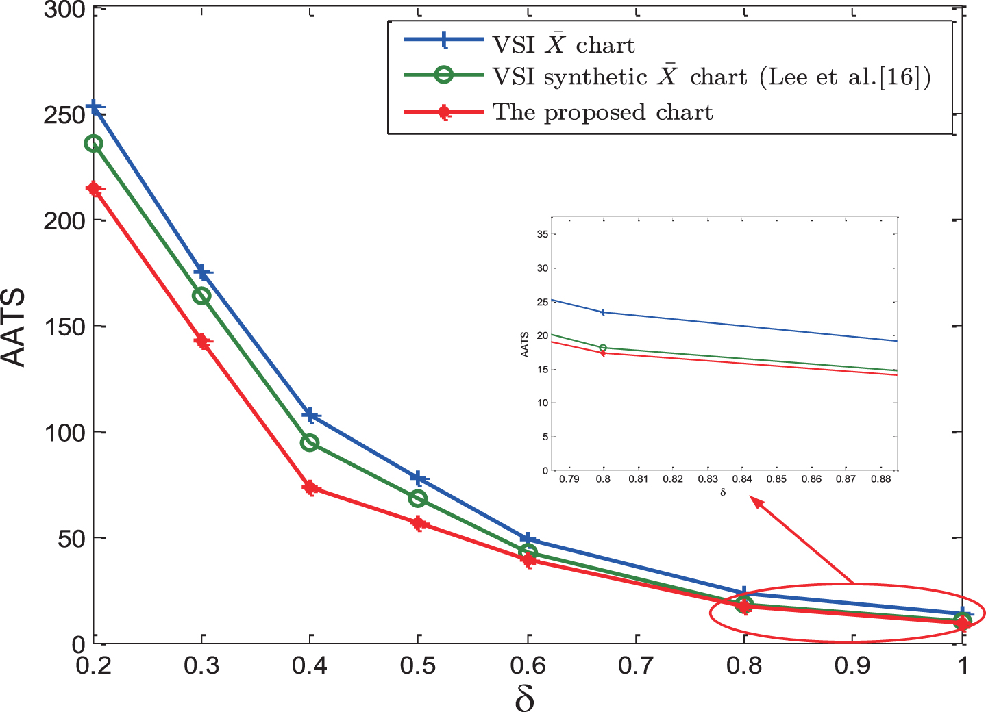
The comparisons between other VSI $\bar{X}$ type control charts (including the VSI $\bar{X}$ chart and Lee et al. [16]’s VSI synthetic $\bar{X}$ chart) and our proposed chart are also carried out. The results (in terms of AATS) are depicted in Figure 6. Without loss of generality, all of these charts are set to maintain the equation ATS₀ = 370.4 so that a fair comparison can be made.

Fig. 6

AATS for the VSI $\bar{X}$ , VSI synthetic chart proposed by Lee et al. [16] and our proposed chart when ATS₀ = 370.4.

From Figure 6, it is clear that the proposed synthetic $\bar{X}$ chart is superior to the VSI synthetic chart proposed by Lee et al. [16] and the VSI $\bar{X}$ chart for all considered process mean shifts. It is noteworthy that the proposed chart obtains a more superior performance compared to the other two charts in detecting small-to-moderate process shifts. But when the mean shifts are large enough, the performance of all these control chart is very similar, especially for Lee et al. [16]’s VSI synthetic chart and our proposed chart. Based on the above discussion, it can be demonstrated that the proposed control-chart scheme has the advantage of being sensitive to small changes in the mean.

6.2 The performance of the VSI synthetic

\bar{X}

chart in the estimated-parameter case

In this subsection, the effects towards AATS when the optimal parameters of VSI synthetic $\bar{X}$ chart with known process parameters are adopted in the AATS computation corresponding to the estimated process parameters case are studied. The values of input parameter δ ∈ {0.2, 0.4, 0.8, 1.5, 2.0} are used here. To this end, the AATS values are first calculated by adopting the control chart parameters optimised in the known-parameter case. However, in this situation, the in-control variance and mean are estimated from the number of subgroups m =10, 20, 40, and 80. The extreme case of m =+ ∞ is also considered and it corresponds to the known-parameter case.

Table 3 lists the AATS values and the increase in AATS values for the different number of subgroups. The increase in AATS is an increase from the optimal AATS obtained from the known-parameter case.

Table 3
AATS values and increase in AATS by using the optimal parameters corresponding to the known-parameter case when process parameters are estimated

δ m=10 m=20 m=40 m=80 m=+∞

AATS Increase AATS Increase AATS Increase AATS Increase AATS Increase

0.2 1032.5 114.6 714.5 46.7 413.4 35.1 275.9 20.7 214.2 0

0.4 547.3 77.3 215.4 22.3 125.3 19.7 89.4 13.2 73.2 0

0.8 93.2 48.2 56.8 18.9 44.4 10.5 23.1 8.6 17.4 0

1.5 17.6 23.1 10.4 10.2 8.5 7.4 2.6 5.4 1.3 0

2.0 2.6 8.7 1.9 4.6 1.4 2.7 1.2 1.3 0.6 0

δ	m=10	m=20	m=40	m=80	m=+∞
0.2	1032.5	114.6	714.5	46.7	413.4	35.1	275.9	20.7	214.2
0.4	547.3	77.3	215.4	22.3	125.3	19.7	89.4	13.2	73.2
0.8	93.2	48.2	56.8	18.9	44.4	10.5	23.1	8.6	17.4
1.5	17.6	23.1	10.4	10.2	8.5	7.4	2.6	5.4	1.3
2.0	2.6	8.7	1.9	4.6	1.4	2.7	1.2	1.3	0.6

From Table 3, it is found that when the values of mean shift sizes δ are small, the increase in AATS becomes quit large. When the number of subgroups is small, the result will be more obvious. The reason may be that small process mean shift sizes leads to a poorer run length performance when estimated process parameters are adopted, consequently increasing the value of AATS. It is also found that the increase in AATS is not large when a moderately large number of subgroups is employed (m ≥ 20), except for small process shift. That is to say, in this condition, the optimal control chart parameters obtained from the known-parameter case can still be applied to estimate the AATS when estimated process parameters are used, with only a minute increase in AATS. Whereas the optimal control chart parameters obtained from known process parameters case can not be applied to safely estimate the AATS when estimated process parameters are used, since the time to signal a process shift will be increased. Meanwhile, it is worthy of note that when a large m is used, the increase in AATS becomes smaller for all cases. This indicates that as m increases, the AATS corresponding to the estimated-parameter case comes to that of known process parameters.

As mentioned above, when the parameters obtained from the known-parameters case are applied in the AATS computation when estimated process parameters are used, an increase in AATS will occur. Then the producer may want to know that how many the number of m of preliminary in-control subgroups for process parameter estimation should be used in order to have approximately the same AATS value for both the known-parameter and estimated-parameter cases. Define that $Δ = \frac{{AATS}^{estimated} - {AATS}^{known}}{{AATS}^{known}} .$ (34)

Table 4 lists the minimum value m^* of satisfying Δ < 0.01, namely, such that the relative difference between the AATS corresponding to the estimated process parameters case and the AATS corresponding to the known process parameters case is not larger than 1%.

Table 4

Minimum values m^* of satisfying Δ < 0.01

Cases (δ)	m ^*
0.2	196
0.4	65
0.8	32
1.5	14
2.0	10

From Table 4, we can found that for small values of δ, the value of m^* satisfying Δ < 0.01 is quite large. Therefore, under these cases, the AATS difference between the estimated parameters and known parameters cases is small only when a large numbers of preliminary in-control subgroups is available. Conversely, for large values of δ, only a moderately large m^* should be used so that the AATS difference can be less than 1%.

Table 5 lists the AATS values which are calculated by employing the optimal parameters corresponding to the case of estimated process parameters and savings (with regard to the AATS values in Table 3). From Table 5, we find that the smaller the shift size and the smaller the number of subgroups m, the larger will be the savings. When one of the two parameters (i.e. δ and m) is big enough, the savings are small. In short, it can be concluded that in the case of estimated process parameters, the AATS calculated by using the optimal parameters associated with the case of estimated process parameters is always smaller than that of using the optimal parameters associated with the known process parameters case. Therefore, in the estimated process parameters case, due to the fact that the AATS decreases along with the increase of the number of subgroups m, a large amount of preliminary subgroups should be employed whenever possible.

Table 5

AATS values and savings when chart’s optimal parameters corresponding to the estimated process parameters case are used

δ	m=10		m=20		m=40		m=80		m=+∞
	AATS	Savings	AATS	Savings	AATS	Savings	AATS	Savings	AATS	Savings
0.2	1013.6	18.9	702.0	12.5	410.0	3.4	275.1	0.8	214.2	0
0.4	533.7	13.6	205.2	10.2	117.9	7.4	84.7	4.7	73.2	0
0.8	90.1	3.1	55.1	1.7	43.6	0.8	22.7	0.4	17.4	0
1.5	14.3	3.3	8.9	1.5	7.9	0.6	2.4	0.2	1.3	0
2.0	1.9	0.7	1.4	0.5	1.1	0.3	1.1	0.1	0.6	0

7 Conclusion

The main purpose of this study is to propose an improved VSI synthetic $\bar{X}$ control chart, and to discuss the effects of process parameters estimation on the statistical performance of the proposed chart. A Markov chain approach is used to compute the adjusted average time to signal (AATS) of the proposed chart. Then the statistical design of the VSI chart is developed and solved by a genetic algorithm. According to the numerical analysis, the main conclusions are as follows: (1) The proposed VSI synthetic $\bar{X}$ chart is superior to the corresponding FSI synthetic chart with respect to AATS. (2) The statistical performance of the VSI synthetic $\bar{X}$ chart is seriously affected by the estimation of process mean and variance, in particular for small process mean shifts. (3) The difference in the statistical performance (in terms of AATS) between the estimated-parameter case and the known-parameter case can be neglected if the number of subgroups m from Phase I is large enough.

As an attempt of improving the FSI synthetic $\bar{X}$ control chart, there are still some limitations of the paper. As future research, the proposed model can be extended in the following two directions: first, simultaneous monitoring of the process mean and variance of characteristics of quality, and second, considering a production/service process with multiple assignable causes to the developed model more suitable for real production/service environments.

Footnotes

Acknowledgments

We sincerely thank the anonymous reviewers for their valuable suggestions and comments. We also wish to thank the editor for handling this paper. This research is supported by the Soft Science Research Plan Project of Henan Province (202400410105), the Key Scientific Research Project of Colleges and Universities in Henan Province (20A630030) and the Nanhu Scholars Program for Young Scholars of XYNU.

References

Aslam

and Khan

, A new variable control chart using neutrosophic interval method-an application to automobile industry, Journal of Intelligent & Fuzzy Systems 36(3) (2019), 2615–2623.

Bezerra

E.L.

, Ho

L.L.

and da Costa Quinino

, Gs2: An optimized attribute control chart to monitor process variability, International Journal of Production Economics 195 (2018), 287–295.

Calzada

M.E.

and Scariano

S.M.

, A synthetic control chart for the coefficient of variation, Journal of Statistical Computation and Simulation 83(5) (2013), 853–867.

Carot

, Jabaloyes

and Carot

, Combined double sampling and variable sampling interval x chart, International Journal of Production Research 40(9) (2002), 2175–2186.

Castagliola

, Celano

and Chen

, The exact run length distribution and design of the s2 chart when the in-control variance is estimated, International Journal of Reliability, Quality and Safety Engineering 16(01) (2009), 23–38.

Chen

, The run length distributions of the R, s and s2 control charts when is estimated, Canadian Journal of Statistics 26(2) (1998), 311–322.

Cheng

X.-B.

and Wang

F.-K.

, VSSI median control chart with estimated parameters and measurement errors, Quality and Reliability Engineering International 34(5) (2018), 867–881.

Dargopatil

and Ghute

, New sampling strategies to reduce the effect of autocorrelation on the synthetic t2 chart to monitor bivariate process, Quality and Reliability Engineering International 35(1) (2019), 30–46.

Davis

R.B.

and Woodall

W.H.

, Evaluating and improving the synthetic control chart, Journal of Quality Technology 34(2) (2002), 200–208.

10.

Han

, Shang

, Shu

and Khan

A.J.

, Time series data intelligent clustering algorithm for landslide displacement prediction, Journal of Intelligent & Fuzzy Systems 35(4) (2018), 4131–4140.

11.

Haq

, Weighted adaptive multivariate cusum charts with variable sampling intervals, Journal of Statistical Computation and Simulation 89(3) (2019), 478–491.

12.

, Jiang

and Deng

, A distance-based control chart for monitoring multivariate processes using support vector machines, Annals of Operations Research 263(1-2) (2018), 191–207.

13.

Jensen

W.A.

, Jones-Farmer

L.A.

, Champ

C.W.

, Woodall

W.H.

, et al., Effects of parameter estimation on control chart properties: a literature review, Journal of Quality Technology 38(4) (2006), 349–364.

14.

Khoo

M.B.

, Teoh

W.L.

, Castagliola

and Lee

M.H.

, Optimal designs of the double sampling

\bar{X}

chart with estimated parameters, International Journal of Production Economics 144(1) (2013), 345–357.

15.

Kosztyán

Z.T.

and Katona

A.I.

, Risk-based x-bar chart with variable sample size and sampling interval, Computers & Industrial Engineering 120 (2018), 308–319.

16.

Lee

L.Y.

, Khoo

M.B.C.

, Teh

S.Y.

and Lee

M.H.

, A variable sampling interval synthetic xbar chart for the process mean, PloS one 10(5) (2015), e0126331.

17.

Lee

M.H.

and Khoo

M.B.

, The economic and economic statistical designs of synthetic double sampling x-bar chart, Communications in Statistics-Simulation and Computation, 48(8) (2019), 2313–2332.

18.

Maravelakis

, Panaretos

and Psarakis

, Effect of estimation of the process parameters on the control limits of the univariate control charts for process dispersion, Communications in Statistics-Simulation and Computation 31(3) (2002), 443–461.

19.

Mehmood

, Qazi

M.S.

and Riaz

, On the performance of x control chart for known and unknown parameters supplemented with runs rules under different probability distributions, Journal of Statistical Computation and Simulation 88(4) (2018), 675–711.

20.

Nguyen

H.D.

, Tran

K.P.

and Heuchenne

, Monitoring the ratio of two normal variables using variable sampling interval exponentially weighted moving average control charts, Quality and Reliability Engineering International 35(1) (2019), 439–460.

21.

Runger

G.C.

and Pignatiello

, Adaptive sampling for process control, Journal of Quality Technology 23(2) (1991), 135–155.

22.

Safe

, Kazemzadeh

and Gholipour Kanani

, A markov chain approach for double-objective economic statistical design of the variable sampling interval control chart, Communications in Statistics-Theory and Methods 47(2) (2018), 277–288.

23.

Shirke

D.T.

and Barale

M.S.

, A variable sampling interval sign chart for variability based on deciles, Communications in Statistics-Simulation and Computation, (2019), (preprint): 1–12.

24.

Tran

P.H.

, Tran

K.P.

and Rakitzis

, A synthetic median control chart for monitoring the process mean with measurement errors, Quality and Reliability Engineering International 35(4) (2019), 1100–1116.

25.

Wan

, Wu

, Zhou

and Chen

, Economic design of an integrated adaptive synthetic chart and maintenance management system, Communications in Statistics-Theory and Methods 47(11) (2018), 2625–2642.

26.

Wan

and Zhu

, Detecting a shift in variance using economically designed VSI control chart with combined attribute-variable inspection, Communications in Statistics-Simulation and Computation, (2019), (preprint):1–15.

27.

and Spedding

T.A.

, A synthetic control chart for detecting small shifts in the process mean, Journal of Quality Technology 32(1) (2000), 32–38.

28.

Yen

F.Y.

, Chong

K.M.B.

and Ha

L.M.

, Synthetictype control charts for time-between-events monitoring,e, PloS one 8(6) (2013), 65440.

29.

Yen

J.-N.

, Hung

H.-C.

, Hsu

H.-C.

and Lee

Y.-C.

, Systematic design an intelligent simulation training system: from learn-memorize perspective, Microsystem Technologies 24(10) (2018), 4137–4147.

30.

Yeong

W.C.

, Khoo

M.B.

, Yanjing

and Castagliola

, Economic-statistical design of the synthetic

\bar{X}

chart with estimated process parameters, Quality and Reliability Engineering International 31(5) (2015), 863–876.

31.

Zhang

, Castagliola

, Wu

and Khoo

M.B.

, The synthetic

\bar{X}

chart with estimated parameters, IIE Transactions 43(9) (2011), 676–687.

32.

Zhang

, Castagliola

, Wu

and Khoo

M.B.

, The variable sampling interval

\bar{X}

chart with estimated parameters, Quality and Reliability Engineering International 28(1) (2012), 19–34.

33.

Zhou

, Wan

, Zheng

and Zhou

, A jointadaptive np control chart with multiple dependent state sampling scheme, Communications in Statistics-Theory and Methods 46(14) (2017), 6967–6979.

34.

Zhou

, Jiang

and Wang

, Recognition of control chart patterns using fuzzy svm with a hybrid kernel function, Journal of Intelligent Manufacturing 29(1) (2018), 51–67.

Papers	Type of control chart		Type of sampling interval		Design method of control chart		Type of process parameters
	Synthetic chart	Others	FSI	VSI	Statistical	Economic-statistical	Known	Estimated
Wu and Spedding (2009)	$\sqrt \| \bar{X} & CRL$		√	√		√
Calzada et al. (2013)	√\|CV & CRL		√		√		√
Dargopatil and Ghute (2019)	√\|T² & CRL		√		√		√
Lee and Khoo (2019)	$\sqrt \| DS \bar{X} & CRL$		√			√	√
Lee et al. (2015)	$\sqrt \| \bar{X} & CRL$			√	√		√
Tran et al. (2019)	√\|Median chart & CRL		√		√		√
Yen et al. (2013)	√\|TBE & CRL		√		√		√
Nguyen et al. (2019)		√		√	√		√
Safe et al. (2018)		√		√		√	√
Aslam and Khan (2019)		√		√	√		√
Haq (2019)		√		√	√		√
Shirke and Barale (2019)		√		√	√		√
Yeong et al. (2015)	$\sqrt \| \bar{X} & CRL$		√			√		√
Cheng and Wang (2018)		√		√	√			√
Khoo et al. (2013)		√	√		√			√
Mehmood et al. (2018)		√	√		√			√
Zhang et al. (2012)		√		√	√			√
Castagliola et al. (2009)		√	√		√			√
Chen (1998)		√	√		√			√
Maravelakis et al. (2002)		√	√		√			√
Zhang et al. (2011)	$\sqrt \| \bar{X} & CRL$		√		√			√
The proposed paper	$\sqrt \| \bar{X} & CRL$			√	√			√

Monitoring the process mean using a synthetic X ¯ control chart with two sampling intervals

Abstract

Keywords

1 Introduction

6 Performance comparisons

6.1 The comparisons between VSI and FSI synthetic X ¯ charts in the known-parameter case

Footnotes

Acknowledgments

References

6.1 The comparisons between VSI and FSI synthetic $\bar{X}$ charts in the known-parameter case