Customer’s class transformation for profit maximization in multi-class setting of Telecom industry using probability estimation decision trees

Abstract

Telecom sector is hugely losing profits in different degrees due to various undesired classes of its customers. Churners, a certain class of customers shifting to the competitors, are the most undesired class of customers who are the predominant reason for the losses. Still, there are other classes of customers in this business who stay with the enterprise, but they are inactive in using the services and leading to uncertainty and an insignificant amount of profits. When data mining techniques are applied to such applications they produce customer models in the form of decision trees, etc. and provide customer’s class label only such as churner/non-churner. Furthermore, they only focus on improving the technical interestingness measures of prediction models. Thus, very limited research has been carried out on turning the prediction results into useful decision making actions. Consequently, some manual work by domain expert has to be done to postprocess the model to obtain the actionable knowledge for changing the customer from undesired class to the desired one. However, some of the existing works are suggesting the actions to convert the class of the customer from one category to another, but they have limitations in that they do not generalize to more than two classes. In this paper, a novel algorithm, which aptly fits the multi-class setting of Telecom sector, is presented that suggest actions to change the customer from an undesired class to a desirable one with maximum net profit. We explain our proposed method with the help of a case study of the Telecom sector. Empirical tests are conducted on the case study problem and also on UCI benchmark data and shown that our method is effective and scalable. With the help of comparison with state-of-the-art methods and substantial experiments, we demonstrate the efficiency of the proposed method.

Keywords

Data mining probability estimation decision trees actionable knowledge discovery decision making profit maximization,Telecom sector

1 Introduction

Telecom service providing industry is facing more competition in recent years. With enormous industry deregulation, customers of this sector are more transient and have more options and they are easily shifting to other service providers [21]. The trend which denotes the loss of a customer to competitors is known as customer ‘churning’ or ‘attrition’ which is leading to a huge fall in the profits of the service providers. Telecom industry is highly affected due to this nature of the customers. Therefore, stopping attrition, and increasing profits by taking necessary actions receives huge attention in this industry. Low service levels provided to the customer, aggressive competitive strategies, new products, regulations, not up to date with the technology etc., could be other reasons for churning in this sector. Acquiring new customers is really a tough task in any business rather than retaining existing customer. Hence, now the Telecom sector is focussing more on retaining their existing customers. Therefore, it is necessary to take essential steps to retain the customers in the Telecom sector. In general, retaining the existing customers is cheaper than acquiring new customers [13]. To remain profitable in their business, Telecom industry is consistently putting efforts to hold its customers. In this direction, it organizes customer retention campaigns with the objective of detecting which existing customers are intending to shift to the competitor and provide suitable offers and benefits to them to avoid churning. Telecom service providers normally have a huge number of customers, and therefore, detecting probable churners with the help of customer retention campaigns can be really a tough task. Hence, service providers are depending on churn prediction models of machine learning to find potential churners. When existing customers’ data (personal, demographic, behavioral details, and services provided, etc.), is given as input to the churn prediction model, it specifies which customers will be the likely churners. By using the output produced by the churn prediction model, the service providers with the help of domain experts do some manual work and can determine some possible personalized actions to make the likely churners satisfied and stay with them. Due to this reason, churn prediction models are vastly researched. For churn prediction, enterprises use various machine learning techniques [8 , 43] to discover the hidden patterns and relationships between instances and their features in huge data.

Many researchers of the machine learning community have proposed different techniques in order to handle the problem of churn prediction in the Telecom and other enterprises. They tried to provide a solution using methods like decision trees, Naive Bayes, Artificial Neural Networks, Support Vector Machines, and Rough Set approach etc. Out of these methods, decision tree based algorithms have often performed the best along with other ensemble methods [22]. In the context of CRM, the present research is aimed at building only the efficient churn prediction models on customers’ profiles and accurately classifying a customer as a churner or non-churner which does not offer direct benefit to the enterprise. The constructed model does not suggest any actions for churn prevention and profit maximization which is the final objective of the enterprises. Hence, it is necessary for the enterprises especially like Telecom service providers to use the services of the domain experts for performing some extra manual work on the model to discover actions for churn prevention and profit maximization. So far, very limited research has been done on automatic extraction of actionable knowledge using machine learning models to achieve the final objective of the enterprises.

If the discovered knowledge can directly suggest the fruitful actions to achieve the objective function without any additional manual efforts, then it is referred to as actionable knowledge [6]. Simply, an ‘action’ is changing the present value of an attribute of a customer to another possible value. However, each action incurs some cost to the enterprise. Attributes can also be described as changeable attributes and unchangeable attributes. Values of changeable attributes are possible to change by applying actions. In the Telecom sector, data plan, roaming plan, calls tariff etc. can be the examples of changeable attributes since the values of these attributes can be changed by the operator. On the other hand, the values of unchangeable attribute (Eg. Gender, age, marital status, etc.) are not possible to change. Intuitively, actionable knowledge discovery entails determining a finite number of actions in order to make changes to the values of the attributes of the input instance, so that its class is changed from undesired to a desired with a maximum net profit. In the Telecommunication industry, by using the machine learning model an existing customer can be predicted that he/she is more likely to switch to another service provider. Then, the actionable knowledge can be the actions to retain that unwilling customer such as reducing the call and SMS charges, providing free roaming services, increasing service level, and offering suitable data plan, etc.

Though some researchers worked on mining actionable knowledge for customer retention in this sector, they have some limitations. All the past researchers had seen the problem as a 2-class problem only and there was no specific focus on dealing the multi-class problems. The existing methods treated the customers of CRM applications belong to two classes (Churner and Non-churner) only and designed solution which fits for 2-class applications and tried to change ‘Churner’ as a ‘Non-churner’ [27 , 49]. Generally, Telecom sector also classify its customers according to the degree of profitability. In the Telecom business, there can be customers with more than two classes in a certain order of priority based on the degree of profitability. Hence, it is not necessary to restrict to the applications or domains with two classes of customers only. In Customer Relationship Management, in one scenario, customers are classified as platinum tier, gold tier, iron tier, and lead tier in the decreasing order of profitability [48]. In one another case, customers are classified as High loyal, latent loyal, spurious loyal and low loyal [7] where the ‘High loyal customers’ are of most profitable class and ‘low loyal’ are least profitable. In these cases, a customer who has fallen in a less profitable class has to be changed to any one of the possible higher level profitable classes with a maximum net profit. In such a way, when customers are of multiple classes in a certain order of priority based on the degree of profitability, then for the enterprises it is required to convert them from a lesser profitable class to a higher profitable class to improve the profits. Thus, solutions for the problems with more than two classes of customers are required. To the best our knowledge, the present research has not adequately addressed the customer’s class transformation issue when the number of classes of customers is ‘n’ where n > 2. This paper addresses these limitations and challenges and the main aim is predicting the churning nature and less profit yielding features of the customers and suggesting required actions to avoid churning or to change the customer from a lesser profitable class to a higher profitable class in the multi-class environment of Telecom sector.

We introduce our technique ‘Dest_leaf_finder’ which extracts actionable knowledge by post processing the probability estimation decision tree (PET). With the help of PET if an existing customer is predicted to be as a Churner or a low profitable class customer, then this method tries to convert him/her as non-churner/higher profitable class customer by changing the values of changeable attributes and also taking the cost of actions into account. The proposed PET based method treats the problem as a multi-class problem where n≥2. It provides profit maximization solution when the customers are classified according to the amount of profit earned from them. Eventually, the main objective of this paper is developing a model which assists the Telecom sector to transform churners as non-churners and changes less profit yielding customers as more profit yielding ones. The proposed method is presented as a case study using the real data pertaining to one Telecom operator in India, on customer’s class transformation for profit maximization. Experiments on real-world data and UCI datasets demonstrate that our method achieves finer computational performance while achieving the objective and outperforms the ensemble tree based state-of-the-art methods [32, 49] and also single tree based methods [27 , 34].

The rest of the paper is organized as follows: In Section 2 we review the literature and discuss the related work. In Section 3, we present some preliminaries and also discuss extracting knowledge from PET using our algorithm Dest_leaf_finder for 2-class, 3-class scenarios of Telecom and finally, a mathematical model has been formulated to provide the required solution for n-class context. In Section 4, performance evaluation of Dest_leaf_finder and run time comparisons with the state-of-the-art methods has been presented. In Section 5, we have given the conclusions and discussed the possibilities for the future work.

2 Related work

Churning problem in Telecom industry has been studied and addressed by many researchers earlier [1 , 40]. Data mining and machine learning community have widely studied on providing a solution and a model for forecasting attrition nature of customers where most of the focus is on improving the technical interestingness measures of the models [16 , 42]. In the past, many researchers have shown their interest on CRM and direct marketing problem and handled the cost-sensitive customer retention problem as a classification problem [32, 34]. B. Zadrozny and C. Elkan [47] described a method for cost-sensitive learning with the assumption that costs vary based on the examples.

The framework presented by Cui et al. [49] post-processes the additive tree model (ATM) classifier like random forest. Their method employs integer linear programming to determine measures for changing the class membership of a sample. They focused on changing the values of attributes without taking profit maximization into consideration. Qiang LU et al. [32] extended the work of Zhicheng Cui et al. [49] and presented a method which post processes ensemble of trees and finds actions with maximum net profit for a given single input instance. They also showed that finding optimal actions to transform an undesired class instance to a desired class from the ensemble of trees is NP-hard. They transferred the problem of finding optimal actionable plans to a state space graph search problem and solved it. Furthermore, for achieving the balance between search time and quality of the solution, they also proposed their second method viz. state space search algorithm which gives a sub-optimal solution. They also proved that the computation time for extracting optimal actions with their framework is more efficient than the framework of Zhicheng Cui et al. [49]. However, computation time to achieve objective function using ensemble based classification models like random forest, etc. are high, especially when the dataset size is very large. Lv Q et al. presented a method [26] for transforming the prediction label of an input instance by considering action costs. They have formulated the suboptimal action plan problem using an ensemble method works in two phases which is also computationally expensive.

Yang et al. [34, 35] presented a decision tree based greedy approximate solution for mining the required actions to change a group of undesirable class input instances whom they call as ‘unloyal customers’ to a desirable class(loyal) with a maximum net profit. They have also considered changing the values of the attributes to obtain maximum net profit, but however as the method is generating a huge number of actions leading to more complications in the computation. Liu et al. [24] introduced a method which first prunes and summarizes the discovered set of rules and then finds a small number of direction setting rules from which actionable knowledge can be discovered with a little manual effort. By incorporating business needs with a fuzzy machine learning model, L. Cao et al. presented a method [5] for actionable knowledge discovery. They have adopted a method based on fuzzy aggregation which has balanced both business needs and technical measures by re-ranking the discovered outputs. Nasrin Kalanat et al. [28] presented another fuzzy based method for discovering cost-effective actions from data. Their method assumes that in all cases continuous-valued attributes in the data are discretized in advance that leads to the disadvantage that using this crisp behavior can result in missing the best actions. To overcome this problem, they presented a method based on fuzzy set theory as they took the output from fuzzy decision trees, and produced actionable knowledge through automatic fuzzy post-processing. Their algorithm takes into account the fuzzy cost of actions, and further, attempts to maximize the fuzzy net profit. Later, they extended their work by assuming only the selected attributes as the flexible attributes and provided the other form of solution [27]. Though research on actionableknowledge discovery from data mining models is limited, some researchers have even shown their interest in surveying the existing methods [25, 50]. Dong X et al. proposed a method for mining actionable knowledge [45] from sequential patterns instead of a classification model. In the course of actionable knowledge mining, Kalanat N et al. presented a method in the other dimension which is suitable for graph data pertaining to social networks where there will be relationships between the objects [20].

In order to describe performance metrics which are integrated with the main intentions of the end users, a cost-benefit analysis methodology has been presented by Verbraken et al. [41]. Ronan et al. proposed a classification rule based framework [38] which address the concept of actionability. Their approach suggests actions to reduce the degree of the unsatisfactory situation by considering the quality and feasibility of actions. Nonetheless, all the existing research has perceived the problem as a 2-class problem only.

3 Mining profitable knowledge from probability estimation decision trees (PET’s) for Telecom application

In this section, first, some preliminaries regarding decision tree and PET construction are discussed. Then, we present our method ‘Dest_leaf_finder’ as a case study on Telecom business for customer’s class transformation for profit maximization. We start with a 2-class problem and then discuss a 3-class problem and finally present the mathematical model for the multi-class setting.

3.1 Decision trees

In the perspective of machine learning, modeling for customer churn prediction can be formulated as a classification problem. Since the decision tree is a powerful, prevalently used and most popular tool for classification, we use it as our classification model. When compared to other classification techniques, decision trees are easy to interpret as they can generate understandable rules. Training and classification phases of decision tree are simple and fast. Normally, decision trees produce good accuracy [14] and effectively handle high dimensional data. In the Telecom sector, customers’ data includes various kinds of features of customers such as socio demographic attributes (e.g., age, income, gender, culture, zip_code, job_status, education and nationality), behavioural information (e.g., service usage time, revenue, customer interaction with company for service), etc. This information is used to predict the customer’s churning or profitability nature. To construct decision tree for customer’s profiles, we have used the C4.5 algorithm [39] and gain ratio as the splitting attribute selection measure. During decision tree construction, for selecting splitting attribute at a node, gain ratio is a better choice than Information gain which is biased towards the attribute with a large number of outcomes. Information gain describes that what amount of information an attribute gives us regarding the class. The calculation of information gain with respect to an attribute ‘A’ is given in Equation (1) where ‘D’ is the dataset, ‘n’ is the number of classes of customers, ‘P_i’ is the probability that a randomly selected instance has class-i, ‘v’ is number of outcomes of attribute A and D_j is the data partition matching the j^th value of attribute ‘A’. $Info Gain (A) = Entropy (D) - {Info}_{A} (D)$ (1) $where, Entropy (D) = - \sum_{i = 1}^{n} (P_{i} * {log}_{2} P_{i})$ (2) and ${Info}_{A} (D) = \sum_{j = 1}^{v} (\frac{| D_{j} |}{| D |} \times {Entropy (D}_{j}))$ (3)

Gain ratio measure performs a kind of normalization to information gain using split information as shown in Equation (4) to overcome the drawback with Information gain method. Gain ratio with respect to attribute A is: $Gain Ratio (A) = \frac{Information Gain (A)}{SplitInfo (A)}$ (4) where, ${SplitInfo}_{A} (D) = - \sum_{j = 1}^{v} (\frac{| D_{j} |}{| D |} \times {log}_{2} (\frac{| D_{j} |}{| D |}))$ (5)

The attribute with the maximum gain ratio will be selected as the splitting attribute at a node of the tree. C4.5 is a remarkable decision tree construction algorithm that is most likely the data mining trump card which is widely used till today. This algorithm has become very popular as it has been ranked as #1 in the top 10 Algorithms in Data Mining [46]. When the model has to be built on a very large dataset, other sophisticated decision tree techniques like Random forest [4] can be enormously huge and deep. They also increase the computation time of our objective function. When the other popular single decision tree construction method viz. Decision stump [44] is considered, though it produces a very short tree its technical evaluation measures are not up to the mark. Hence, our profit maximization approach cannot be applied on such models. Even when compared with one of the other prominent single decision tree construction methods i.e. Random Tree, C4.4 is better since it produces shallower trees with better technical evaluation measures than that of Random Tree. Though highly accurate decision trees are essential, the focus of this work is not finding the next best algorithm for Decision Tree or PET construction. Due to this reason, we used the standard algorithm for tree construction which is also perfectly suitable to explain our research and easy tounderstand.

For PET construction, the improved version of C4.5 algorithm viz. C4.4 is used. C4.4 employs maximum likelihood estimate, a completely frequency based method, and applies Laplace correction for smoothing the extreme probabilities [31]. The probability of belonging to class C_i for a customer’s instance X which has fallen into a leafnode is: $P (C_{i} / X) = \frac{\sum_{j = 1}^{| D |} \partial (C_{j}, C_{i}) + 1}{| D | + n}$ (6)

If j^th instance belongs to class-i, then ∂ (C_j, C_i)=1, otherwise 0 and n is the number of classes, |D| is the number of instances in the dataset. When customers’ profiles are given as input to C4.4 algorithm, a PET is obtained. For example, Fig. 2 and Fig. 3 represent a class labeled decision tree and a PET respectively for the dataset shown in Table 2. After PET is introduced, its performance is evaluated using necessary metrics [15, 19].

3.2 Dataset

To apply our proposed method, we have used a real dataset pertaining to a Telecom operator in India. The dataset contains 15000 instances of their subscribers described by 40 features. Out of these 15000, ‘Churn’ customers are 2500. Attributes are divided into four groups: Socio demographic, behavioral, charges, and customer service levels. The summary of the main features of the dataset is presented in Table 1. The output attribute is a class label which specifies whether the customer has churned or stayed within a period of 3 months. Before using the data for experiments, necessary preprocessing steps (eg. data cleaning, data transformation, etc.) are performed. During the experiments, 10-fold cross-validation is used to evaluate the constructedmodel.

Table 1
Description of various features of the Telecom dataset

Feature category Feature name Description

Socio Age Age group of the customer

Demographic Gender Customer’s gender (Male, Female)

Income Customer’s annual income

Culture Culture of the customer

Job_status Whether the customer is employee or not.

Education Customer’s educational qualification

zip_code Zip code of the area in which customer is living

Nationality Nationality that the customer belongs to

Behavioral Calling behaviour Total Calling time per month

Data usage Total amount of data used by the customer per month

SMS usage Total number of messages sent per month

Customer interaction with company for service Number of calls made to customer care service center

Revenue Amount of revenue generated by the customer by services usage per month

Charges Levied SMS Charges Amount charged per short message

Call Charges_National Amount charged per second on National Calls ($)

Call Charges_International Amount charged per second on International Calls ($)

Internet/Data Amount charged per MB ($)

Other Charges for other services like ring tones, apps. etc. ($)

Customer Services Level Customer Complaint Time taken to resolve the complaint given by the customer

Internet connectivity/speed Internet speed in Mbps

Signal strength Voice clarity level

Coverage Level Network coverage areas

Voice Call drop rate On average number of voice calls dropped per month

SMS drop rate On average number of SMS’s dropped per month

Feature category	Feature name	Description
Socio	Age	Age group of the customer
Demographic	Gender	Customer’s gender (Male, Female)
	Income	Customer’s annual income
	Culture	Culture of the customer
	Job_status	Whether the customer is employee or not.
	Education	Customer’s educational qualification
	zip_code	Zip code of the area in which customer is living
	Nationality	Nationality that the customer belongs to
Behavioral	Calling behaviour	Total Calling time per month
	Data usage	Total amount of data used by the customer per month
	SMS usage	Total number of messages sent per month
	Customer interaction with company for service	Number of calls made to customer care service center
	Revenue	Amount of revenue generated by the customer by services usage per month
Charges Levied	SMS Charges	Amount charged per short message
	Call Charges_National	Amount charged per second on National Calls ($)
	Call Charges_International	Amount charged per second on International Calls ($)
	Internet/Data	Amount charged per MB ($)
	Other	Charges for other services like ring tones, apps. etc. ($)
Customer Services Level	Customer Complaint	Time taken to resolve the complaint given by the customer
	Internet connectivity/speed	Internet speed in Mbps
	Signal strength	Voice clarity level
	Coverage Level	Network coverage areas
	Voice Call drop rate	On average number of voice calls dropped per month
	SMS drop rate	On average number of SMS’s dropped per month

3.3 Finding optimal destination leaf node for profit maximization

In this section, we introduce our technique ‘Dest_leaf_finder’ which tries to produce retention/profit increasing actions for each customer of Telecom sector who is predicted to be churner/less profitable. Due to the values of its attributes, an instance falls into a particular leaf L of the tree which represents a class. If we want to it to fall into another leaf node, we simply have to change the values of required attributes. If the instance has fallen into a leaf node(‘Source leaf’) which represents an undesired/lesser profitable class, then the task of ‘Dest_leaf_finder’ is finding the best leaf node (‘Destination leaf’) among the other leaf nodes with desired/higher profitability class for this instance. For this purpose, algorithm extensively searches and finds the right destination leaf node with maximum net profit for this customer to shift to. Therefore, to shift/transform a customer’s instance from a lesser profitability class to a higher profitability class, ‘Dest_leaf_finder’ changes the values of the necessary attributes of that instance. For example, ‘Customer Service level’ is one of the important features in the Telecom sector which is a changeable attribute. For instance, if the customer is provided with ‘low’ service level, then we need to change his/her service level to ‘high’ or ‘medium’ to make the customer satisfied and stay with the enterprise. For the enterprise to increase ‘service level’ it incurs some cost. A cost matrix is maintained for every attribute, where each entry in it is the cost that incurs to change the value of the attribute from one state to another. Values of the cost matrix are obtained from the domain expert. If the outcomes of an attribute are n, then the order of cost matrix will be n×n. Each element C(i, j) in the cost matrix represents the cost incurred to change an attribute value from i to j. As the unchangeable attributes’ values are impossible to change, for those attributes, elements in the cost matrix are filled with very huge and unbearable cost values to avoid considering that attribute’s value change. However, unchangeable attributes must be included during the decision tree induction process, as they are important and can influence the class of the customer to a greater degree and cannot be discarded. For example, some of the features described in Table 1 pertaining to Telecom data viz., customer gender, age, and job_status, etc. are required to be included while constructing the model to predict the nature of the customer. Research framework of our method is shown in Fig. 1. The constructed PET, input instance and the output given by the PET are inputs to our proposedalgorithm.

Fig.1

Research Framework of ‘Dest_leaf_finder’.

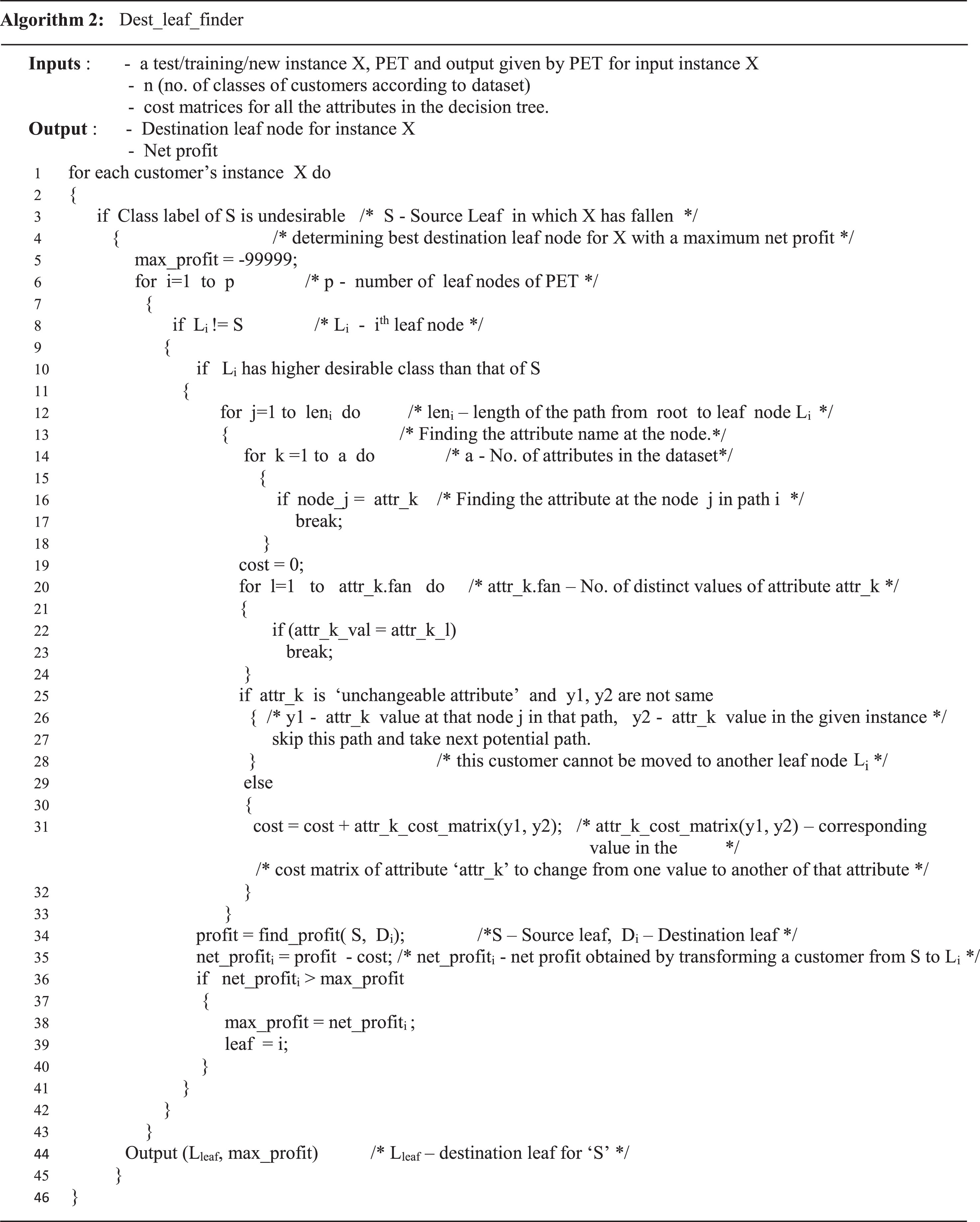
By using the PET, if a customer is predicted as belonging to a Churn/less profitable class, then while finding optimal destination leaf for him/her, Dest_leaf_finder algorithm considers each potential destination leaf node. At one time, from the PET, Dest_leaf_finder algorithm takes the path of one destination leaf node from root to leaf. Then it examines and finds the nodes’ (attributes’) values which do not match with the values of attributes’ of given input instance and thus identifies the actions. By considering the cost of actions, net profit will be computed for shifting the instance/customer from one leaf to another. This process is performed on all the potential destination leaf nodes and finally, the destination leaf and the corresponding actions which yield maximum net profit will be chosen. According to the procedure discussed above Dest_leaf_finder algorithm is designed and presented in Algorithm 2.

Source leaf for the input instance X is found using the algorithm find_leaf(). This algorithm takes one customer’s sample X i.e. test/training/new instance and according to its attributes’/features’ values, starting from the root the PET is traversed and an appropriate leaf node is reached.

Algorithm 1

find_leaf(X)
Input	: PET
Output	: Leaf node information of X
1	Traverse from root to leaf according to attribute values of instance X
2	return (Leaf node information of X)

Algorithm 2

Based on number of classes of the customers, the mathematical model for calculating the profit will be changed and the find_profit() method undergoes to slight changes.

Next, determining net profit in the three contexts of Telecom business is discussed. The first case discusses churn detection and prevention as a 2-class application, the second case discusses a 3-class application and finally finding profit for n-class (multi-class) scenarios is discussed and a mathematical model is formulated.

3.4 Case-1 : 2-class scenario of Telecom sector

Telecommunications industry broadly classifies its customers into two. One is ‘Non-churn’ customers who will stay with the same service provider. Another class of customers is ‘Churn’ customers who will cancel their account and shift to another service provider during a period of time. For easy illustration of proposed algorithm Dest_leaf_finder, we have used a small subset of the examples from the real Telecom dataset discussed in Section 3.2 to build the PET. Further, we have taken four significant input features i.e. service level, income of the customer, gender, and call charges belonging to different categories. Moreover, among these 4 attributes, 2 are changeable and 2 are unchangeable. Though call charges, service level have different sub categories we have generalized them for simplicity.

The description of the attributes of the subset of Telecom data is presented in Table 3. This dataset contains 14 instances composed of four significant categorical attributes of the customer and a class label viz., Churn, Non-churn. Among 14 instances of dataset, 9 are Non-churn (64.29%) and 6 are Churn (35.71%). Dataset in Table 2 is given as input to C4.4 algorithm and a class labeled decision tree (Fig. 2) and then a PET (Fig. 3) is obtained as output. The constructed tree describes customers with what kind of features will be of class ‘Churn’ and customers with what sort of features will be of class ‘Non-churn’. In the PET each leaf node also represents the class probabilities belonging to C₁ (Non-churn) and C₂ (Churn) if an instance has fallen in it. However, the leaf node is labeled with the majority class. Ultimately, for an instance which has fallen into a leaf node, the constructed PET can provide a class label and also the probability of belonging to each class. In our application, C₁ is the desirable class and C₂ is an undesirable class. In this case, we discuss changing the class of a customer from Churner (C₂) to Non-churner (C₁) i.e. C₂ → C₁ with a maximum netprofit.

Fig.2

Class labeled Decision Tree representing dataset inTable 2.

Fig.3

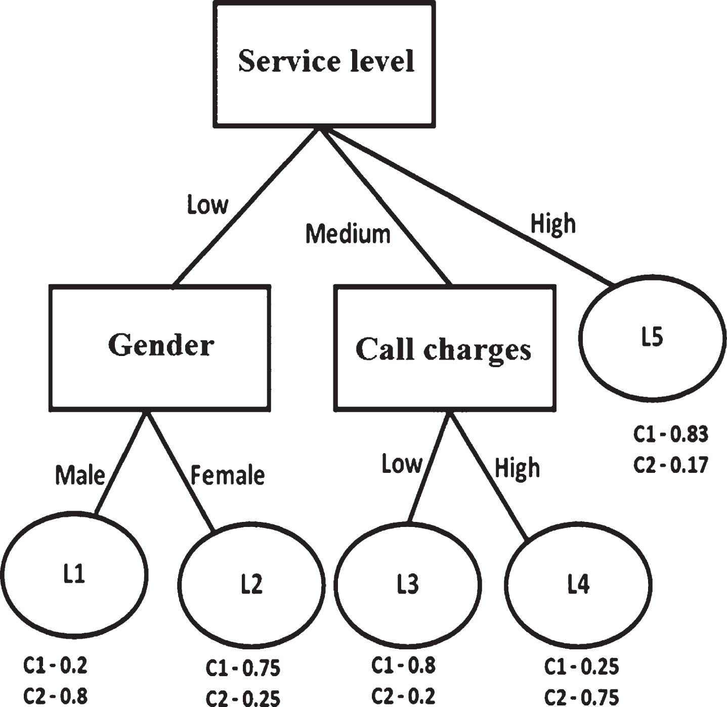
Probability Estimation Decision Tree (PET) representing dataset in Table 2.

Table 2

Sample 2-class dataset of Telecom

Service_level	Data usage	Gender	Call_charges	Class label
Low	High	Male	Low	Churn
Low	High	Male	High	Churn
High	High	Male	Low	Non-churn
Medium	Medium	Male	Low	Non-churn
Medium	Low	Female	Low	Non-churn
Medium	Low	Female	High	Churn
High	Low	Female	High	Non-churn
Low	Medium	Male	Low	Churn
Low	Low	Female	Low	Non-churn
Medium	Medium	Female	Low	Non-churn
Low	Medium	Female	High	Non-churn
High	Medium	Male	High	Non-churn
High	High	Female	Low	Non-churn
Medium	Medium	Male	High	Churn

Table 3

Description of Telecom data in Table 2

Feature	Description	Feature category	Changeable/unchangeable	Values
Gender	Gender of the customer	Demographic	Unchangeable	Male, Female
Data usage	Average amount of data used by the customer during a period of time	Behavioral	Unchangeable	Low, Medium, High
Service_level	Level of service provided to the customer	Customer Services Level	Changeable	Low, Medium, High
Call charges	Tariff on the calls made by the customer	Charges Levied	Changeable	Low, High
Class label	Whether customer churned or stayed	–	Changeable	Churn, Non-churn

In the case of 2-class problems of Telecom enterprise, if an instance/customer has fallen into a leaf node then profit obtained from him/her, if he/she remains in that leaf node, is computed with respect to the desirable class i.e Non-churn (C₁). If the probability of class C₁ is 1.0(if the customer is 100% Non-churn customer) for a leaf node, then enterprise makes a certain amount of profit ‘P_A’ from the customer who has fallen into this leaf. In our case study, we have considered a value $1000 for P_A which is obtained from a domain expert. As an example, if a customer falls into Leaf-1 (Fig. 4), then enterprise makes 0.8*1000 = $800.

Fig.4

A Leaf node representing probabilities w.r.t. 2-classes.

The method find_profit() called by Dest_leaf_finder algorithm computes the profit obtained by moving a customer from an undesired leaf node to a desired leaf node as shown in Equation (7). $P = P_{A} * (P_{C 1} (D) - P_{C_{1}} (S))$ (7)

In Equation (7), P is the profit obtained after shifting the customer from source leaf node S to destination leaf node D, and P_C₁(D) and P_C₁(S) are the probabilities of desirable class (Non-churn) if the customer is in destination leaf and source leaf respectively. P_C₁(D) and P_C₁(S) are obtained from i^th destination leaf D_i and source leaf S respectively. P_A is the amount of profit from a customer who is 100% in the desired class. However, by subtracting the total cost incurred for this transformation (since some actions have to be taken), the Dest_leaf_finder algorithm computes the net profit. For this case, find_profit() method is shown in Algorithm 3.

Algorithm 3

Finding profit for two class applications

find_profit(S, D_i) /* S-Source, D_i – Destination */

{

P = P_A * (P_C₁(D_i) – P_C₁(S))

return(P);

}

As an example, a customer’s instance X from our case study is considered, where the attribute values are Gender = Male, Data usage by the customer = High, Service_level = Low, Call charges = High. In the PET (Fig. 3), this instance falls into leaf node L1 which represents undesired class i.e. Churn. The possible destination leaf nodes for instance X can be L2, L3, and L5. We need to try out to which among them X can be moved to on changing its attribute’s values.

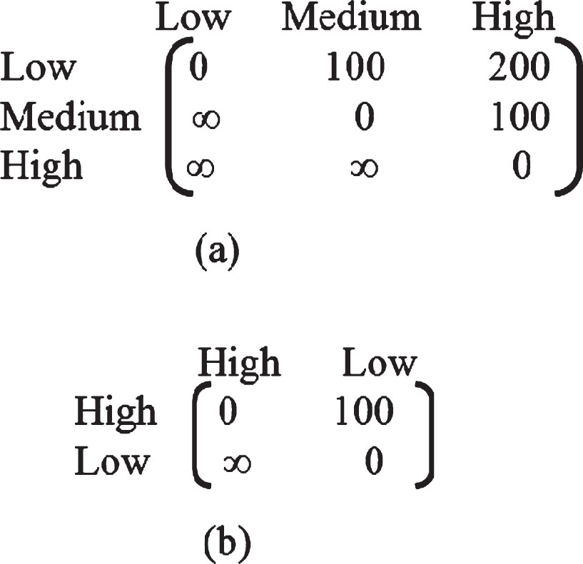
Cost matrices for the two changeable attributes in the PET (Fig. 3) i.e. Service_level and Call charges are given in Figs. 5(a) and 5(b) respectively. When we want to avoid changing the attribute’s value, a cost value ∞ has been taken. For example, changing ‘Service_level’ from ‘high’ to ‘low’ does not make any sense. Cost matrices of ‘Gender’ and ‘Data usage by customer’ are not given since they are not changeable attributes.

Fig.5

(a) Cost matrix of ‘Service_level’. (b) Cost matrix of ‘Call charges’.

X cannot be moved to L2 since the ‘gender’ (unchangeable attribute) has to be changed. X can be shifted to L3 by changing ‘Service_level’ from ‘Low’ to ‘Medium’ with the cost of $100 and ‘Call charges’ from ‘High’ to ‘Low’ with the cost of $100. Net profit in this case is (P_A * (P_C1(L3) - P_C1(L1))) – Total Cost=(1000 * (0.8-0.2)) – (100 + 100) = $400. Net profit obtained after transforming the customer X from L1 to L5 with one attribute’s value change i.e. ‘Service_level’ from ‘low’ to ‘high’ with the cost of $200 is (1000 * (0.83 – 0.20)) – 200 = $430. As the shift to L5 is yielding maximum net profit, L5 will be the destination leaf for X. Hence, for the customer X, source leaf node is L1, destination leaf is L5, action taken for transforming X from L1(undesired class) to L5 (desired class) is changing ‘Service_level’ from ‘low’ to ‘high’ and expected net profit after shifting is $430.

3.5 Case-2 : 3-class scenario of Telecom sector

Most often, Telecom sector finds a typical class of customers who do not cancel their account and continue with the same service provider but, they will be inactive in using the services. When a customer uses the enterprise services to a lesser degree and performs very less number of transactions every month, obviously profit obtained from him/her can be less. Due to various reasons like increased service charges, reduced coverage, the need for using data is finished, and unsatisfactory service levels, etc. can be reasons for this nature of the customer. However, these classes of customers cannot be ignored since they can be transformed as active customers by applying some cost-sensitive actions. Thus, in the real time scenario of Telecom sector, it is not necessary to restrict the customers to belong only to two classes like Non-churn or Churn.

Further, to study the additional behavior and profit-yielding nature of the customers, we have added a third class label viz., ‘Non-churn but less active’ and then 125 samples are collected from the customers of the same operator through structured questionnaires which are distributed online. This class of customers stays with the operator but inactive in using the services thereby lead to uncertainty and nominal profits. Each customer record is characterized by five decisive input attributes viz. SMS charges, call charges, internet connectivity/speed, service level, and signal strength. The details of the attributes of 3-class Telecom dataset are presented in Table 4. The class label of the customer can be one of the three labels viz. Non-churn and active customer (C₁), Non-churn but less active customer (C₂), Churn customer (C₃). Among 125 instances of dataset, 40 are C₁(32%), 42 are C₂(33.6%) and 43 are of class C₃(34.4%). After applying C4.4 algorithm on the dataset a PET which is shown in Fig. 8 is obtained. In this PET, each leaf node represents a class label (majority class) and also associated with each class probability of C₁, C₂, and C₃ respectively in the dottedbox.

Table 4
Description of attributes in the 3-class Telecom dataset

Feature/attribute Description Changeable/unchangeable Values

A1 SMS Charges Changeable A₁₁-High, A₁₂-Low

A2 Call Charges Changeable A₂₁-High, A₂₂- Low

A3 Internet connectivity/speed Changeable A₃₁-Good, A₃₂-Average, A₃₃ - Poor

A4 Service Level Changeable A₄₁-High, A₄₂ – Medium, A₄₃ – Low

A5 Signal strength/Voice clarity Changeable A₅₁-Low, A₅₂ – High

Class Class Label Changeable Non-churn and active customer(C₁), Non-churn but less active customer(C₂), Churn customer(C₃)

Feature/attribute	Description	Changeable/unchangeable	Values
A1	SMS Charges	Changeable	A₁₁-High, A₁₂-Low
A2	Call Charges	Changeable	A₂₁-High, A₂₂- Low
A3	Internet connectivity/speed	Changeable	A₃₁-Good, A₃₂-Average, A₃₃ - Poor
A4	Service Level	Changeable	A₄₁-High, A₄₂ – Medium, A₄₃ – Low
A5	Signal strength/Voice clarity	Changeable	A₅₁-Low, A₅₂ – High
Class	Class Label	Changeable	Non-churn and active customer(C₁), Non-churn but less active customer(C₂), Churn customer(C₃)

Here, class C₁(Non-churn and active customer) is the most preferred class. Class C₂(Non-churn but less active customer) is the next preferable class. Class C₃ represents churn customer i.e. Churner. Enterprise no longer can gain from the customer who belongs to class C₃. Obviously, there will be no profit for the enterprise if the C₃ probability is 1.0 because he/she leaves the enterprise. Accordingly, customers’ classes in the order of profitability in the descending are C₁, C₂, C₃. Our objectives are (1) to convert a customer who actually belongs to class C₂ to class C₁, and (2) converting a customer who belongs to class C₃ to either class C₁ or to class C₂ whichever is possible and more profitable to the enterprise. In 3-class problems, class transformations will be as shown below:

C₂→ C₁

C₃→ C₁/C₂

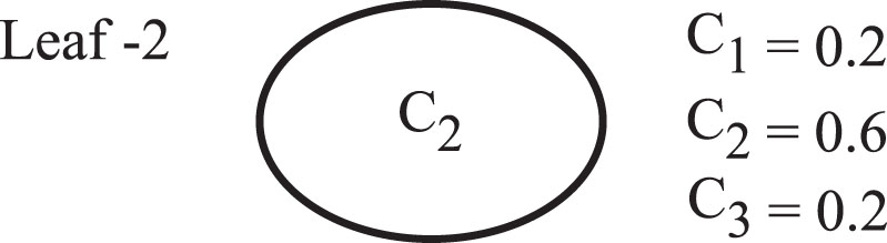
In a 3-class scenario of Telecom, when the customer has fallen into a leaf of the PET, the amount of profit obtained from him/her is computed in terms of probability of belonging to class C₁ and also class C₂. Though class C₁ is the most desired class, with respect to class C₂ also enterprise makes some amount of profit from the customer. Say, for instance, a leaf node Leaf-2 (Fig. 6) comprises the class probabilities C₁ = 0.2, C₂ = 0.6, C₃ = 0.2. This means, for a customer who has fallen into Leaf-2 contains the qualities of all the three classes in different degrees and also yields the profit with respect to each class except C₃. For instance, according to a domain expert, if C₁ probability is 1.0 then enterprise gains a profit of $1000 or if C₂ probability is 1.0 then the profit is $500. Hence, even if the customer purely belongs to class C₂, enterprise earns $500. However, a leaf can never have both C₁ probability 1.0 and also C₂ probability 1.0. In Fig. 6, the instance which has fallen into that leaf node will have ‘Non-churn and active’ class probability 0.2. Hence, with respect to class C₁, from him/her enterprise makes the profit of 1000*0.2 = $200. As the customer also has C₂ probability 0.6, with respect to this feature he/she yields a profit of 0.6*500 = $300. However, no profit can be gained with respect to class C₃ (Churner) probability which is 0.2, since this class represents that the customer will not stay with the enterprise. With respect to total staying probability, profit for the enterprise is 300 + 200 = $500. In this case, profit obtained from a customer by shifting him/her from an undesired leaf S to desired one D is, $\begin{matrix} P & = & (P_{A 1} * P_{C_{1}} (D) + P_{A 2} * P_{C_{2}} (D)) \\ - (P_{A 1} * P_{C_{1}} (S) + P_{A 2} * P_{C_{2}} (S)) \end{matrix}$ (8)

Fig.6

A Leaf node representing probabilities w.r.t. 3-classes.

In Equation (8), P_A1 is the profit if C₁ probability is 1.0 (100% class C₁ customer), P_A2 is profit if C₂ probability is 1.0 (100% class C₂ customer), P_C₁(D) and P_C₁(S) are class C₁ probability in destination leaf and source leaf respectively, P_C₂(D), P_C₂(S) are class C₂ probability in destination and source leaf nodes respectively. The procedure for calculating net profit for changing the customer’s instance from source leaf S to i^th destination leaf D_i in the case of 3-class problems is given in Algorithm 4.

Algorithm 4

Finding profit for three class applications
find_profit(S, D_i)
{
P=(P_A1P_C₁(D_i)+P_A2P_C₂(D_i)) - (P_A1P_C₁(S)+P_A2P_C₂(S))
return(P);
}

A customer’s instance Y is considered, which has fallen into the leaf L1 according to its attributes’ values, which represents the undesired class (Churner) as shown in Fig. 7. We can consider L2 as one of the potential destination leaf nodes for customer Y as its class label is C₁ which is most desirable. Here we proceed with the assumptions; if the customer’s C₁ class probability is 1.0 then profit is $1000, C₂ class probability is 1.0 then profit is $500. Based on the class probability values of the leaf node, profit, when Y has fallen into L1, is 1000*0.2 + 500*0.1 = $250. Profit if any instance falls into L2 is 0.8*1000 + 0.1*500 = $850. The difference in the profit if the instance is shifted from L1 to L2 is 850–250 = $600.If the cost incurred for the actions to shift from L1 to L2 is $200, then the net profit will be 600–200 = $400. In a similar fashion, we find the expected net profit after moving to other potential destination leaf nodes. Whichever the leaf yields maximum net profit; to that leaf customer Y is shifted.

Fig.7

3-class example.

For detailed illustration, an instance of customer Z belonging to our case study is considered, where attributes’ values are A1 = A₁₁, A2 = A₂₂, A3 = A₃₁, A4 = A₄₁, A5 = A₅₂. According to the suggestion of a domain expert in the Telecom business, profits of $1000 and $500 are considered if the customer’s C₁ class and C₂ class probabilities are 1.0 and 1.0 respectively. Action costs of the attributes are taken in the range of $[0–200].

In the PET shown in Fig. 8, Z falls into the leaf node L5 which is less profitable leaf with class C₂. Profit obtained from Z if he/she remains in L5 is (P_A1*P_C₁(S) + P_A2*P_C₂(S)) = 1000*0.28 + 500*0.57 = $565. An attempt is made to find the best destination node for customer Z with a maximum net profit. Z cannot be moved to L1 since its class label is also C₂. Moreover, L1’s C₁ and C₂ probabilities also lesser than that of L5’s. Instance cannot be moved to L2 or L3 or L4 since these leaf nodes’ class label is C₃ which is completely undesirable. Net profit, if Z is moved to L6 is [(1000 * 0.8 + 500 * 0.1) – 565] – 50 = $235. (Only attribute ‘A1’ value to be changed from A₁₁ to A₁₂. Cost for this change is $50 from the cost matrix of A1). Z cannot be moved to L7 which is undesirable leaf node (Class C₃). Net profit, if Z is moved to L8 is [(1000 * 0.7 + 500 * 0.1) – 565] – (100 + 50) = $35. Two attribute values are changed. Attribute A1 value is changed from A₁₁ to A₁₂ and attribute A3 value is changed from A₃₁ to A₃₂. Net profit, if this customer is moved to L9 will be [(1000 * 0.54 + 500 * 0.42) – 565] – 100 = $85. Only one action i.e. A3 value is changed from A₃₁ to A₃₃ is required. Further, no other leaf nodes among L10, L11, L12, L13, L14, L15, L16 or L17 yields a profit if Z is shifted to them. Z is moved to leaf L6 to obtain maximum net profit. Eventually, source leaf node for the instance Z is L5, destination leaf is L6 with Net Profit = $235 with one action on attribute A1 whose value is changed from A₁₁ to A₁₂. In this example, customer is transformed from class C₃ to C₁. It can be concluded that our proposed method works well and provides profit maximization solution to such 3-class contexts of Telecom business.

Fig.8

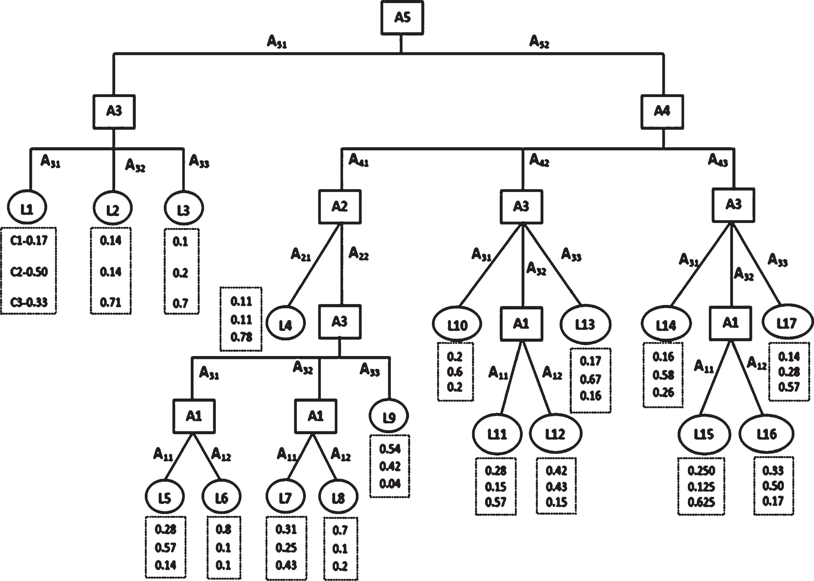
Probability Estimation Decision Tree for 3-class Telecom data.

3.6 Case-3: Applications with ‘n’ number of classes (multi-class) of customers

Often, datasets of business sectors like Telecom, are composed of four, five and more customer classes. In CRM, in one scenario customers are classified as high stay(highest profitable), latent stay, spurious stay, and low stay and in another context, they are classified as stay customers, discount customers, impulsive customers, need based customers, and wandering customers or churn customers(zero profitable) [7]. In the present most challenging scenario of Telecommunications sector to stay alive in their business and for maximizing the profit, most care in various dimensions are being taken. In this business in many instances, customers are categorised as belonging to ‘n’ number of classes and they are arranged in the order of priority in the descending order viz., C₁, C₂, C₃, C₄, ... , C_n based on the amount of profit obtained by them. The intuition is, the amount of profit yielded by the customers will be in the descending order from C₁ to C_n - 1. As the class C_n represents that the customer leaves the enterprise, no profit is expected with respect to this class. Then we try to transform a customer from the undesired/less desirable class to a more desirable class with a maximum net profit.

If a customer is predicted as belonging to an undesired class C_n, then an attempt is made transform him/her to a more desired class among C₁, C₂, ... ,C_n - 1 whichever is more beneficiary to the enterprise. In the n-class scenario, class transformations can be as shown below:

(C_n ⟶ C₁/ C₂/ ... / C_n - 1)

(C_n - 1 ⟶ C₁/ C₂/ ... / C_n - 2)

(n-1). (C₂ ⟶ C₁)

In the case of n-class scenario where n≥2, it is to be noted that, if a customer falls into a leaf node L of the PET, then he/she can likely have the characteristics of all classes. Then except that with respect to class C_n, from all other classes, a customer generates some amount of profit to the enterprise. The total profit obtained from a customer when he/she falls into a leaf node L will be $\sum_{j = 1}^{n - 1} (P_{A_{j}} {* P}_{C_{j}} (L))$ , where P_{A_j} and P_{C_j}(L) are the amount of profit provided to the enterprise if the customer has 1.0 probability of belonging to class-j and probability that the customer belongs to the class-j respectively. For ‘n’ classes of customers (n≥2) profit P obtained from a customer by moving him/her from an undesired/less profitable class to a desired/more profitable one is straight forward and generalized as follows. $\begin{matrix} P & = & \sum_{j = 1}^{n - 1} {(P}_{A_{j}} {* P}_{C_{j}} (D)) - \sum_{j = 1}^{n - 1} {(P}_{A_{j}} {* P}_{C_{j}} (S)) \\ = & \sum_{j = 1}^{n - 1} {(P}_{A_{j}} {* ((P}_{C_{j}} (D)) - P_{C_{j}} (S))) \end{matrix}$ (9)

$Net Profit = \sum_{j = 1}^{n - 1} {(P}_{A_{j}} {* (P}_{C_{j}} (D) - P_{C_{j}} (S))) - \sum_{i} {COST}_{i}$ (10)

In Equation (10), P_{C_j}(D) and P_{C_j}(S) are the probability of class-j in destination and source leaf nodes respectively. Last term in eq. (10) is the total cost incurred on all actions for transforming an instance from source leaf to destination leaf. According to the procedure discussed above, for computing profit in the case of multi-class problems, a method is presented in Algorithm 5.

Algorithm 5

Finding profit for n-class applications where n≥2.
/* S-Source Leaf, D_i - i^th Destination Leaf */
find_profit(S, D_i)
{
P = 0;
for j = 1 to n-1 do
{
P = P+(P_{A_j}* (P_{C_j}(D_i) - P_{C_j}(S)))
}
return (P);
}

4 Performance evaluation and experimental results

In this section, first, the performance of our proposed algorithm is analyzed and then the computational time is verified on various benchmark datasets and a real world Telecom dataset. Then, the run time comparison of our method with the other state-of-the-art methods is performed.

4.1 Performance of ‘Dest_leaf_finder’ algorithm

Computational complexity of ‘Dest_leaf_finder’ algorithm is determined by the number of primitive operations i.e. comparison operations. This algorithm, for each internal node, needs to compare with maximum ‘a’ number of (‘a’ is total number of attributes in the dataset) attributes to identify that attribute. After the attribute identification, to find that attribute’s value, ‘v’ number of comparisons required where ‘v’ is the average number of outcomes of each attribute. Therefore, (a + v) comparisons required up to this stage. If each path contains on average ‘q’ nodes, then total number of comparisons will be (q(a + v)). If the potential destination leaf nodes are ‘p’ then (pq(a + v)) comparisons are needed to find optimal destination leaf node for an instance which has fallen in an undesired leaf. If the total number of instances where we need to find the destination leaf is ‘t’ then (tpq(a + v)) comparisons are required. Eventually, execution time is O(tpq(a + v)).

4.1.1 Experimental setup

During all the experiments discussed in this section, we have implemented the proposed method Dest_leaf_finder in Java programming language and the experiments are conducted on a dual core Pentium 4, 2.5 GHz processor with 4GB RAM running with Windows7 Operating System. Weka source code (Java) has been used for tree construction. All continuous attributes in the datasets are discretized using the Fayyad & Irani’s MDL method [9]. Before applying our proposed postprocessing algorithm on the classifier, we have also evaluated the classifier’s performance by using precision, recall, accuracy, and F-measure. The constructed classifier is tested using 10-fold cross-validation. For evaluating PET’s probability estimation capability, AUC measure is used [15, 19].

We first perform experiments on UCI data and present the scalability feature of our method. Then, the proposed method is compared with the ensemble tree based state-of-the-art methods followed by single tree based state-of-the-art methods. Then, we also verify the performance of our method on the other decision tree construction algorithms. In the end, we focus and demonstrate the time efficiency of our method on the case study problem of the real world Telecom sector.

4.1.2 Statistical test setup

For comparing the performance of the proposed postprocessing method against the state-of-the-art methods, and also to compare the performance of the classifier adopted in our research with other classifiers, we have performed the statistical tests using the popular web statistical tool named STAC (http://tec.citius.usc.es/stac/) [37]. According to the characteristics of the data and as suggested by the online tool, the nonparametric test named Friedman aligned ranks test is performed. In all the experiments in the subsequent sections, the null hypothesis (H₀) for Ranking [11 , 33] is that the means of the results of two or more algorithms are the same. The null hypothesis (H₀) for Post-hoc multiple comparisons [3 , 23] is the mean of the results of each pair of groups is equal.

4.2 Analysis with UCI ML data

The efficiency of our algorithm is verified on ten UCI Machine Learning datasets. The datasets pertaining to classification are taken from UCI ML repository [2] with different number of classes. We have used the Weka (version of 3.8) source code in Java for the Tree construction. Then, we have implemented our algorithm i.e. Dest_leaf_finder in Java programming language.

For each dataset, classes are supposed to have the priority from least to high and tried to convert the instances from low priority class to a higher level priority class such that net profit obtained is maximum. According to attribute’s nature, few of them are assumed as changeable and the remaining as unchangeable. We assumed the classes in the descending order of amount of profit and computed the net profit. The details of UCI datasets which are used in the experiments are shown in Table 5.Technical evaluation measures of the PET constructed on each dataset by using C4.4 algorithm, size of the tree, and the number of leaf nodes of each tree constructed on a dataset also shown in Table 5. The reason for taking these datasets is, they have the sufficient number of records and supporting with n-class data.

Table 5
UCI datasets used in the experiments and technical evaluation measures of C4.4 on the datasets

Dataset No. of instances No. of attributes No. of classes Tree size No. of leaves Precision Recall F-measure Accuracy AUC

Anneal 898 39 6 346 306 0.941 0.942 0.941 94.20 0.965

Autos 205 26 7 215 194 0.854 0.854 0.853 85.37 0.913

Balance Scale 625 4 3 221 199 0.642 0.693 0.666 69.28 0.755

Connect-4 67557 42 3 15952 10635 0.795 0.795 0.795 79.45 0.907

German 1000 20 2 699 599 0.678 0.686 0.681 68.6 0.697

Glass 214 10 7 221 199 0.556 0.579 0.562 57.94 0.775

Heart-c 303 14 5 200 171 0.770 0.769 0.767 76.89 0.835

Hypothyroid 3772 30 4 570 467 0.891 0.923 0.906 92.33 0.818

Nursery 12960 8 5 944 680 0.988 0.988 0.988 98.78 0.999

Solar 1066 12 6 192 145 0.727 0.738 0.729 73.82 0.924

Dataset	No. of instances	No. of attributes	No. of classes	Tree size	No. of leaves	Precision	Recall	F-measure	Accuracy	AUC
Anneal	898	39	6	346	306	0.941	0.942	0.941	94.20	0.965
Autos	205	26	7	215	194	0.854	0.854	0.853	85.37	0.913
Balance Scale	625	4	3	221	199	0.642	0.693	0.666	69.28	0.755
Connect-4	67557	42	3	15952	10635	0.795	0.795	0.795	79.45	0.907
German	1000	20	2	699	599	0.678	0.686	0.681	68.6	0.697
Glass	214	10	7	221	199	0.556	0.579	0.562	57.94	0.775
Heart-c	303	14	5	200	171	0.770	0.769	0.767	76.89	0.835
Hypothyroid	3772	30	4	570	467	0.891	0.923	0.906	92.33	0.818
Nursery	12960	8	5	944	680	0.988	0.988	0.988	98.78	0.999
Solar	1066	12	6	192	145	0.727	0.738	0.729	73.82	0.924

We perceived these datasets as the business data and during the calculation of net profit, in case of a 2-class problem, if an instance has 1.0 probability of belonging to class Non-churn, then profit of $1000 is assumed. Costs of actions are taken in the range $[0–200]. When handling the multi-class datasets, profit obtained when an instance purely belongs to class C₁ and C_n are taken as $1000 and $0 respectively. If there are n classes of instances and if an instance falls into a leaf node representing class-k (k > 1 and k < n) with 1.0 probability, then we have taken a profit of $(1000/k). However, w.r.t. class C_n a profit of $0 is assumed.

From each dataset, each time we have randomly taken a significant amount of examples so as to verify the runtimes of the method. The graphs showed in Fig. 9 presents the run time behavior of the algorithm on 10 UCI datasets. In each graph, x-axis represents the number of instances taken from a dataset and y-axis represents total execution time to find best destination leaf node for each of those instances with a maximum net profit. All the graphs shown in Fig. 9(a) through 9(j) describe running time of Dest_leaf_finder. When tree size is large and it contains a huge number of leaf nodes, run times of Dest_leaf_finder increases since more number of comparisons have to be done to achieve the objective. This fact is observed on the runtimes on the datasets Connect-4 and Hypothyroid.

Fig.9

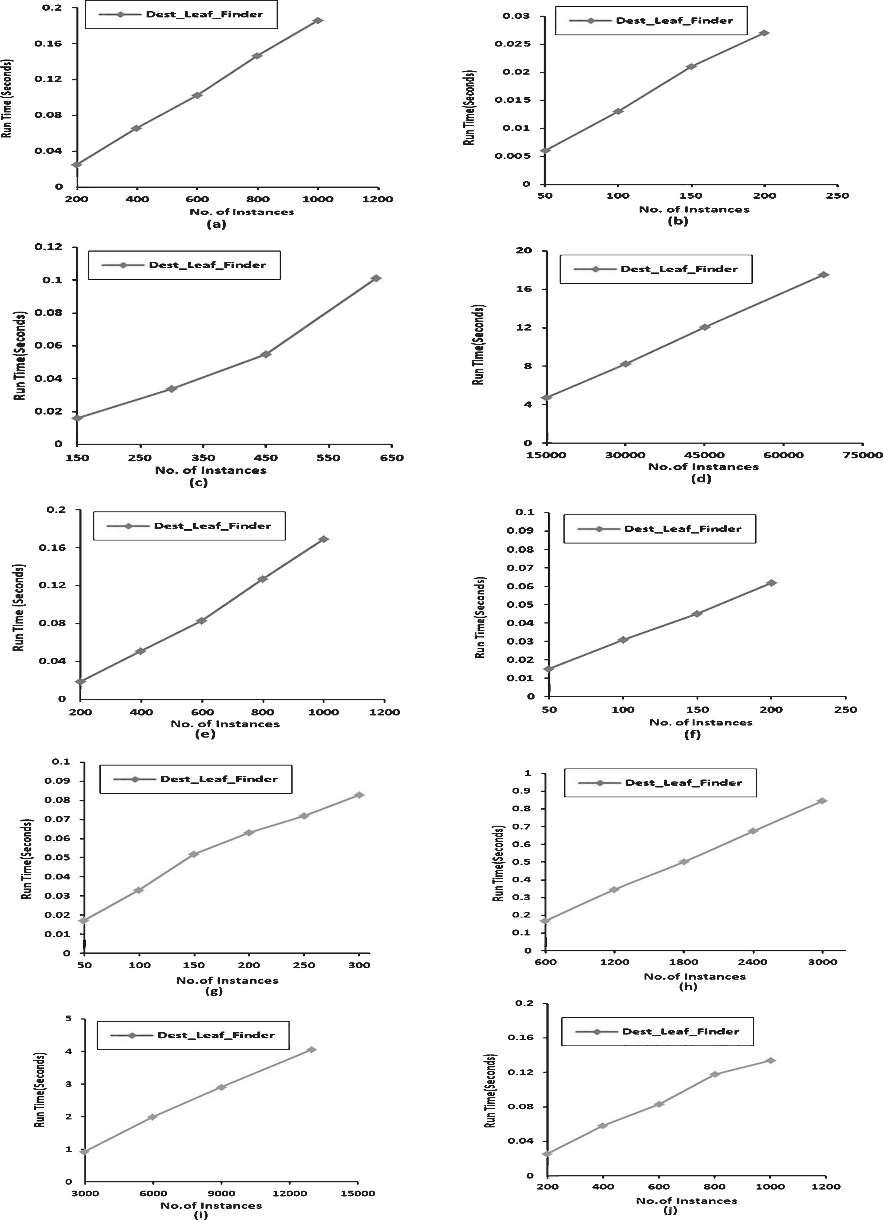
Run Times of Dest_leaf_finder on UCI datasets. (a) Anneal (b) Autos (c) Balance Scale (d) Connect-4 (e) German (f) Glass(g) Heart-c (h) Hypothyroid (i) Nursery (j) Solar.

With the help of our experimental results on UCI ML datasets, it can be concluded that the proposed algorithm, for all kinds of datasets, the running time to achieve the objective function is increasing linearly with the increase of data size and exhibiting the scalability.

4.3 Comparison with ensemble tree based state-of-the-art methods

For comparison, we consider two state-of-the-art techniques viz., Integer Linear Programming (ILP) method [49] and Sub-optimal search algorithm [32], which determines a set of actions that can transform the input instance’s class from undesirable status to desirable. To the best of our knowledge, these are the state-of-the-art ensemble tree based methods for extracting profitable actions. These algorithms mine the best actionable plans from additive tree Model (ATM). Run times of our Dest_leaf_finder algorithm are compared with ILP and Sub-optimal search algorithm on 9 benchmark datasets from the UCI Machine Learning repository and the LibSVM website [51] used in sub-optimal search’s and ILP’s actual experiments. To compare with these state-of-the-art methods, from each dataset we have randomly taken 30 instances from the dataset and produced 30 problems with the same parameter settings. For each dataset, we solve these 30 problems and record the average run time to output the solution. The prime intention of our Dest_leaf_finder is finding the best destination leaf(with maximum net profit) for an input instance which possess undesirable class. By considering all possible solutions and required action costs, Dest_leaf_finder suggests the best destination leaf with an utmost net profit. Hence, we look into the comparison of runtimes of the methods for finding the solution.

Table 6 presents a clear comparison of our Dest_leaf_finder and the two state-of-the-art methods viz. Integer Linear Programming (ILP) and Sub-optimal search algorithm in terms of the runtime for finding the solution. On average Dest_leaf_finder run time is 35.14×10^-3 % of Sub-optimal search algorithm and 16.35×10^–3 % of ILP. In all observations, Dest_leaf_finder execution time is significantly less than those of Sub-optimal search and ILP particularly for the datasets Liver disorders (53.3×10^–5 % and 30×10^–5 %), Australian (2.15×10^–5 % and 3.7×10^–5 %), Breast cancer (260×10^–5 % and 12×10^–5 %). When dataset contains more attributes, Dest_leaf_finder run time is slightly more and however much less than Sub-optimal search algorithm and ILP. This can be observed in the datasets A1a (11083×10^–5 % and 5945.3×10^–5 %), DNA(8501×10^–5 % and 1076×10^–5 %) and Mushrooms (10355×10^–5 % and 7198×10^–5 %).

Table 6
Comparison results of proposed method and two state-of-the-art ensemble tree based algorithms on nine benchmark datasets

Dataset No. of instances No. of attributes No. of classes Accuracy AUC Run time (seconds) $\frac{T 3}{T 1}$ (%) $\frac{T 3}{T 2}$ (%)

ILP (T1) Sub-optimal search algorithm (T2) Dest_leaf_finder (T3)

A1a 32561 123 2 84.38 0.851 7.55 4.05 0.448873 0.059453 0.11083

Australian 690 14 2 85.65 0.891 108.01 1.88 0.004045 0.000037 0.00215

Breast cancer 683 10 2 94.99 0.955 31.04 1.45 0.003771 0.00012 0.00260

DNA 3386 180 3 92.84 0.946 35.47 4.49 0.381717 0.01076 0.08501

Heart 270 13 2 81.85 0.844 5.77 2.31 0.013956 0.00241 0.00604

Ionosphere 351 34 2 89.17 0.923 48.84 2.87 0.010827 0.00022 0.00131

Liver disorders 345 6 2 63.18 0.559 31.62 0.17 0.000091 0.000003 0.00053

Mushrooms 8124 22 2 100.00 1.000 3.87 2.69 0.278563 0.07198 0.10355

Vowel 990 12 11 81.51 0.950 68.73 1.97 0.008292 0.00214 0.00421

Total 46014 502 28 85.95 0.8798 340.9 21.88 1.150135 0.01635 0.03514

(Average) (Average) (Average) (Average)

Dataset	No. of instances	No. of attributes	No. of classes	Accuracy	AUC	Run time (seconds)	$\frac{T 3}{T 1}$ (%)	$\frac{T 3}{T 2}$ (%)
A1a	32561	123	2	84.38	0.851	7.55	4.05	0.448873	0.059453	0.11083
Australian	690	14	2	85.65	0.891	108.01	1.88	0.004045	0.000037	0.00215
Breast cancer	683	10	2	94.99	0.955	31.04	1.45	0.003771	0.00012	0.00260
DNA	3386	180	3	92.84	0.946	35.47	4.49	0.381717	0.01076	0.08501
Heart	270	13	2	81.85	0.844	5.77	2.31	0.013956	0.00241	0.00604
Ionosphere	351	34	2	89.17	0.923	48.84	2.87	0.010827	0.00022	0.00131
Liver disorders	345	6	2	63.18	0.559	31.62	0.17	0.000091	0.000003	0.00053
Mushrooms	8124	22	2	100.00	1.000	3.87	2.69	0.278563	0.07198	0.10355
Vowel	990	12	11	81.51	0.950	68.73	1.97	0.008292	0.00214	0.00421
Total	46014	502	28	85.95	0.8798	340.9	21.88	1.150135	0.01635	0.03514
				(Average)	(Average)				(Average)	(Average)

ILP and Sub-optimal search are employing the ensemble of trees for postprocessing. Postprocessing ensemble of trees obviously requires more computational time.

4.3.1 Statistical test

To compare the performance of Dest_leaf_finder(T3) with Sub-optimal search(T2) algorithm and ILP(T1), statistical tests are performed using the online statistical tool named STAC [37] on the run times given in Table 6. For the experimental results shown in Table 6 where the number of groups k = 3, number of samples n = 9, paired data, the normality condition is not satisfied, but the condition of homoscedasticity is satisfied. Hence, according to the characteristics of the data and as suggested by the online tool the nonparametric test namedFriedman aligned ranks test is performed. For Ranking [11 , 33], the established null hypothesis (H₀): “the means of the results of two or more algorithms are the same”. From the statistical test results furnished in Table 7, the null hypothesis (H₀) has been rejected since the p-value is 0.00106 which is less than the level of significance 0.05. As can be seen from the results in Table 7, it can also be interpreted that there is a significant difference among the mean runtimes and Dest_leaf_finder got the highest rank. For Post-hoc multiple comparison [3 , 23], the null hypothesis (H₀): “the mean of the results of each pair of groups is equal”. In Pairwise comparison, Dest_leaf_finder is significantly different from ILP. Hence, it can be concluded that the proposed method is best among the compared methods with respect to run time.

Table 7
Results of Friedman aligned ranks test on run times in Table 6

Friedman Aligned Ranks test (significance level:0.05)

Proposed method Compared methods Statistic p-value Test result Inference Ranking Post-hoc multiple comparison

Algorithm Rank (Order) Comparing pairs Statistic Adjusted p-value Test result Inference

Dest_leaf_finder (T3) ILP(T1) 13.70222 0.00106 (<0.05) H₀ is rejected Difference is significant T3 8.33333 (1) T3 vs T1 3.91983 0.00027 (<0.05) H₀ is rejected Difference is significant

Sub-optimal search (T2) T2 10.66667 (2) T2 vs T1 3.29622 0.00294 (<0.05) H₀ is rejected Difference is significant

T1 23.00000 (3) T2 vs T3 0.62361 1.00000 (>0.05) H₀ is accepted Difference is not significant

Friedman Aligned Ranks test (significance level:0.05)
Proposed method	Compared methods	Statistic	p-value	Test result	Inference	Ranking	Post-hoc multiple comparison
						Algorithm	Rank (Order)	Comparing pairs	Statistic	Adjusted p-value	Test result	Inference
Dest_leaf_finder (T3)	ILP(T1)	13.70222	0.00106 (<0.05)	H₀ is rejected	Difference is significant	T3	8.33333 (1)	T3 vs T1	3.91983	0.00027 (<0.05)	H₀ is rejected	Difference is significant
	Sub-optimal search (T2)					T2	10.66667 (2)	T2 vs T1	3.29622	0.00294 (<0.05)	H₀ is rejected	Difference is significant
						T1	23.00000 (3)	T2 vs T3	0.62361	1.00000 (>0.05)	H₀ is accepted	Difference is not significant

4.4 Comparison with single tree based state-of-the-art methods

Yang proposed Leaf_Node_Search algorithm [34], a single decision tree based method, to extract actionable knowledge. Kalanat et al. presented F-CEAMA [28] and OF-CEAMA [27] methods for mining actionable knowledge from a single fuzzy decision tree. To our knowledge, these are the state-of-the-art single tree based methods for mining actionable knowledge. Hence, we have compared the performance of our method with them.

For all these methods i.e. Yang’s method, F-CEAMA, OF-CEAMA, and our Dest_leaf_finder, costs of actions are taken in the range $[0–100]. A profit of $1000 is considered, for a customer’s sample, if the probability of belonging to class C₁ is 1.0. Experiments are conducted on the original experimental setup as was done by Kalanat [27, 28].

The methods are implemented in Java programming language and the experiments are conducted on a dual core Pentium 4, 2.5 GHz processor with 4GB RAM running with Windows7 Operating System. Experiments are conducted on UCI datasets which are shown in Table 8. All these datasets, except Australian, are imbalanced where majority instances are labelled with ‘Non-churn/Positive’ class. Therefore, from each dataset, instances are randomly selected such that numbers of positive and negative/Churn instances are equal. As Kalanat’s methods [27, 28] use a fuzzy method, their methods’ performance is significant on numeric attributes only. Hence, the datasets are used in two ways. In the first version, we have taken all types i.e. numeric andcategorical attributes(N&C) and in the second version, only numeric attributes(N) from the datasets are taken and conducted the experiments. In these experiments, we have not considered comparing the profits obtained after changing the instance from one leaf to another.

Table 8
UCI Datasets used in the experiments for run time comparison with single tree based state-of-the-art methods

Dataset Total no. of attributes No. of numerical attributes No. of instances No. of negative/Churn instances

Australian Credit Approval 15 6 690 383

German Credit Approval 20 7 1000 700

German-Numerical Credit Approval 25 25 1000 700

Adult 15 6 10000 7621

Dataset	Total no. of attributes	No. of numerical attributes	No. of instances	No. of negative/Churn instances
Australian Credit Approval	15	6	690	383
German Credit Approval	20	7	1000	700
German-Numerical Credit Approval	25	25	1000	700
Adult	15	6	10000	7621

The reason is, our method extensively searches all possibilities and eventually outputs only the optimal solution with maximum net profit without leaving any best option which is also illustrated in sections 3.4 and 3.5. The constructed classifier is tested using 10-fold cross validation.

F-CEAMA works with an assumption that all attributes are flexible (whose values are possible to change). On the other hand, OF-CEAMA, Dest_leaf_finder, and Yang’s method considers the reality and separates the attributes as flexible and non-flexible. Experimental results shown in Table 9 describes that when compared with these three methods Dest_leaf_finder exhibits better computational performance. We have presented the run times of our method in both cases i.e. treating all attributes as flexible and only the selected attributes as flexible. When all attributes are flexible, then runtime of Dest_leaf_finder slightly increases since each path from the root to the leaf node has to be fully processed. If the average length of the paths from the root to a leaf node is ‘len’, then, for every path ‘len’ number of comparisons have to be performed. In the other scenario, we only try to change the values of required flexible attributes. In this case, along a path, if a non-flexible attribute is encountered and its value is required to change, then that path is ignored and comparing the values of remaining attributes’ values along that path is not performed. The reason why the run times of F-CEAMA and OF-CEAMA are more than that of Dest_leaf_finder is since their search space is more. This is because, for an instance, F-CEAMA considers multiple source leaf nodes whereas Yang’s method, and our Dest_leaf_finder considers only one source leaf for an instance. Yang’s method considers a large number of candidate actions that leads to more computational complexity when compared to our method. Out of all the attributes, when only numeric attributes are taken from the dataset, then the tree size and number of leaf nodes decrease. Then, Dest_leaf_finder’s runtime decreases accordingly. On the other hand, in the same scenario, the other methods computational time is not decreasing since; the fuzzy concept is appropriate for numeric attributes and they apply the fuzzy approach in every phase of finding fuzzy net profit. Above all, Dest_leaf_finder’s approach is different since it works for multi-class applications whereas the other methods deal the problem as 2-class only.

Table 9

Run Time comparison results of Dest_leaf_finder and other single tree based state-of-the-art methods

Dataset	Types of attributes included in experiments	Run time (seconds)
		Yang’s method (All attributes are Flexible)	F-CEAMA	OF-CEAMA	Dest_Leaf_Finder (All attributes are Flexible)	Dest_leaf_finder (Only selected attributes are Flexible)
Australian	N&C	0.169	0.169	0.169	0.029	0.026
Australian	N	0.647	0.795	0.796	0.0356	0.0315
German	N&C	0.744	0.88	0.89	0.142	0.129
German	N	0.901	1.202	1.274	0.066	0.061
German-numerical	N	0.589	1.532	1.539	0.243	0.231
Adult	N&C	2.7	2.7	3.2	0.481	0.465
Adult	N	1.692	2.4	3.9	0.032	0.030

4.4.1 Statistical test

In order to statistically analyze the performance of Dest_leaf_finder with other class of state-of-the-art profit maximizing postprocessing methods based on a single tree viz., Yang’s method, F-CEAMA, and OF-CEAMA tests are performed using STAC on the run times given in Table 9. For the experimental results shown in Table 9 the number of groups k = 5, the number of samples n = 7, paired data where normality has not satisfied and homoscedasticity satisfied. Hence, according to the characteristics of the data and as suggested by the online tool the nonparametric test named Friedman aligned ranks test is performed. From the results furnished in Table 10, it can be interpreted that there is a significant difference among the mean runtimes and the proposed methods implemented in two ways i.e. Dest_leaf_finder(Only) where only numeric attributes are taken and Dest_leaf_finder (all) i.e. all attributes in the dataset are taken got the highest ranks. Post-hoc multiple comparison results also prove that Dest_leaf_finder is significantly different from F-CEAMA, and OF-CEAMA. Therefore, we can say that the proposed method outperforms the compared methods with respect to runtime.

Table 10
Results of Friedman aligned ranks test on data in Table 9

Friedman Aligned Ranks test (significance level:0.05)

Proposed method Compared method Statistic p-value Test result Inference Ranking Post-hoc multiple comparison

Algorithm Rank (Order) Comparing pairs Statistic Adjusted p-value Test result Inference

Dest_leaf_finder (Only) Yang’s method 0.00023 0.00023 (<0.05) H₀ is rejected Difference is significant Dest_leaf_finder (Only) 7.00000 (1) Dest_leaf_finder (Only) Vs OF-CEAMA 3.78189 0.00156 H₀ is rejected Difference is significant

OF-CEAMA Vs Dest_leaf_finder (All) 3.54716 0.00389 H₀ is rejected Difference is significant

F-CEAMA Dest_leaf_finder (All) 8.28571 (2) Dest_leaf_finder (Only) Vs F-CEAMA 3.53411 0.00409 H₀ is rejected Difference is significant

F-CEAMA Vs Dest_leaf_finder (All) 3.29938 0.00969 H₀ is rejected Difference is significant

Dest_leaf_finder (All) Yang’s method 20.64286 (3) Dest_leaf_finder (Only) Vs Yang’s method 2.49083 0.12744 H₀ is accepted Difference is significant

Dest_leaf_finder (All) Vs Yang’s method 2.25610 0.24065 H₀ is accepted Difference is significant

OF-CEAMA F-CEAMA 26.35714 (4) OF-CEAMA Vs Yang’s method 1.29106 1.00000 H₀ is accepted Difference is not significant

F-CEAMA Vs Yang’s method 1.04328 1.00000 H₀ is accepted Difference is not significant

OF-CEAMA 27.71429 (5) OF-CEAMA Vs F-CEAMA 0.24778 1.00000 H₀ is accepted Difference is not significant

Dest_leaf_finder (Only) Vs Dest_leaf_finder (All) 0.23474 1.00000 H0 is accepted Difference is not significant

Friedman Aligned Ranks test (significance level:0.05)
Dest_leaf_finder (Only)	Yang’s method	0.00023	0.00023 (<0.05)	H₀ is rejected	Difference is significant	Dest_leaf_finder (Only)	7.00000 (1)	Dest_leaf_finder (Only) Vs OF-CEAMA	3.78189	0.00156	H₀ is rejected	Difference is significant
								OF-CEAMA Vs Dest_leaf_finder (All)	3.54716	0.00389	H₀ is rejected	Difference is significant
	F-CEAMA					Dest_leaf_finder (All)	8.28571 (2)	Dest_leaf_finder (Only) Vs F-CEAMA	3.53411	0.00409	H₀ is rejected	Difference is significant
								F-CEAMA Vs Dest_leaf_finder (All)	3.29938	0.00969	H₀ is rejected	Difference is significant
Dest_leaf_finder (All)						Yang’s method	20.64286 (3)	Dest_leaf_finder (Only) Vs Yang’s method	2.49083	0.12744	H₀ is accepted	Difference is significant
								Dest_leaf_finder (All) Vs Yang’s method	2.25610	0.24065	H₀ is accepted	Difference is significant
	OF-CEAMA					F-CEAMA	26.35714 (4)	OF-CEAMA Vs Yang’s method	1.29106	1.00000	H₀ is accepted	Difference is not significant
								F-CEAMA Vs Yang’s method	1.04328	1.00000	H₀ is accepted	Difference is not significant
						OF-CEAMA	27.71429 (5)	OF-CEAMA Vs F-CEAMA	0.24778	1.00000	H₀ is accepted	Difference is not significant
								Dest_leaf_finder (Only) Vs Dest_leaf_finder (All)	0.23474	1.00000	H0 is accepted	Difference is not significant

4.5 Performance comparison of Dest_leaf_finder on other Decision tree algorithms

To verify the performance of our method on other decision tree construction algorithms, we have used two other standard decision tree construction algorithms viz. Random Tree and Decision stump. Our method is based on a single decision tree. The reason for using these algorithms is, they also generate a single decision tree and the Random Tree algorithm generates a large tree and Decision stump generates a very short tree. Hence, our method can be best compared with the help of these two decision tree construction algorithms. Random Tree algorithm has been introduced by Leo Breiman. During the tree construction, this algorithm finds the best splitting attribute at each node among the randomly chosen subset of attributes. On the other hand, Decision stump [44] algorithm produces a decision tree with only one level and outputs class label of an instance based on a single attribute. For comparison, we have used the dataset in Table 2. Figures 10(a), 10(b) and 10(c) show the PETs constructed using C4.4, Decision stump, and Random Tree respectively on the dataset in Table 2. Table 11 compares the run times and net profits of Dest_leaf_finder on various decision tree construction algorithms on the Telecom sample dataset shown inTable 2.

Fig.10

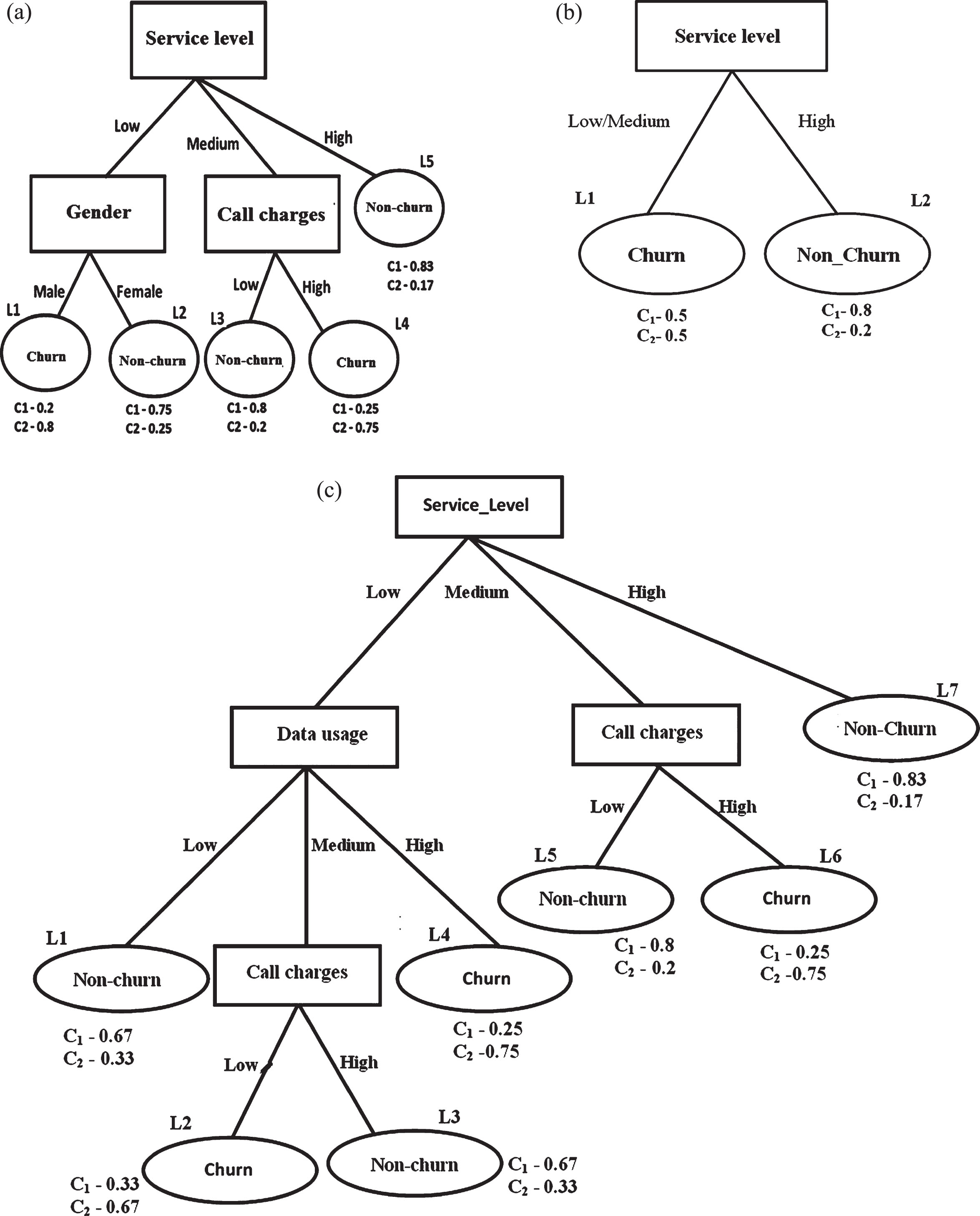
(a) PET constructed using C4.4. (b) PET constructed using Decision stump. (c) PET constructed using Random Tree.

Table 11

Performance comparison of Dest_leaf_finder on the trees constructed using various Classifiers on Telecom dataset in Table 2

Decision Tree algorithm	Source leaf node	Class label	Class-C₁ probability	Class-C₂ probability	Destination leaf	Net Profit($) for one sample X	Net Profit($) for the total dataset	Run Time (seconds)
C4.4	L1	Churn	0.2	0.8	L3	500	2390	0.000047
Random Tree	L4	Churn	0.25	0.75	L5	450	2100	0.000076
Decision stump	L1	Churn	0.5	0.5	L2	100	700	0.000011

If an instance has 1.0 probability of belonging to class Non-churn, then profit of $1000 is considered. Cost matrices which are shown in Fig. 5 areused.

Details of the trees constructed using various methods on Table 2 along with their technical evaluation measures are shown in Table 12. As can be seen from Table 12, accuracy and AUC values of Decision stump method are not up to the mark. To differentiate the three methods, a sample X from the dataset in Table 2 has been taken and net profits, when our Dest_leaf_finder is applied on the three trees built using the three methods have been computed. X=Service_Level = Low, Data usage = High, Gender = Male, Call charges = Low. For this sample, C4.4 produced a maximum net profit($500) when compared with the other two methods ($450 and $100). The reason is, C4.4 produced a balanced decision tree with size 8 and 5 leaf nodes.

Table 12

Details of PETs constructed on Telecom dataset (Table 2) using various classifiers

Decision Tree construction algorithm	Tree size	No. of leaves	Accuracy	AUC

C4.4	8	5	1.000	1.000
Random Tree	11	7	1.000	1.000
Decision stump	3	2	0.6428	0.722

On the other hand, Random Tree generates relatively large decision tree with more number of leaf nodes. If the height of the tree is more, then there is a possibility of making more attribute value changes which eventually leads to more cost and thereby leads to a reduction in net profit. For performing more number of comparisons and actions it also takes more runtime. Hence, the run time of our Dest_leaf_finder increases when the tree is built using Random Tree method. When the tree is built using Decision stump, a very short tree with only one level is obtained every time. But, the technical interestingness measures of the Decision stump are not in the acceptablerange.

However, as always a single comparison is to be performed, computation time can be very less with Decision stump. The other drawback when the tree is built using Decision stump is, the objective of obtaining maximum net profit does not fulfil. The reason is, always there will be only one possible destination leaf for an instance which has fallen into an undesired leaf node. The total net profit obtained for all the instances (labelled with class ‘Churn’) from the dataset in Table 2 by postprocessing the trees built using C4.4, Random Tree, and Decision stump are $2390, $2100, and $700 respectively where C4.4 is yielding maximum.

Experiments also conducted on10 UCI datasets to verify the performance of Dest_leaf_finder on three decision tree algorithms. Table 13 compares the run times on three decision tree construction algorithms. Same profit values and action costs are employed as discussed in Section 4.2. For each dataset, trees are built using the three decision tree methods. For each instance in a dataset, a destination leaf node with a maximum net profit is computed on each tree separately. Such a way computational time for all the instances in each of the 10 UCI datasets is recorded on three trees. It has been observed that Decision stump is outperforming the other two. But the Decision stump’s technical evaluation measures are poor on all the datasets as proven in the following statistical analysis.

Table 13

Run time comparison of ‘Dest_leaf_finder ’ on three Decision Tree construction algorithms on UCI data

Dataset	Run time (seconds)
	C4.4	Random Tree	Decision stump
Anneal	0.1859	1.7804	0.000592
Autos	0.027	0.067	0.000137
Balance Scale	0.101	1.473	0.000411
Connect-4	17.503	106.732	0.03824
German	0.169	0.609	0.000648
Glass	0.062	0.255	0.000139
Heart-c	0.083	0.318	0.000164
Hypothyroid	0.846	8.902	0.001911
Nursery	4.055	11.034	0.007842
Solar	0.1342	0.326	0.000683
Telecom (Sample data)	0.000047	0.00007	0.000011

4.5.1 Statistical test

To compare the runtime performance of the classification model constructed using C4.4 against the models built using Random Tree and Decision stump statistical tests are performed using STAC on the data in Table 13. For the given data in Table 13, the number of groups k = 3, number of samples n = 11, paired data where normality is not satisfied and homoscedasticity satisfied. Hence, according to the characteristics of the data and as suggested by the online tool the non-parametric test named Friedman aligned ranks test is applied. From the results shown in Table 14, it can be interpreted that there is a significant difference among the mean runtimes and Decision stump got the highest rank followed by C4.4. In Pairwise comparison, C4.4 is significantly different from Random Tree but has no significant difference from Decision stump.

Table 14
Results of Friedman aligned ranks test on data in Table 13

Friedman Aligned Ranks test (significance level:0.05)

Adopted Classifier Compared Classifier Statistic p-value Test result Inference Ranking Post-hoc multiple comparison

Classifier Rank (Order) Comparing pairs Statistic Adjusted p-value Test result Inference

C4.4 Random Tree 16.68638 0.00024 (<0.05) H₀ is rejected Difference is significant Decision stump 10.18182 (1) Decision stump vs Random Trees 4.32154 0.00005 H₀ is rejected Difference is significant

Decision stump C4.4 12.81818 (2) Random Trees vs C4.4 3.68213 0.00069 H₀ is rejected Difference is significant

Random Tree 28.00000 (3) Decision stump vs C4.4 0.63941 1.00000 H₀ is accepted Difference is not significant

Friedman Aligned Ranks test (significance level:0.05)
Adopted Classifier	Compared Classifier	Statistic	p-value	Test result	Inference	Ranking	Post-hoc multiple comparison
						Classifier	Rank (Order)	Comparing pairs	Statistic	Adjusted p-value	Test result	Inference
C4.4	Random Tree	16.68638	0.00024 (<0.05)	H₀ is rejected	Difference is significant	Decision stump	10.18182 (1)	Decision stump vs Random Trees	4.32154	0.00005	H₀ is rejected	Difference is significant
	Decision stump					C4.4	12.81818 (2)	Random Trees vs C4.4	3.68213	0.00069	H₀ is rejected	Difference is significant
						Random Tree	28.00000 (3)	Decision stump vs C4.4	0.63941	1.00000	H₀ is accepted	Difference is not significant

Complete technical evaluation measures of three decision tree algorithms are presented in Tables 15, 16, and 17. These results also depict that C4.4 exhibits better performance in all aspects. However, it can be observed from Table 17 that the accuracy and AUC measures of Decision stump are not in the acceptable range on many datasets. For Decision stump, average accuracy and AUC values are 64.38 and 0.6791 respectively which are not up to the mark.

Table 15

Technical evaluation measures of C4.4 on UCI datasets

Dataset	Tree Size	#Leaves	Precision	Recall	F-measure	Accuracy	AUC
Anneal	346	306	0.941	0.942	0.941	94.20	0.965
Autos	215	194	0.854	0.854	0.853	85.37	0.913
Balance Scale	221	199	0.642	0.693	0.666	69.28	0.755
Connect-4	15952	10635	0.795	0.795	0.795	79.45	0.907
German	699	599	0.678	0.686	0.681	68.6	0.697
Glass	221	199	0.556	0.579	0.562	57.94	0.775
Heart-c	200	171	0.770	0.769	0.767	76.89	0.835
Hypothyroid	570	467	0.891	0.923	0.906	92.33	0.818
Nursery	944	680	0.988	0.988	0.988	98.78	0.999
Solar	192	145	0.727	0.738	0.729	73.82	0.924

Table 16

Technical evaluation measures of Random Tree on UCI datasets

Dataset	Tree Size	#Leaves	Precision	Recall	F-measure	Accuracy	AUC
Anneal	1452	1278	0.893	0.896	0.894	89.64	0.928
Autos	362	334	0.766	0.766	0.766	76.58	0.891
Balance Scale	1031	967	0.639	0.688	0.661	68.8	0.753
Connect-4	78964	1510	0.698	0.697	0.697	69.68	0.721
German	1677	1449	0.683	0.690	0.686	69.00	0.638
Glass	571	518	0.529	0.533	0.525	53.27	0.690
Heart-c	508	446	0.728	0.726	0.722	72.60	0.745
Hypothyroid	3283	2861	0.892	0.918	0.904	91.78	0.679
Nursery	1872	1196	0.947	0.946	0.947	94.62	0.976
Solar	455	322	0.708	0.721	0.710	72.13	0.879

Table 17

Technical evaluation measures of decision stump on UCI datasets

Dataset	Tree size	#Leaves	Precision	Recall	F-measure	Accuracy	AUC
Anneal	4	3	0.744	0.772	0.745	77.17	0.845
Autos	4	3	0.264	0.449	0.333	44.87	0.651
Balance Scale	4	3	0.499	0.541	0.518	54.08	0.575
Connect-4	4	3	0.433	0.658	0.523	65.83	0.567
German	4	3	0.490	0.700	0.576	70.00	0.654
Glass	4	3	0.265	0.472	0.326	47.19	0.605
Heart-c	4	3	0.718	0.716	0.717	71.61	0.680
Hypothyroid	4	3	0.885	0.934	0.909	93.42	0.605
Nursery	4	3	0.496	0.663	0.551	66.25	0.828
Solar	4	3	0.383	0.535	0.421	53.47	0.781

After Decision stump, C4.4 run time performance is fine when compared with Random Tree. Average accuracy and AUC values of C4.4 are 79.666 and 0.8588 which are even better than the values of Random Tree i.e. 75.81 and 0.79.

Table 18 compares the accuracy of three classifiers and Table 19 compares the AUC of three classifiers on 10 UCI datasets.

Table 18

Comparison of Accuracy of three classifiers

Data set	Accuracy
	C4.4	Random Tree	Decision stump
Anneal	94.2	89.64	77.17
Autos	85.37	76.58	44.87
Balance Scale	69.28	68.8	54.08
Connect-4	79.45	69.68	65.83
German	68.6	69	70
Glass	57.94	53.27	47.19
Heart-c	76.89	72.6	71.61
Hypothyroid	92.33	91.78	93.42
Nursery	98.78	94.62	66.25
Solar	73.82	72.13	53.47
Average	79.666	75.81	64.389

Table 19

Comparison of AUC of three Classifiers

Data Set	Accuracy
	C4.4	Random Tree	Decision stump
Anneal	0.965	0.928	0.845
Autos	0.913	0.891	0.651
Balance Scale	0.755	0.753	0.575
Connect-4	0.907	0.721	0.567
German	0.697	0.638	0.654
Glass	0.775	0.69	0.605
Heart-c	0.835	0.745	0.68
Hypothyroid	0.818	0.679	0.605
Nursery	0.999	0.976	0.828
Solar	0.924	0.879	0.781
Average	0.8588	0.79	0.6791

For the statistical analysis of the accuracy and AUC of C4.4 against two other classifiers, we have used the same web platform STAC. For the given data in Tables 18 and 19, the number of groups k = 3, number of samples n = 10, paired data where normality is not satisfied and homoscedasticity not satisfied. Hence, the nonparametric test i.e. Friedman aligned ranks test is performed. The statistical test results presented in Tables 20 and 21 depict that there is a significant difference among the mean accuracy and also among the mean AUC values. Regarding two metrics, C4.4 got the least rank with respect to minimization and therefore provides the highest accuracy and highest AUC. The Post-hoc multiple comparison results in Tables 20 and 21 also describe that in pairwise comparison, C4.4 is significantly different from Decision stump, but not significantly different from Random Tree with respect to accuracy and AUC.

Table 20

Results of Friedman aligned ranks test on Accuracy data in Table 18

Friedman Aligned Ranks test (significance level:0.05)
Adopted classifier	Compared classifier	Statistic	p-value	Test result	Inference	Ranking		Post-hoc multiple comparison
						classifier	rank (order)	comparing pairs	statistic	adjusted p-value	test result	inference
C4.4	Random Tree	11.78988	0.00275 (<0.05)	H₀ is rejected	Difference is significant	Decision stump	6.90000 (3)	Decision stump vs C4.4	3.91160	0.00028	H₀ is rejected	Difference is significant
	Decision stump					Random Trees	17.30000 (2)	Decision stump vs Random Trees	2.64160	0.02475	H₀ is rejected	Difference is significant
						C4.4	22.30000 (1)	Random Trees vs C4.4	1.27000	0.61225	H₀ is accepted	Difference is not significant

Table 21

Results of Friedman aligned ranks test on AUC data in Table 19

Friedman Aligned Ranks test (significance level:0.05)
Adopted Classifier	Compared Classifier	Statistic	p-value	Test result	Inference	Ranking		Post-hoc multiple comparison
			Classifier	Rank (Order)	Comparing pairs	Statistic	Adjusted p-value	Test result	Inference
C4.4	Random Tree	16.17289	0.00031 (<0.05)	H₀ is rejected	Difference is significant	Decision stump	5.80000 (3)	Decision stump Vs C4.4	4.80060	0.00000	H₀ is rejected	Difference is significant
	Decision stump					Random Tree	16.00000 (2)	Decision stump Vs Random Tree	2.59080	0.02873	H₀ is rejected	Difference is significant
						C4.4	24.70000 (1)	Random Tree Vs C4.4	2.20980	0.08136	H₀ is accepted	Difference is not significant

The run time of our Dest_leaf_finder increases when tree size increases. A tree possessing acceptable technical evaluation measures (Accuracy, AUC, etc.) and is shallow with less number of leaf nodes is preferable for our work. The benchmark method C4.4 serves this purpose. It can be concluded that still, C4.4 is the remarkable classifier since its accuracy and AUC are significant and produces reasonably shallower trees which are suitable for the research in this paper.

4.6 Experiments on real Telecom data

We consider the real Telecom dataset whose details are discussed in Section 3.2 for experiments. First, we perform the experiments on the total dataset and show the runtime results. We show that our method is efficient and scalable in this 2-class scenario. Thereafter, we verify the performance of the proposed method on the sample data extracted from the original dataset. Later, to demonstrate the performance of our method on multi-class setting, we also consider the 3-class version of this data and perform the experiments.

4.6.1 Experiments on 2-class real Telecom data

In this section, we verify the performance of our Dest_leaf_finder on the large real time Telecom dataset, whose details are discussed in Section 3.2. Out of the 15000 customers records in this dataset, 2500 are ‘Churn’ and the remaining 12500 are ‘Non-churn’. To avoid imbalanced decision tree thereby predicting most of the customers as ‘Non-churn’, we have randomly sampled 2500 ‘Non-churn’ records out of the 12500 records, and all the 2500 ‘Churn’ records are used. Experiments are performed totally on 5000 records.

A PET is built using C4.4 method. After the PET is constructed, it is tested using 10-fold cross validation method. The constructed PET has 734 leaf nodes. Out of them, 388 represented the class label ‘Churn’ and the remaining 346 represented the class ‘Non-churn’. Costs are taken in the range $[0–200]. If an instance has 1.0 probability of belonging to class Non-churn, then a profit of $1000 is assumed. Then, we applied our Dest_leaf_finder on the constructed PET.

Performance comparison with other Tree construction algorithms on Telecom data: Performance comparison of proposed method is also done on various other tree construction algorithms on the real Telecom dataset. Technical evaluation measures of the PETs constructed on the Telecom dataset on 5000 records using the three decision tree algorithms is presented in Table 22. The results in Table 22 depict that C4.4 shown better results than those of the other two. We have made the comparison of run times by using the three PETs separately. Each time a set of records from the dataset are taken and given as the input to Dest_leaf_finder. For each of these set of records, the proposed algorithm determines optimal destination leaf with maximum net profit on three trees separately. Total runtime for all the records in the set is recorded. Each time we have increased the size of the input data samples. Runtimes of the proposed method on the real Telecom data on different classifiers is presented in Table 23.

Table 22
Technical evaluation measures of various decision tree algorithms on Real Telecom dataset

Decision tree algorithm

C4.4 Random Tree Decision stump

Accuracy AUC Accuracy AUC Accuracy AUC

88.04 0.892 71.33 0.628 60.23 0.601

Decision tree algorithm
C4.4	Random Tree	Decision stump
Accuracy	AUC	Accuracy	AUC	Accuracy	AUC
88.04	0.892	71.33	0.628	60.23	0.601

Table 23

Performance comparison of Dest_leaf_finder on Real Telecom dataset using various Tree construction algorithms

No. of records sampled from Telecom Dataset	Decision tree algorithm Run Time (seconds)
No. of records sampled from Telecom Dataset		C4.4	Random Tree	Decision stump
1000	0.2401	2.117	0.000613
2000	0.4013	3.916	0.001237
3000	0.6197	7.004	0.001745
4000	0.8311	9.283	0.002571
5000	1.1631	13.411	0.003729
Sum	3.2553	35.731	0.009895
Average	0.65106	7.1462	0.001979

From the results shown in Table 23 it has been observed that the proposed method is scalable when it is applied on the tree constructed using C4.4. On the other hand, runtimes of Dest_leaf_finder are increasing more when it is applied on the tree constructed using the Random Tree. Total and average run times of the method when applied on C4.4 is at least ten times less than that of Random forest. Though the Decision stump’s runtime values are better than that of C4.4, it is not considered since its accuracy and AUC values are low. From the results in Table 22, it can be seen that the accuracy and AUC measures of Decision stump are 60.23 and 0.601 which are not in the acceptable range. On the other hand, C4.4 exhibited comprehensive values for accuracy and AUC i.e. 88.04 and 0.892 respectively.

Statistical test: Statistical tests are performed on the run times presented in Table 23 to compare the performance of C4.4 with other classifiers using the STAC platform. For the given data in Table 23, Friedman aligned ranks test is performed since normality not satisfied and homoscedasticity is satisfied. From the results shown in Table 24, it can be interpreted that there is a significant difference among the mean runtimes and Decision stump got the highest rank followed by C4.4. In Pairwise comparison, C4.4 is significantly different from Random Tree but has no significant difference from Decision stump with respect to runtime.

Table 24

Results of Friedman aligned ranks test on data in Table 23

Friedman Aligned Ranks test (significance level:0.05)
Adopted Classifier	Compared Classifier	Statistic	p-value	Test result	Inference	Ranking		Post-hoc multiple comparison
						Classifier	Rank (Order)	Comparing pairs	Statistic	Adjusted p-value	Test result	Inference
C4.4	Random Tree	7.60000	0.02237 (<0.05)	H₀ is rejected	Difference is significant	Decision stump	5.00000	Decision stump Vs Random Tree	2.82843	0.01403	H₀ is rejected	Difference is significant
	Decision stump					C4.4	6.00000	Random Tree Vs C4.4	2.47487	0.03998	H₀ is rejected	Difference is significant
						Random Tree	13.00000	Decision stump Vs C4.4	0.35355	1.00000	H₀ is accepted	Difference is not significant

4.6.2 Experiments on sample 2-class real Telecom data

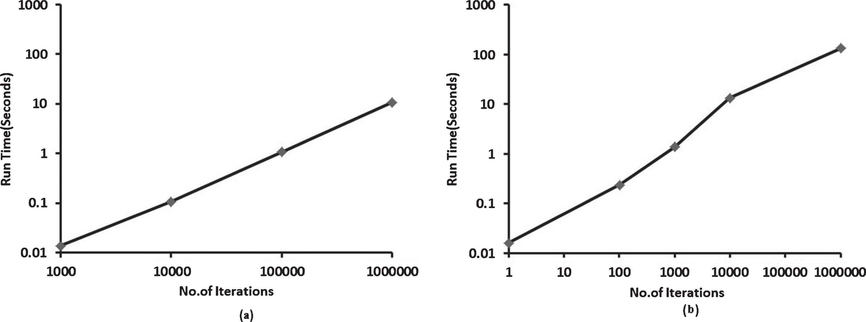
To validate the efficiency of our proposed algorithm, we have performed the experiments on the subset of real Telecom data discussed in Section 3.4. This dataset contains 14 examples as given in Table 2 whose profit value (P_A) and cost matrices details are also discussed in Section 3.4. Experimental results are presented in Fig. 11, where the log scale is used in all the graphs on both x-axis and y-axis and incremented by multiples of 10. For each instance, the run time to find the best destination leaf node with maximum net profit is recorded. For notable observation of the run times of the proposed algorithm, one instance has been randomly taken from the dataset and it is iterated for a large number of times and the run times are recorded. Figure 11(a) depicts the run time of one instance on a different number of iterations with the proposed method. This has been observed for different instances from the dataset and also for a different number of iterations. As the other case, we have taken the entire dataset and noted the execution time on large number of runs. In this case, from the dataset, each time one instance is given as input to Dest_leaf_finder for finding the best solution, and the run time is recorded separately. Such a way, run time is recorded for all the instances of the dataset. This process is repeated for a large number of times on the same dataset to have clear observation. The graph shown in 8(b) depicts that in all the cases, run times are increased linearly with the increase in the size of the dataset. The total net profit obtained after transforming all the ‘Churn’ customers as ‘Non-churn’ is $2390. However, the net profit obtained for each of the customer’s instance is not presented in the experimental results since in all scenarios our method provides a maximum possible value.

Fig.11

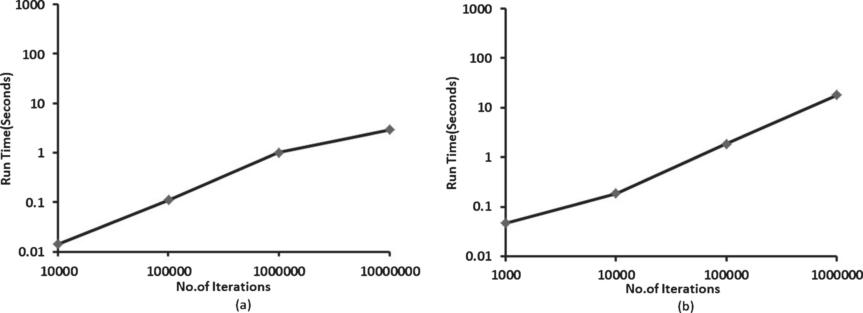
Run Times of Dest_leaf_finder on the sample 2-class Telecom dataset. (a) Single instance of 2-class Telecom data (b) Entire 2-class Telecom data.

4.6.4 Experiments on 3-class scenario of real Telecom data

To explain the working of our proposed method for multi-class setting, we have used the 3-class version of the real Telecom data with 125 customers’ records which is discussed in Section 3.5. In this case, an attempt is made to change ‘Churn customer’ as either ‘Non-churn and active customer’ and if not possible at least as a ‘Non-churn but inactive customer’. However, a ‘Non-churn but inactive customer’ will be converted as a ‘Non-churn and active customer’. This scenario is familiar in the Telecom industry since, a good percentage of customers are not cancelling their subscription, stay with the service provider but inactive in using the services thereby leading to least profits. Profits are considered such that if the customer’s C₁ class probability is 1.0 then profit is $1000, C₂ class probability is 1.0 then profit is $500 according to the expert in the Telecom business. First, one record is taken from the dataset and it is iterated significantly a large number of times and the total run time is noted. Figure 12(a) shows the running times of Dest_leaf_finder for this scenario. Here the observed run times are high as compared with the case observed in Fig. 11(a) where dataset size is 14 and the number of leaf nodes in the tree is 5 only. As the 3-class Telecom dataset contains 125 records, the size of the induced decision tree is large with 17 leaf nodes. Hence, there are 16 possibilities for finding the destination leaf. This is the reason for the increase in the run time as compared with the run times in the case of 2-class dataset in Fig. 11(a).

Fig.12

Run Times of Dest_leaf_finder on the real 3-class Telecom dataset (a) Single instance of Telecom data (b) Entire Telecom dataset.

As another case, we have also iterated this entire dataset significantly large number of times to clearly verify the runtimes. The results are depicted in Fig. 12(b). For the same scenario shown in Fig. 11(b) for the 2-class dataset, the recorded runtimes are low. The reason for the increase in the runtime for Telecom dataset is, in one iteration 125 records are given as input to the large tree whereas in the former case (Fig. 11(b)) 14 records as input to a simple decision tree.

Dest_leaf_finder fits well and it is relevant to the Telecom sector, the industry facing high attrition rate and fall down in profits due to various classes of reluctant customers. When the churning problem of Telecom sector is perceived as a 2-class problem, the work of Dest_leaf_finder is much easier since it tries to find a destination leaf which is labelled with ‘Non-churn’ only. For the other practical case where the customers are treated as belonging to three classes, the proposed method provides optimal profit maximizing solution. It sets most of the existing customers to be in higher desirable classes in this case.

According to circumstances, even if the Telecom customers are classified as belonging to more than three classes based on the profitability, the proposed method can shift the customers from lower profitable classes to higher profitable classes. Eventually, the proposed method’s objective is increasing profits of Telecom sector which is a vital task for it. It can be concluded that for all contexts of the case study problem, proposed method provides maximum possible net profit and its run time efficiency is fine and especially its performance on the C4.4 decision tree is superior. The proposed method provides an efficient solution by reducing the search space in finding the solution and incorporating some of the steps like the early stopping of considering a candidate destination leaf when an unchangeable attribute is encountered along the path of destination leaf. Thus, the proposed method can provide efficient and lucrative solution to the Telecom sector.

5 Conclusions and future work

In the challenging Telecom industry, to support the decision making process, decision makers rely more on various data mining methods since the undesired status of the customers need to be changed to the desired one to acquire more profits. In this paper, we presented a method, suitable for Telecom sector, for automatic mining of knowledge in the form of actions from probability estimation decision trees (PETs) that can change a customer’s class from undesired to a desired one with the maximum net profit. We presented a method Dest_leaf_finder which produces customized retention and more profit yielding actions for each customer of a Telecom service provider who is predicted to be churner/less profitable. Present research treats the actions extraction problem as a 2-class problem, but the number of classes of customers of Telecom sector can be of more than two. Dest_leaf_finder provides a profit maximization solution for the multi-class setting of Telecom business when the customers’ classes are in the order of profitability in descending order viz., C₁, C₂, C₃, C₄, ... , C_n. If a customer’s instance has fallen into a leaf node with class-i (i > 1 and i≤n) of PET which is undesirable/less profitable then Dest_leaf_finder suggests the actions to shift that instance to a possible and desirable/more profitable leaf node with class-j (j < i and j≥1). We have discussed the working of our method with the help of a case study pertaining to Telecom sector. First, a 2-class scenario in this sector is addressed followed by providing a solution for a 3-class case. Then, we have formulated and provided a solution to this domain with n number of classes of customers where n≥2. Eventually, our research perfectly fits the Telecom sector which is the big victim due to churning and less profitability.

Experimental results on realistic Telecom case study data and UCI ML datasets prove that our Dest_leaf_finder achieves remarkable runtime performance when compared with the ensemble tree based and also single tree based state-of-the-art methods. Experimental results also demonstrated that, when compared with other decision tree algorithms, our proposed algorithm exhibited better performance on C4.4 decision tree algorithm. Irrespective of the number of classes of customers of Telecommunications enterprise, the method discussed in this paper provides an effective solution.

As future work, research can be performed through integrating more domain knowledge and can be executed as a domain driven approach for versatile problems of other sectors viz. E-Commerce, medicine, education, software industry employee’s attrition, etc. This work can also be extended to the fields where we find uncertain data pertaining to classification.

References

Keramatia

, Jafari-Marandia

, Aliannejadib

, Ahmadianc

, Mozzafaria

, Abbasia

, Improved churn prediction in Telecommunication industry using data mining techniques, Appl Soft Comput J (2014). DOI: 10.1016/j.asoc.2014.08.041.

Blake

C.L.

, Merz

C.J.

, UCI Repository of Machine Learning, www.ics.uci.edu/~mlearn/mlrepository.html, 1998.

Bonferroni-Dunn and Dunn

O.J.

, Multiple comparisons among means, Journal of the American Statistical Association 56 (1961), 52–64.

Breiman

, Random Forests, Machine Learning 45(1) (2001), 5–32.

Cao

, Luo

, Zhang

, Knowledge actionability: Satisfying technical and business interestingness, Int J Bus Intell Data Min 2(4) (2007), 496–514. DOI: 10.1504/IJBIDM.2007.016385.

Gao

, Yao

, Actionable Strategies in Three-way Decisions, Knowledge-Based Systems 133(C) (2017), 141–155. DOI: 10.1016/j.knosys.2017.07.001.

Dick

A.S.

, Basu

, Customer loyalty: Toward an integrated conceptual framework, Journal of the Academy of Marketing Science 22(2) (1994), 99–113. DOI: 10.1177/0092070394222001.

Elkan

, The foundations of cost-sensitive learning, Proceedings of the Seventeenth International Joint Conference on Artificial Intelligence 2001, pp. 973–978.

Fayyad

U.M.

, Irani

K.B.

, Multi-Interval Discretization of Continuous-Valued Attributes for Classification Learning, Proceedings of the International Joint Conference on Uncertainty in Artificial Intelligence, 1993, pp. 1022–1027.

10.

Finner: Finner

, On a monotonicity problem in step-down multiple test procedures, Journal of the American Statistical Association 88 (1993), 920–923.

11.

Friedman Aligned Ranks: Hodges

J.L.

and Lehmann

E.L.

, Ranks methods for combination of independent experiments in analysis of variance, Annals of Mathematical Statistics 33 (1962), 482–497. doi:10.1007/978-1-4614-1412-4_35.

12.

Friedman: Friedman

, The use of ranks to avoid the assumption of normality implicit in the analysis of variance, Journal of the American Statistical Association 32 (1937), 674–701.

13.

Griffin

, Customer loyalty: How to Earn It, How to Keep It, 2nd edition, Jossey Bass Wiley Imprint, 2002.

14.

Han

, Pei

, Kamber

, Data Mining: Concepts and Techniques, 3rd edition, Elsevier, 2011.

15.

Hand

D.J.

, Till

R.J.

, A simple generalisation of the area under the ROC curve for multiple class classification problems, Machine Learning 45(2) (2001), 171–186. doi:10.1023/A:1010920819831.

16.

Hilderman

R.J.

, Hamilton

H.J.

, Applying, Objective interestingness measures in data mining systems, Proceedings of the European Symposium on Principles of Data Mining and Knowledge Discovery, 2000, pp. 432–439. DOI: 10.1007/3-540-45372-5_47.

17.

Hochberg: Hochberg

, A sharper Bonferroni procedure for multiple tests of significance, Biometrika 75 (1988), 800–803.

18.

Holm: Holm

O.J.S.

, A simple sequentially rejective multiple test procedure, Scandinavian Journal of Statistics 6 (1979), 65–70.

19.

Huang

, Charles

L.X.

, Using AUC and Accuracy in Evaluating Learning Algorithms, IEEE Trans Knowledge and Data Engg 17(3) (2005), 299–310. doi:10.1109/TKDE.2005.50.

20.

Kalanat

, Khanjari

, Action extraction from social networks, Journal of Intelligent InformationSystems (2019). DOI: 10.1007/s10844-019-00551-2.

21.

Kamakura

, Mela

C.F.

, Ansari

, Bodapati

, Fader

, Iyengar

, Wilcox

, Choice models and customer relationship management, Marketing Letters 16(3–4) (2005), 279–291. DOI: 10.1007/s11002-005-5892-2.

22.

Kraljević

, Gotovac

, Modeling data mining applications for prediction of prepaid churn in Telecommunication services, AUTOMATIKA: čcasopis za automatiku, mjerenje, elektroniku, računarstvo i komunikacije 51(3) (2010), 275–283. DOI: 10.1080/00051144.2010.11828381.

23.

Li: Li

, A two-step rejection procedure for testing multiple hypotheses, Journal of Statistical Planning and Inference 138 (2008), 1521–1527.

24.

Liu

, Hsu

, Ma

, Pruning and summarizing the discovered associations, Proceedings of the 5th ACM SIGKDD International Conference on Knowledge Discovery and Data Mining, 1999, pp. 125–134. doi:10.1145/312129.312216.

25.

Cao

Longbing

, Actionable knowledge discovery and delivery, WIREs Data Mining Knowl Discov 2 (2012), 149–163. doi:10.1002/widm.1044.

26.

, Chen

, Li

, Achieving data-driven actionability by combining learning and planning, Front Comput Sci 12(5) (2018), 939–949. DOI: 10.1007/s11704-017-6315-2.

27.

Kalanat

Nasrin

and Minaei-Bidgoli

Behrouz

, An optimized fuzzy method for finding actions, Journal of Intelligent & Fuzzy Systems 30(1) (2016), 257–265. doi:10.3233/IFS-151751.

28.

Kalanat

Nasrin

, Shamsinejadbabaki

and Saraee , A fuzzy method for discovering cost-effective actions from data, Journal of Intelligent & Fuzzy Systems 28 (2015), pp. 757–765. doi:10.3233/IFS-141357.

29.

Neslin

, Gupta

, Kamakura

, Lu

, Mason

, Defection Detection: Improving Predictive Accuracy of Customer Churn Models, Working Paper, Teradata Center at Duke University, 2004.

30.

Nie

, Rowe

, Zhang

, Tian

, Shi

, Credit card churn forecasting by logistic regression and decision tree, Expert Syst Appl 38 (2011), 15273–15285. doi:10.1016/j.eswa.2011.06.028.

31.

Provost

F.J.

, Domingos

, Tree induction for probability-based ranking, Machine Learning 52(30) (2003), 199–215. doi:10.1023/A:1024099825458.

32.

Qiang

L.U.

, Cui

Z.C.

, Chen

Y.X.

, Chen

X.P.

, Extracting optimal actionable plans from additive tree models, Frontiers of Computer Science 11(1) (2017), 160–173. DOI: 10.1007/s11704-016-5273-4.

33.

Quade: Quade

, Using weighted rankings in the analysis of complete blocks with additive block effects, Journal of the American Statistical Association 74 (1979), 680–683. doi:10.2307/2286991.

34.

Yang

Quiang

and Yin

Jie

, Charles Ling and Rong Pan, Extracting Actionable knowledge using decision Trees, IEEE Trans Knowledge and Data Engg 17(1) (2007), 43–56. doi:10.1109/TKDE.2007.9.

35.

Yang

, Yin

, Ling

, Chen

, Postprocessing Decision Trees to Extract Actionable Knowledge, Proceedings of the Third IEEE International Conference on Data Mining IEEE, 2003, pp. 685–688.

36.

Radosavljevik

, van der Putten

, Preventing Churn in Telecommunications: The Forgotten Network, In Tucker

, Höner

, Siebes

, Swift

(eds) Advances in Intelligent Data Analysis XII. IDA 2013. Lecture Notes in Computer Science, 8207. Springer, Berlin Heidelberg (2013). DOI: 10.1007/978-3-642-41398-8_31.

37.

Rodríguez-Fdez , Canosa

, Mucientes

and Bugarín

, STAC: a web platform for the comparison of algorithms using statistical tests, in: Proceedings of the 2015 IEEE International Conference on Fuzzy Systems (FUZZ-IEEE), (2015).

38.

Trépos

Ronan

, Salleb-Aouissi

Ansaf

, Cordier

Marie-Odile

, Véronique

Masson

and Gascuel-Odoux

Chantal

, Building actions from classification rules, Knowledge and Information Systems 34(2) (2013), 267–298. DOI: 10.1007/s10115-011-0466-5.

39.

Ruggieri

Salvatore

, Efficient C4.5, IEEE Trans Knowledge and Data Engg 14(2) (2002), 438–444. doi:10.1109/69.991727.

40.

Vafeiadis

, Diamantaras

K.I.

, Sarigiannidis

, Chatzisavvas

K.Ch.

, A comparison of machine learning techniques for customer churn prediction, (2015). DOI: 10.1016/j.simpat.2015.03.003.

41.

Verbraken

, Verbeke

, Baesens

, A Novel Profit Maximizing Metric for Measuring Classification Performance of Customer Churn Prediction Models, IEEE Trans on Knowledge and Data Engg 25(5) (2013), 961–973. doi:10.1109/TKDE.2012.50.

42.

Verbraken

, Verbeke

, Baesens

, Profit optimizing customer churn prediction with Bayesian network classifiers, Intelligent Data Analysis 18(1) (2014), 3–24. doi:10.3233/IDA-130625.

43.

Verbeke

, Martens

, Mues

, Baesens

, Building comprehensible customer churn prediction models with advanced rule induction techniques, Expert Systems with Applications 38(3) (2011), 2354–2364. DOI: 10.1016/j.eswa.2010.08.023.

44.

Iba

Wayne

and Pat

Langley

, Induction of One-Level Decision Trees, in ML92: Proceedings of the Ninth International Conference on Machine Learning, Aberdeen, Scotland, 1–3 July 1992, San Francisco, CA: Morgan Kaufmann, pp. 233–240.

45.

Dong

Xiangjun

, Liu

Chuanlu

, Xu

Tiantian

and Wang

Dakui

, Select actionable positive or negative sequential patterns, Journal of Intelligent & Fuzzy Systems 29 (2015), 2759–2767. doi:10.3233/IFS-151980.

46.

Xindong

, Kumar

Vipin

, Ross Quinlan

, Ghosh

Joydeep

, Yang

Qiang

, Motoda

Hiroshi

, Geoffrey McLachlan

, Ng

Angus

, Liu

Bing

, Philip

, Zhou

Yu Zhi-Hua

, Steinbach

Michael

, David Hand

and Steinberg

Dan

, Top 10 algorithms in data mining, Knowl Inf Syst 14(1) (2008), 1–37. DOI: 10.1007/s10115-007-0114-2.

47.

Zadrozny

, Elkan

, Learning and Making Decisions When Costs and Probabilities Are Both Unknown, Proc. Seventh ACM SIGKDD Int’l Conf. Knowledge Discovery and Data Mining (ACM SIGKDD ’01), 2001, pp. 204–213.

48.

Zeithaml

, Rust

R.T.

, Lemon

K.N.

, The customer pyramid: Creating and serving profitable customers, California Management Review 43(4) (2001), 118–142. DOI: 10.2307/41166104.

49.

Cui

Zhicheng

, Chen

Wenlin

, He

Yujie

and Chen

Yixin

, Optimal Action Extraction for Random Forests and Boosted Trees, pp, Proc. 21th ACM SIGKDD Intl. Conf., Knowledge Discovery and Data Mining, 2015, pp. 179–188. doi:10.1145/2783258.2783281.

50.

, Xu

, Deng

, Data Mining for Actionable Knowledge: A Survey, ArXiv Computer Science e-Prints, (2005).

51.

http://www.csie.ntu.edu.tw/ cjlin/libsvmtools/datasets//datasets/.

Friedman Aligned Ranks test (significance level:0.05)
Proposed method	Compared method	Statistic	p-value	Test result	Inference	Ranking		Post-hoc multiple comparison
						Algorithm	Rank (Order)	Comparing pairs	Statistic	Adjusted p-value	Test result	Inference
Dest_leaf_finder (Only)	Yang’s method	0.00023	0.00023 (<0.05)	H₀ is rejected	Difference is significant	Dest_leaf_finder (Only)	7.00000 (1)	Dest_leaf_finder (Only) Vs OF-CEAMA	3.78189	0.00156	H₀ is rejected	Difference is significant
								OF-CEAMA Vs Dest_leaf_finder (All)	3.54716	0.00389	H₀ is rejected	Difference is significant
	F-CEAMA					Dest_leaf_finder (All)	8.28571 (2)	Dest_leaf_finder (Only) Vs F-CEAMA	3.53411	0.00409	H₀ is rejected	Difference is significant
								F-CEAMA Vs Dest_leaf_finder (All)	3.29938	0.00969	H₀ is rejected	Difference is significant
Dest_leaf_finder (All)						Yang’s method	20.64286 (3)	Dest_leaf_finder (Only) Vs Yang’s method	2.49083	0.12744	H₀ is accepted	Difference is significant
								Dest_leaf_finder (All) Vs Yang’s method	2.25610	0.24065	H₀ is accepted	Difference is significant
	OF-CEAMA					F-CEAMA	26.35714 (4)	OF-CEAMA Vs Yang’s method	1.29106	1.00000	H₀ is accepted	Difference is not significant
								F-CEAMA Vs Yang’s method	1.04328	1.00000	H₀ is accepted	Difference is not significant
						OF-CEAMA	27.71429 (5)	OF-CEAMA Vs F-CEAMA	0.24778	1.00000	H₀ is accepted	Difference is not significant
								Dest_leaf_finder (Only) Vs Dest_leaf_finder (All)	0.23474	1.00000	H0 is accepted	Difference is not significant

Customer’s class transformation for profit maximization in multi-class setting of Telecom industry using probability estimation decision trees

Abstract

Keywords

1 Introduction

2 Related work

3 Mining profitable knowledge from probability estimation decision trees (PET’s) for Telecom application

3.1 Decision trees

4.1 Performance of ‘Dest_leaf_finder’ algorithm

4.1.1 Experimental setup

4.1.2 Statistical test setup

4.2 Analysis with UCI ML data

4.6.1 Experiments on 2-class real Telecom data

Table 22 Technical evaluation measures of various decision tree algorithms on Real Telecom dataset Decision tree algorithm C4.4 Random Tree Decision stump Accuracy AUC Accuracy AUC Accuracy AUC 88.04 0.892 71.33 0.628 60.23 0.601

References

Table 22
Technical evaluation measures of various decision tree algorithms on Real Telecom dataset

Decision tree algorithm

C4.4 Random Tree Decision stump

Accuracy AUC Accuracy AUC Accuracy AUC

88.04 0.892 71.33 0.628 60.23 0.601