
Abstract
In this paper, an advanced-and-reliable vehicle detection-and-tracking technique is proposed and implemented. The Real-Time Vehicle Detection-and-Tracking (RT_VDT) technique is well suited for Advanced Driving Assistance Systems (ADAS) applications or Self-Driving Cars (SDC). The RT_VDT is mainly a pipeline of reliable computer vision and machine learning algorithms that augment each other and take in raw RGB images to produce the required boundary boxes of the vehicles that appear in the front driving space of the car. The main contribution of this paper is the careful fusion of the employed algorithms where some of them work in parallel to strengthen each other in order to produce a precise and sophisticated real-time output. In addition, the RT_VDT provides fast enough computation to be embedded in CPUs that are currently employed by ADAS systems. The particulars of the employed algorithms together with their implementation are described in detail. Additionally, these algorithms and their various integration combinations are tested and their performance is evaluated using actual road images, and videos captured by the front-mounted camera of the car as well as on the KITTI benchmark with 87% average precision achieved. The evaluation of the RT_VDT shows that it reliably detects and tracks vehicle boundaries under various conditions.
Introduction
Increasing safety, reducing road accidents and enhancing comfort and driving experience are the major motivations behind equipping modern cars with Advanced Driving Assistance Systems (ADAS) [1]. In the past couple of decades, major car manufacturers introduce many sophisticated ADAS functions [3] like Electronic Stability Control (ESC), Anti-lock Brake System (ABS), Lane Departure Warning (LDW) [5], Lane Keep Assist (LKA) [6], etc. These functions represent steady incremental steps toward a hypothetical future of safe fully autonomous vehicles [7].
Most recent ADAS functions like Collision Avoidance, Automated Highway Driving (Autopilot), Automated Urban Driving, Automated Parking and Cooperative Maneuvering require more and more fast and reliable detection and tracking for on-road vehicles [12], which is among the most complex and challenging tasks. In order to successfully detect the other vehicles on the road, accurate localization of potential vehicles in camera images or LiDAR data is required, the relative position of these cars with respect to the road needs to be determined, and the vehicle’s movement direction should be assessed and verified as well.
Computer vision techniques are considered the main tools that provide the capabilities of sensing the surrounding environment for the detection, identification, and tracking of moving vehicles. The detection of vehicles consists mainly of the finding of specific patterns/features or cues such as edges, gradients, colored segments, and color distributions in images. Such kind of specification streamlines or guides the process of vehicle detection.
The approach used in this paper, given the name “Real-Time Vehicle Detection and Tracking” (RT_VDT), focuses on the delicate balance among the following three objectives: Achieving accurate detection of road vehicles from images taken by the front-facing camera of the car. Fast enough for timely accurate decision-making and further processing. Lightweight (i.e. in terms of memory requirements and computational overhead) that can run in real-time on a low-cost CPUs that are commissioned in most ADAS modules.
Therefore, the employed approach integrates advanced handcrafted features extracted from camera images with a robust machine learning classification technique to vehicle detection. This approach achieves the following: The extracted handcrafted features are flexible to integrate and tune, as several of them can be combined together to produce what it is called the “feature vector”. This flexibility allows the incorporation of color channels of multiple color spaces in the feature vector. Moreover, it allows the adaptation of the RT_VDT pipeline by only tuning a limited number of parameters. It is not necessary to redesign the whole pipeline or retrain the whole neural network from scratch as in deeplearning based methods. This flexibility as well helps to customize the RT_VDT for several camera resolutions (higher or lower) without major loss of accuracy. Additionally, future extensions or enhancements are much easier to accomplish as the RT_VDT has a transparent structure compared to that of the deeplearning based methods that are usually of black-box structure. The execution of the employed advanced feature-extraction stages on affordable CPUs is considerably fast and does not need the incorporation of GPUs as usual in the case of deeplearning based methods. The computed resources required by the RT_VDT (in terms of memory and processing power) are much less than that required by the deep-learning techniques; thus, much more suitable for ADAS applications that run on traditional 32-bit scalar processors.
In-vehicle detection, the runtime is as important as accuracy. It is necessary to trade-off between runtime and accuracy rather than sacrificing runtime to increase accuracy. The surveyed work below shows that deeplearning techniques have achieved large successes on vehicle detection, with some performance improvement over traditional approaches, however, these techniques are computationally intensive and even with the employment of expensive GPUs and multi-core processors, in most of the cases, they couldn’t reach acceptable real-time performance.
Wei et al. [13] Proposed using deconvolution and fusion of CNN feature maps to add context and deeper features for better object detection and addressing the object occlusion challenge. The proposed CNN enhancements are evaluated using the KITTI dataset [14] of 1280×384 image resolution. The evaluation experiments are run on the very expensive hardware: Intel i7-7700k 4.20 GHz server with 8 CPU cores and 32 GB memory and an Nvidia GeForce GTX 1080 GPU. In spite of that, the best-reported inference time per image is 0.24 Sec., which maps to only 4 frames/second speed.
Moreover, Hu et al. [15] present a scale-insensitive convolutional neural network (SINet) for fast detecting vehicles with a large variance of scales. The authors propose as well a context-aware ROI pooling and a multi-branch decision network to improve detection accuracy. Evaluation experiments have been conducted using the KITTI dataset on Ubuntu 14.04 with a single GPU (NVIDIA TITAN X) and 8 CPUs (Inter(R) Xeon(R) E5-1620 v3 @ 3.50 GHz). In spite of the extremely expensive hardware used, the best-reported inference time per image is 0.2 Sec., which tops to only 5 frames/second speed.
Xiao in his thesis [16] adopts an advanced vehicle detection model that incorporates the residual neural network as a feature extractor and the region proposal network to detect the Region of Interest (RoI) candidate extractor. The model mainly handles the problem of large variation of scales to increase the performance of the vehicle detector. The model is evaluated by testing it on GTX 1080 GPU with 11 GB memory and achieved 0.269 seconds per image inference (i.e. less than 3.7 FPS).
The contribution of this paper can be summarized as follows:
Overview of the RT_VDT Algorithm
The RT_VDT algorithm is designed to utilize a single Charge-Coupled Device (CCD) camera. This camera should be mounted on the front-windshield mirror of the car to capture the road front view. However, stereo cameras can also be employed as well, but for the matter of convenience, in this paper, a single front camera is only considered. In order to simplify the detection problem, it can be assumed that the setup makes the baseline horizontal, which assures “the horizon” is in the image and it is parallel to the X-axis (i.e. the projected intersection of left and right lines of the driving lane, after finding them using one of the techniques developed in [5], is referred to as “the horizon”). Nevertheless, for the matter of precision, in the RT_VDT, the image orientation will be adjusted using the calibration data of the front camera in conjunction with removing the visual distortions. The following steps, as well as Fig. 1, depict the big picture of the pipeline highlighting the integration and the cooperation of used the techniques:
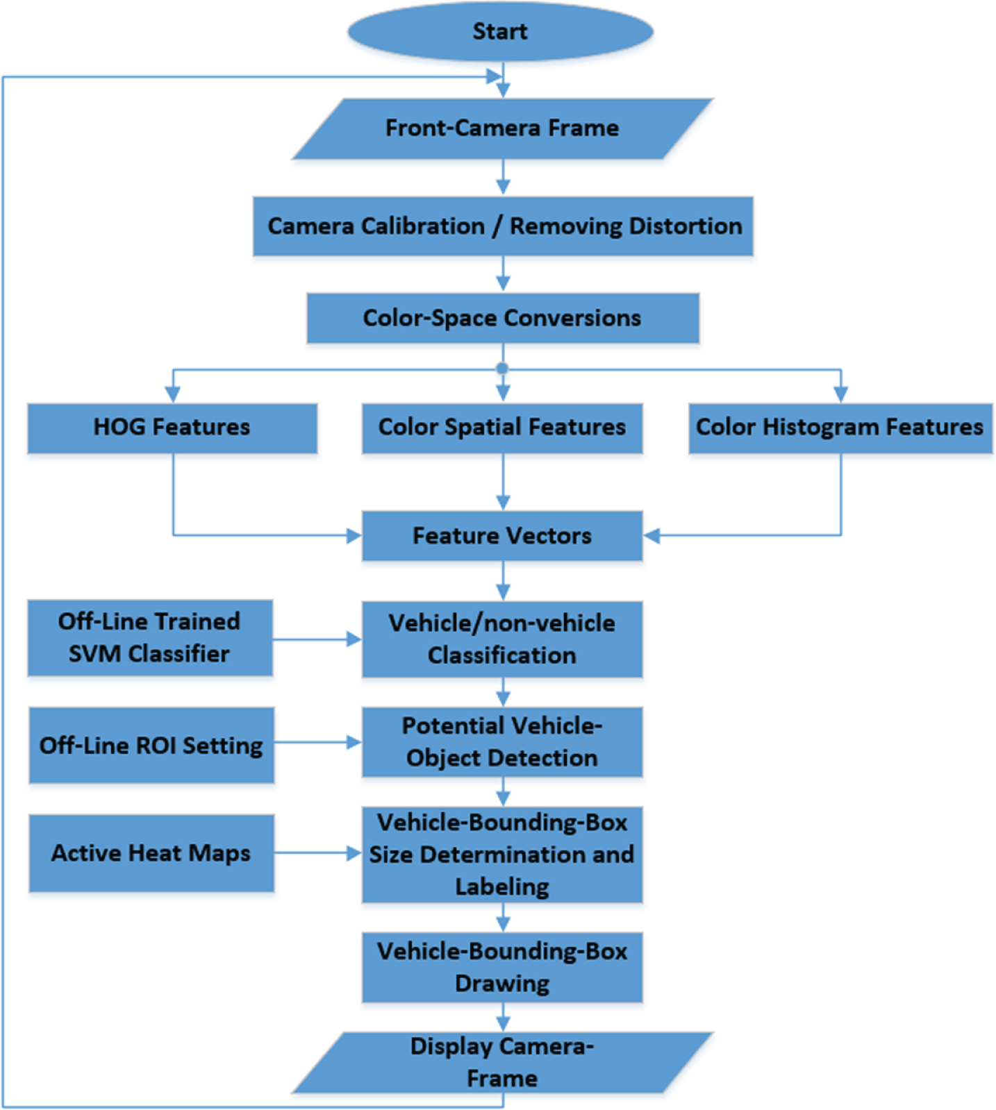
The RT_VDT Pipeline.
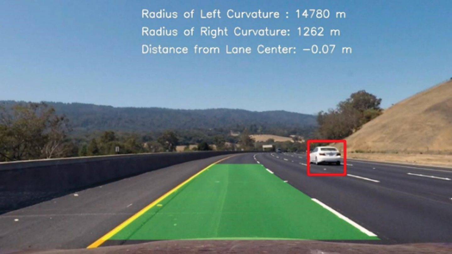
Detected Vehicle boundaries by the RT_VDT algorithm.
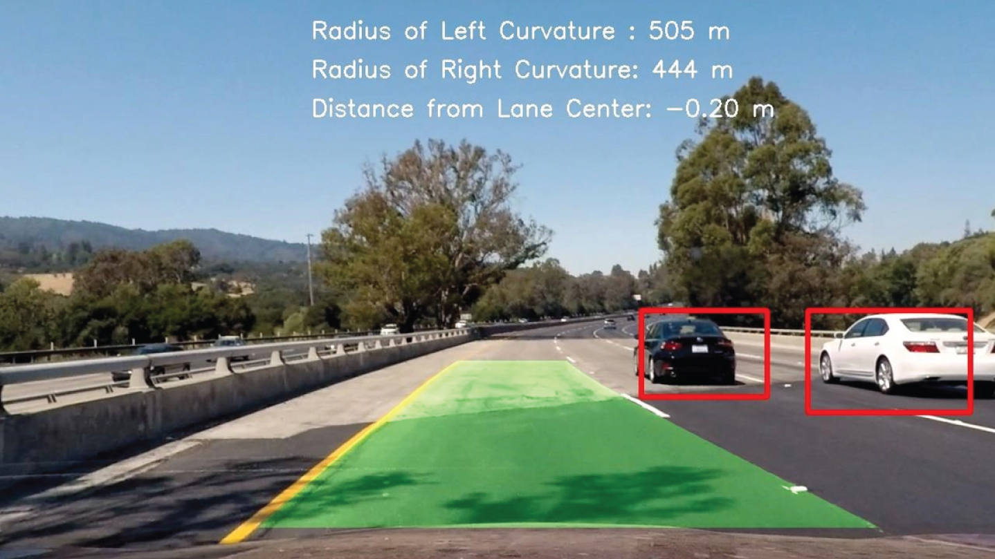
Detected Vehicles’ boundaries by the RT_VDT algorithm.
The HOG is a feature descriptor used in computer vision and image processing for the purpose of object detection [20].
For instance, to detect a specific object ‘O
bj
’ in a camera image the following steps can be followed: The camera image is converted to gray. Start by constructing a rectangle (or square) window that is 64 pixels tall by 64 pixels wide (the dimensions of the window are arbitrary depending on the designer choice). Use it to scan the grey camera image searching for O
bj
. The search is done by sliding the window both horizontally and vertically with a stride of 8 bits (as an example). The object O
bj
may have of course different sizes and occupy a bigger or small part of the image. Therefore, the analysis should be done not only on the original starting window (64×64) but also on a series (pyramid) of windows with an increment of 16 bits (as an example), like 80×80, 96×96, 112×112, etc. This pyramid of windows corresponds to larger portions of the original camera image where O
bj
or part of it could be inside one of them. In each step of the windows slide, the HOG features are computed and get associated with the center position of the corresponding window as a matter of “feature localization”.
To compute the HOG features, the input to the algorithm is expected to be a certain window ‘W I ’ from a gray-level image, possibly from a pyramid, and the workflow continues as follows and shown in Fig. 4:
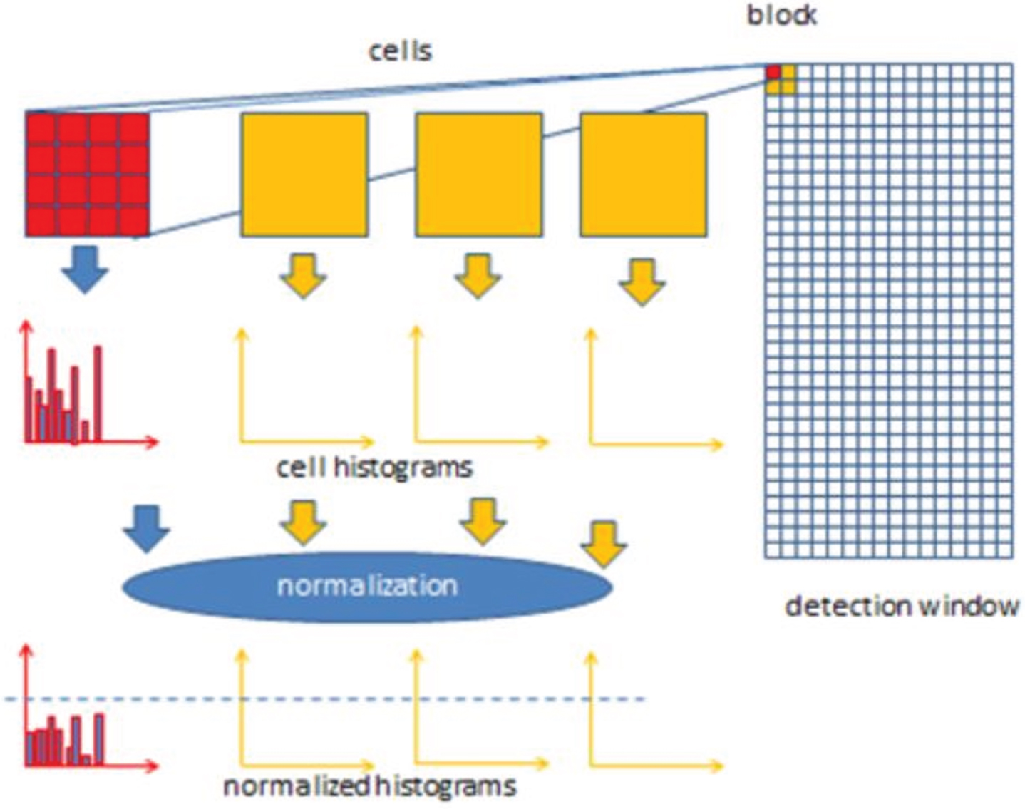
The Histogram of Oriented Gradients Workflow.
Calculate the two gradient components G
x
and G
y
of the gradient of W
I
by central differences:
The calculated gradient is then converted to polar coordinates as below, with the angle constrained to be between 0° and 180°. As a result, gradients that point in opposite directions are computed as:
Construct the cell orientation histograms by dividing the window W
I
into adjacent, non-overlapping cells of size C×C pixels (could be C = 8). In each cell, calculate the histogram of gradient orientations that are enclosed (binned) into B bins (could be B = 9). If the bins are numbered 0 through B-1 and have width
The block normalization step is then carried out by grouping the cells together into overlapping blocks of 2×2 cells each. Therefore, each block has a size of 2C×2C pixels. Accordingly, each two horizontally or vertically consecutive blocks overlap by two cells, that is, the block stride is C pixels. Consequently, each internal cell is covered by four blocks. The four-cell histograms in each block are concentrated into a single block feature b and then the block feature ‘b’ get normalized by its Euclidean norm as:
The normalized block features are then concatenated into a single HOG feature vector h, which is normalized as follows:
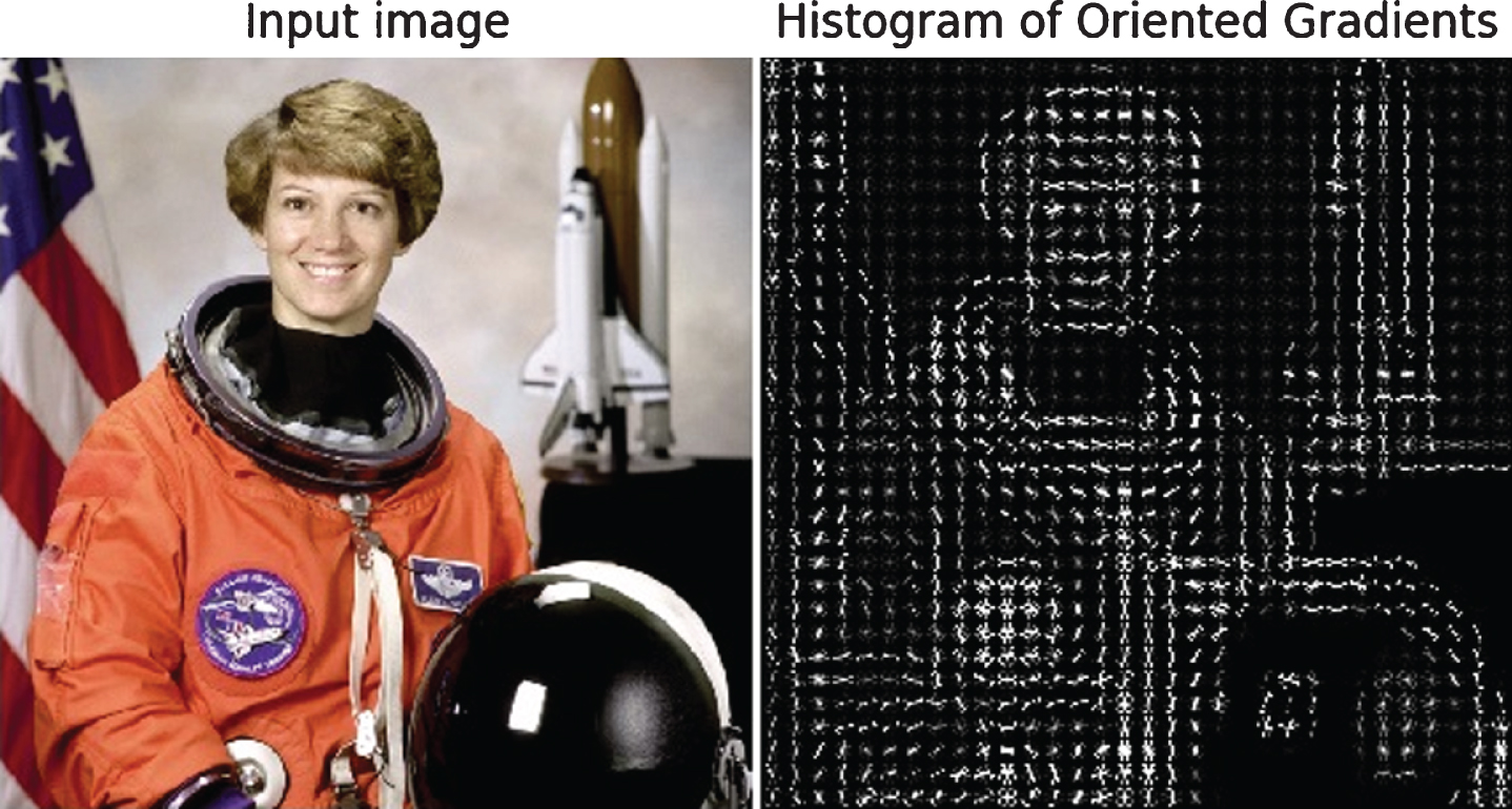
Results of applying HOG.
Support Vector Machine (SVM) [26] is a supervised learning model with an associated learning algorithm that analyzes data used for classification and regression analysis [27]. Given a set of training examples, each marked as belonging to one or the other of two categories, an SVM training algorithm builds a model that assigns new examples to one category or the other, making it a non-probabilistic binary linear classifier.
Given a training dataset of n points of the form
Any hyperplane can be written as the set of points
If the training data is linearly separable, the optimization problem can be written as follows:
The
If the training data is not linearly separable, the hinge loss function is introduced as
This function is zero if the constraint
where the parameter λ plays a role of determining the tradeoff between two opposing requirements: one is increasing the margin-size and the other is ensuring that the
If a nonlinear classification rule needs to be learned, and which this non-linear rule corresponds to a linear classification rule for the transformed data points
The coefficients
Finally, new points (
The conversion from three dimensional (3D) real-world scene to a two dimensional (2D) one, exhibits by a camera, results in image distortion, as the transformation from 3D→2D is not perfect. Actually, the shape and size of objects get distorted (changed) in the resulting 2D image from the original 3D appearance. Therefore, before using the resulting 2D camera images, this distortion needs to be undone so that the correct and useful information can be extracted and analyzed.
The construction of real cameras includes using a curved lens to form an image. The light rays usually bend around the edges of these lenses with low or high degrees depends on the focus and position of objects. Therefore, distortion at the images’ edges happens, in a way that lines or objects appear to be more or less curved than their actual reality. This effect is called the “radial distortion”, and represents the principal source of distortion.
Moreover, there is another main source of distortion that is the “tangential distortion”. This distortion happens when the camera’s lens is not perfectly aligned parallel to the image plane that is associated with the camera sensor. This produces a tilt effect to the image, which shows objects nearer or farther away than they actually are.
There are three needed coefficients to correct for radial distortion: k1, k2, and k3. To correct the appearance of radially distorted points in an image, one can use a correction formula.
In the following Equation (19), and Equation (20), (x, y) is a point in a distorted image. To undistort these points, the first step is to use OpenCV [29] to calculate r, which is the known distance between a point in an undistorted (corrected) image (x
corrected
,y
corrected
) and the center of the image distortion, which is often the center of that image (x
c
, y
c
). This center point (x
c
, y
c
) is sometimes referred to as the distortion center. These points are illustrated below in Fig. 6.
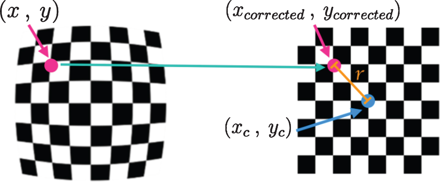
Points in a distorted and undistorted (corrected) images.
There are two more coefficients that account for tangential distortion: p1 and p2, and this distortion can be corrected using a different correction formula as given by Equation (21) and (22).
To correct for the mentioned distortions, images of known shapes (chessboard images) are used. Selected points in the distorted plans are then mapped to undistorted plans as shown in Fig. 7. Accordingly, the camera images will be calibrated. The following procedure is implemented to undistort the captured camera images and improve the image quality:
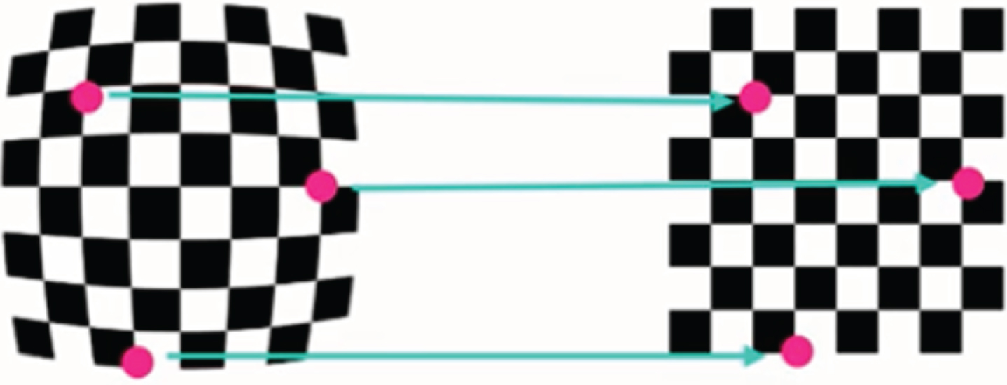
Mapping from a distorted chessboard image to an undistorted one.
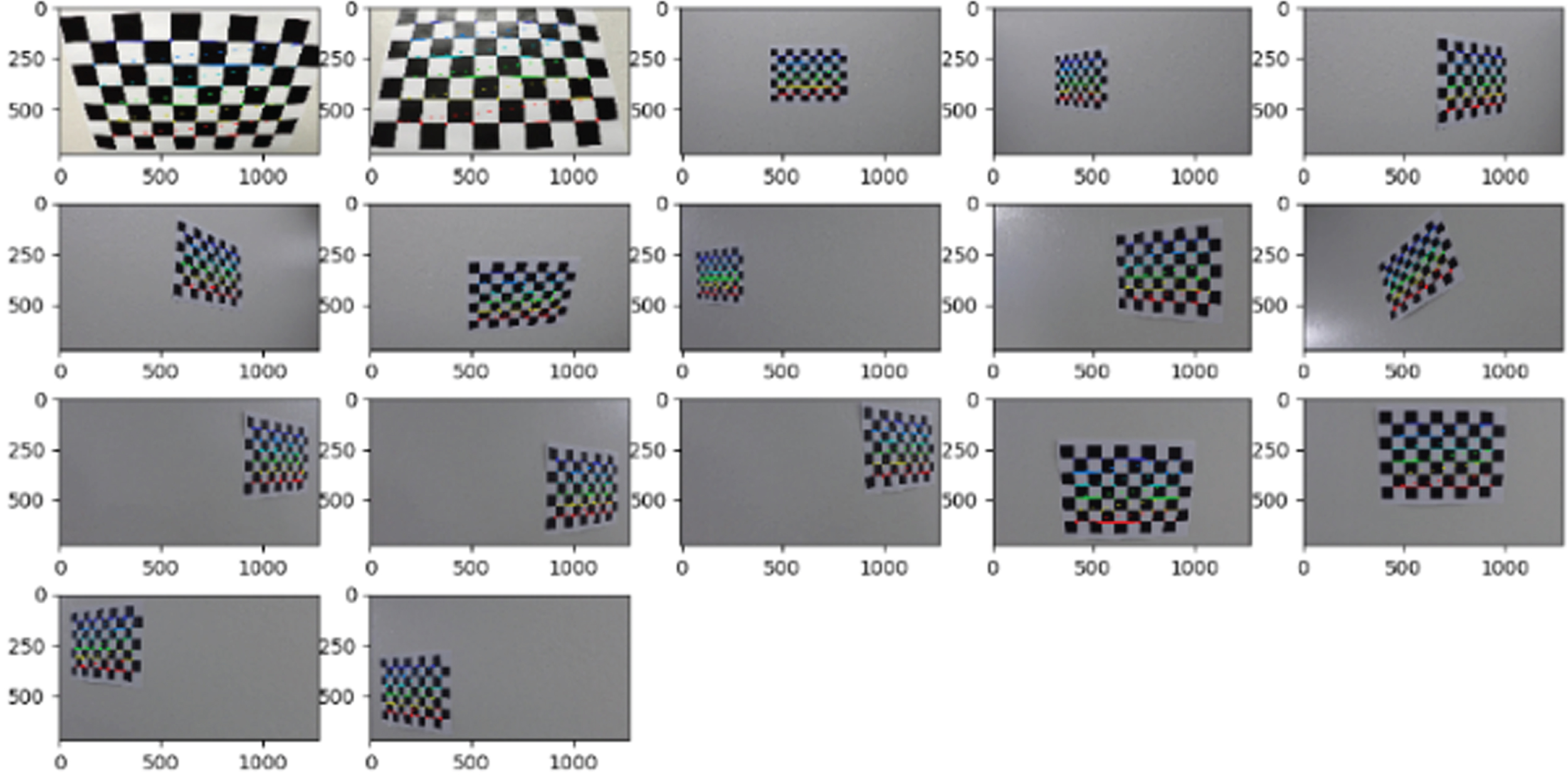
Chessboard images used for calibration with corners drawn.
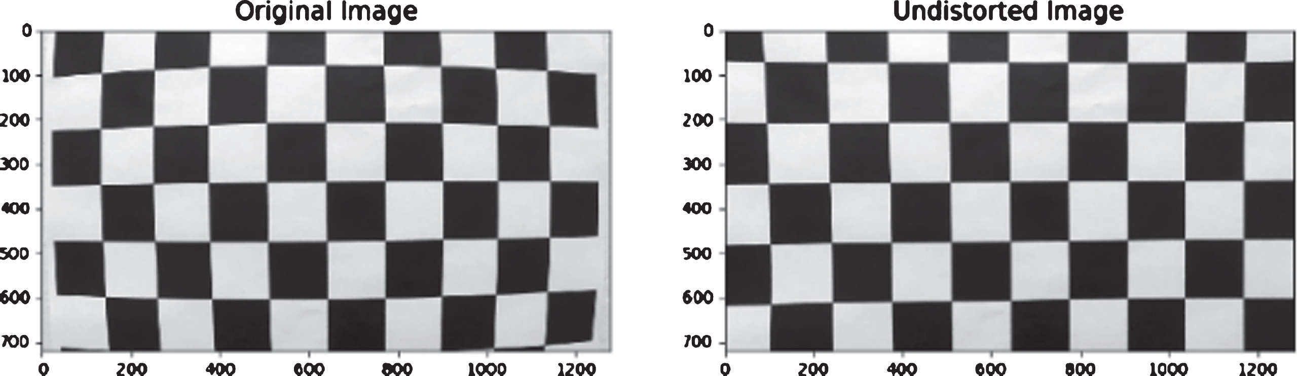
A test chessboard image with distortion removal.
Figure 10 provides an example of applying the camera calibration procedure on one of the test images.
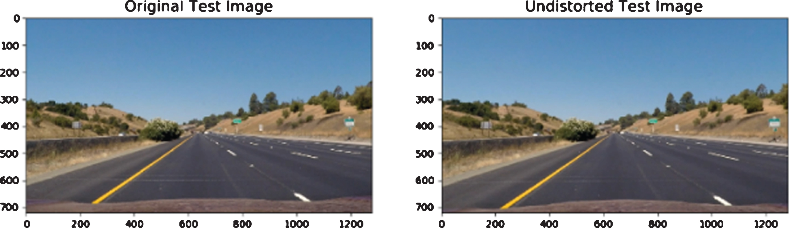
Camera calibration effect (undistortion of images).
In this section, the steps to build a classifier based on the SVM algorithm described in Section 4 will be explained in detail, and it is given the abbreviation “SVMC”.
Training data preparation
The data preparation steps to train the SVMC is summarized as follows
These collections with an unzipped size of 149MB. Data Augmentation: The data is augmented by flipping all the images around the “Y” axis. As a result, the training data become a total of 35,520 images.
Training data visualization
The following steps describe the implemented data visualization steps in order of execution:

Visualization of 50 randomly selected vehicle images.

Visualization of 50 randomly selected non-vehicle images.

Visualization of HOG features for vehicles and non-vehicle images.
The following steps describe the implemented images feature extraction functions in order of execution:
Using the color spatial features and ‘spatial size = (32, 32)’ results in a feature vector of 32×32×3 = 3072 elements. Using the color histogram features and ‘histogram bins = 32’ results in a feature vector of 32×3 = 96 elements. Using the HOG features and ‘gradient orientations cells = 9’, ‘pixels per cell = 8×8’, ‘cells per block = 2×2’, and using all color channels results in a feature vector of 7×7×2×2×9 = 1764 ×3 = 5292 elements. If all the above functions are used the resulting feature vector will be of the following length: 3072 + 96 + 5292 = 8460 elements.
Training the classifier
The following steps are used to build up and train the vehicle/non-vehicle SVMC classifier: Compiling a training data set “X” of 35,520×8,460 size which includes 35,520 vehicle/nonvehicle feature vectors of length 8,460 each. This training set represents the input to the classifier. The feature sets must be scaled; before combining them together; using the SciKit-Learn “StandardScaler().fit()” function [35]. Figure 14 shows the visualization of raw and normalized feature vectors for a vehicle image. Compiling an output training set “Y” of a 35,520×1 size in which each element is of a Boolean value of 1 = >vehicle or 0 = >non-vehicle. Shuffle the training sets randomly and split them to 80% for training and 20% for testing using the SciKit-Learn “train_test_split()” function. Using a Linear Space Vector Machine Classifier function “LinearSVC()” of the Sci-Kit Learn library [36], the model got trained with high accuracy (above 97.7%) in almost all the selected parameters combinations. Then the trained model is tested on the prepared test images. The results were not good in several cases. Extreme experimentations have been done with many parameter combinations, however, the results still were not acceptable. After several trials and errors, it is found that the color spatial features are taking a significant portion of the feature vector length (>36%) without adding a real value (sometimes even represents a confusing element) to the distinction between the vehicles / non-vehicles. Moreover, the color histogram features are of a very insignificant contribution (∼ 1.1%) of the feature vector as well as to the distinction between vehicles / non-vehicles. Therefore, both the color special and histogram features have been removed from the feature vector and keeping only the HOG features. By doing that, this results in a reduction in the length of the feature vector from 8,460 to 5,292 features only. This is off-course simplifies the training and the real-time application of the algorithm, and results in a huge reduction of processing and training time. The new Linear SVC classifier with a training data set of size = 35,520×5,292 is constructed using several color spaces with the training results shown in Table 1. Almost all the color spaces produced comparable results except the “RGB”. The “LAB” color space produces the fastest performance in both training and prediction with second to highest accuracy behind the “YUV”. However, while testing on test-images “YUV” produced false positives more than “LAB”. Therefore, “LAB” color space is selected for the next steps. The training time of the SVC does not affect the performance of the RT_VDT pipeline as it is done offline; however, the prediction time for the labels does affect the performance, as it will be part of the detection time for each camera frame.

Visualization of feature vectors for vehicles’ images.
Linear SVC training results
The following steps constitute the pipeline used in the detection and tracking of other vehicles on the road (RT_VDT). These steps are presented in order of execution:
“orient = 9” defining the number of histogram bins per cell and it is used for the HOG feature extraction for images or video frames. “pix_per_cell = 8” defining the number of HOG pixels/cell. In this case, the cell will be 8×8 pixels. “cell_per_block = 2” defining the number of HOG cells/block. In this case, the cell will be 2×2 cells. xstart, xstop, ystart, ystop: these 4 parameters define a rectangular area on the image or frame that represents the region of interest (ROI) in which the function searches for a vehicle by the sliding windows technique. “step_size = 2” defining how many cells to step (or to slide) to construct a new search window that will overlap with the previous search window. “Scale_Step = 0.25” defining the step at which the search window sizes increments from one search scan to the next. Scale_Multiplier_Start, Scale_Multiplier_End: two parameters defining the starting and stopping of the windows sizes increment while scanning the ROI area. The function uses the trained SVMC classifier model and applies it to each constructed search window. Sliding windows with different sizes are being constructed to cover the defined ROI as shown in Figure 15. This function as well may be applied several times with a different set of “a→g” parameters based on if it found necessary.

Sliding windows with different sizes scanning the ROI.
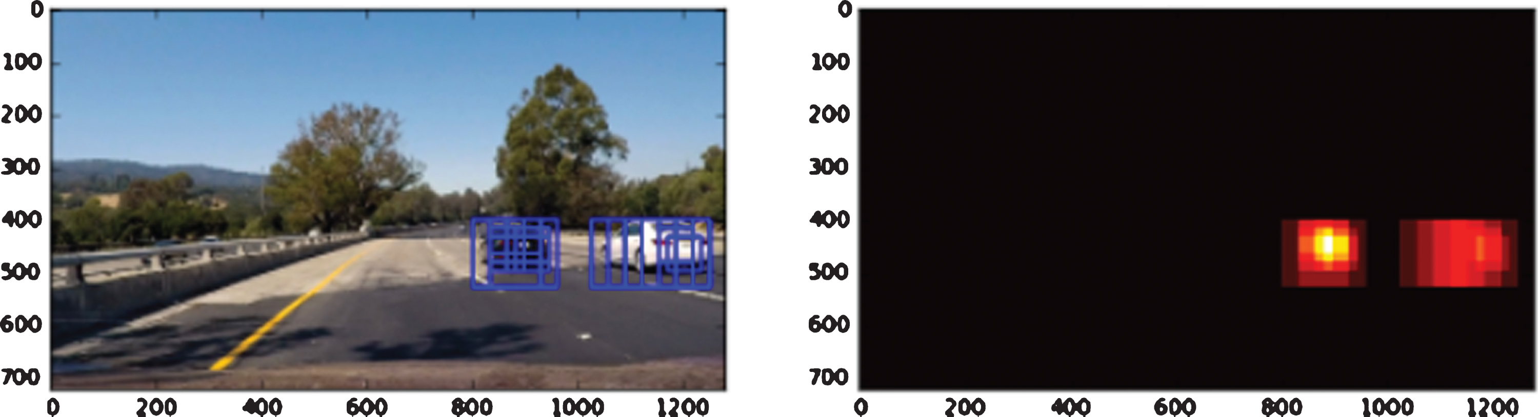
Detected vehicle boxes and the resulted heat-maps.
Figures 17 & 18 show examples of the results after the execution of the above pipeline on the test images that include shadow patterns that usually confuse vision-based algorithms.

The execution of vehicle detection and tracking pipeline.

The execution of vehicle detection and tracking pipeline.
The developed RT_VDT algorithm is further tested on various images representing different scenarios. The results show that the algorithm performs very well under different conditions (at full sunrise, at sunset, with shadows, without shadows, with cars on the other lanes and without). Furthermore, for robustness testing and validation of the developed pipeline, the algorithm is applied to several real-time video samples representing different driving conditions. The RT_VDT proved to be very robust in all the pre-mentioned conditions as shown in Figures 2 and 3. However, the scattered areas of shadows have an effect on the precision of producing the vehicles’ boundary boxes as shown in 17 and Fig. 18. However, the results are still acceptable and produce functional output.
As shown in Figure 2, Figure 3, Figure 17 and Figure 18 the images include as well lane detection results from the work in [6].
The pipeline proved to be acceptably fast in execution in real-time. Using an Intel Core i5-4200U @1.6GHz (2 cores) with 8GB RAM which very moderate computational platform, the following measurements are collected for two testing video streams:
The lowest measured processing speed is 10.01 frames per second, which is considered adequate as per the recommended performance for this application [17]. Therefore, the more powerful computational hardware if employed should significantly enhance the real-time performance of the proposed pipeline.
For the assessment of the RT_VDT performance, the experimental results are evaluated based on the three statistical measures test of a binary classification [37]: Precision, Recall and Intersection over Union (IoU). Precision measures how accurate the predictions are which is indicated by the proportion of actual-positive samples to all positively-identified samples. Recall measures the proportion of actual positive samples that are correctly identified (e.g., the percentage of vehicle images, which are identified as a true car image). IoU measures It measures the overlapping percentage between the predicted area and the ground-truth area, which is to measure how good our detector is with respect to the ground-truth. Their expressions are:
The well-established average precision (AP) and intersection over union (IoU) metrics [37] that has been widely used to assess various vehicle detection algorithms are used here to evaluate the performance and compare it to the state-of-the-art techniques [38]. Single-Shot Detector (SSD) [38] is one of the state-of-the-art single-stage detectors, which make predictions by utilizing different resolutions of feature maps. You Only Look Once (YOLO) [39] is another type of single-stage detector, which makes predictions by regarding raw image data as a 7×7 grid. Moreover, Faster R-CNN [40] is another state-of-the-art detector that was the first to incorporate Region Proposal Network (RPN) as a Region of Interest (RoI) candidate extractor.
Table 3 below compares the proposed RT_VDT technique to the state-of-the-art ones that are based on deeplearning (e.g. SSD, YOLO, and Fast R-CNN), and this comparison is based on the KITTI dataset [14]. It is obvious that the deeplearning algorithms have higher performance than the RT_VDT in terms of detection precision, however, at the expense of enormous computational cost. For example, YOLOv2 shows high performance in terms of Average Precision (AP) as well as real-time performance on a high-end GPU (∼37 FPS). However, on a very high-grade CPU, the performance is extremely poor (∼0.08 FPS) compared to the 12.52 FPS of the RT_VDT on a lower-cost affordable CPU. For ADAS applications with limited computational resources, the feature cost is as important as accuracy, and a delicate balance between them is what the automotive industry requires.
Computation Speed for the RT_VDT Algorithm
Comparison of different techniques on the KITTI car-detection validation set
The RT_VDT pipeline is executed as well on the google Colab cloud platform [42] in two different modes: GPU (NVIDIA Tesla K80, 13GB RAM) and TPU (v2) [42]. The best results achieved on the GPU is 0.058 Sec and on TPU is 0.073 sec. These trials indicating that not much difference in performance is taking place compared to the results on CPUs. The existence of the GPU added only an improvement of 27% in computational speed, while the TPU is adding only 7.5%. The justification for these results is that the GPU is mainly speeding the matrix operations and the developed pipeline does involve much of matrix operations. Moreover, the TPU is mainly designed to speed up computation based on tensors which are not used in the formulation of the RT_VDT algorithm [43]. The performance of the RT_VDT algorithm is also illustrated in Fig. 19 and Fig. 20 below.

Detected Vehicle boundaries by the RT_VDT algorithm on the KITTI dataset - 1.
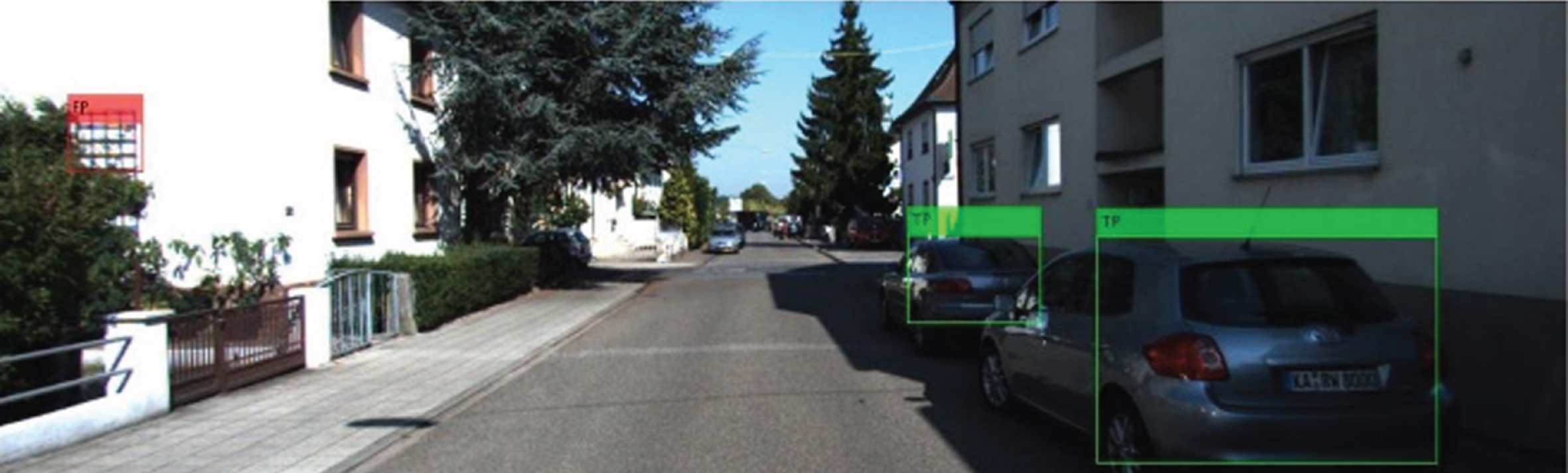
Detected Vehicle boundaries by the RT_VDT algorithm on the KITTI dataset - 2.
The following points shed some light on some technical tricks and aspects that have been tried or implemented in the described pipelines:
Conclusion
In this paper, reliable and sophisticated vehicle detection and tracking technique based on handcrafted-feature extraction is developed, presented thoroughly and given the name RT_VDT. RT_VDT uses a pipeline of distinguished color spaces such as LAB, YUV, LUV, etc. In addition, it uses computer-vision algorithms like HOG features, and machine learning algorithms like Support Vector Machines. Besides, the pipeline uses a comprehensive image distortion suppression and camera calibration techniques to produce undistorted road images suitable for more accurate vehicle detection. Furthermore, several sanity-check tricks are exercised to improve the robustness of the used techniques. The proposed RT_VDT technique needs only raw RGB images from a single CCD camera mounted behind the front windshield of the vehicle. The performance of the RT_VDT algorithm is tested and evaluated using many stationary images and several real-time videos. The validation results show a fairly accurate and robust detection with a slight insignificant deviation in one scenario where complex shadow patterns exist. The measured throughput (execution time) using an affordable CPU proved that the RT_VDT is very suitable for real-time vehicle detection even without adding further processing power like GPUs. Furthermore, the performance of RT_VDT technique is compared to the state-of-the-art deeplearning ones on the KITTI dataset. The deeplearning algorithms have higher performance than the RT_VDT, however, at the expense of much higher computational cost (high-end GPUs). However, on lower-cost CPUs, the RT_VDT real-time performance clearly shows that it is fitting for ADAS functions or self-driving cars. Future work will focus on augmenting the technique with the detection and tracking pedestrians and cyclists.
Footnotes
Acknowledgments
This work used the High-Performance Computing (HPC) facilities of the American University of the Middle East, Kuwait.