Single-machine scheduling problem with fuzzy time delays and mixed precedence constraints

Abstract

In this paper, we study the single-machine scheduling problem and obtain some new results on the special time-delay structure and mixed precedence constraints. We first demonstrate the complexity of the ordinary problem under different circumstances and obtain two cases, namely a polynomial solvable case and an NP-complete case. Then, we present a fuzzy extension of the ordinary problem, based on which a representation of the non-dominated solutions is given for the fuzzy scheduling problem. Finally, we demonstrate the complexity of fuzzy extension problems under different time delays by proposing corresponding algorithms.

Keywords

Single-machine scheduling problem mixed precedence constraints fuzzy time delays makespan complexity

1 Introduction

Single-machine scheduling problem with precedence constraints has been the subject of intensive research since the late 1960s [1 –10]. The ordinary precedence constraints are given by a strict binary partial relation on the set of jobs and reflect the ordering between jobs, which is not liable to any change under any circumstance. To describe a more flexible situation, Ishii and Tada first applied fuzzy precedence constraints to single-machine scheduling problem [11]. The fuzzy precedence constraints, which can be broken in some cases, reflect the satisfaction level with respect to the precedence between jobs. Machine scheduling problems with such constraints may occur in many situations in modern automated systems. Levner and Vlach [12] extended the problem model to a mixed precedence structure that includes both ordinary and fuzzy precedence constraints. They demonstrated that the two types of precedence constraints not only have different physical natures, but also require different algorithmic treatments in the scheduling problems. Xie et al. [13] investigated a bi-criteria single-machine scheduling problem involving fuzzy precedence constraints and fuzzy due dates. Through the search of non-dominated schedules, they constructed an O (n³) optimal algorithm. Li et al. [14] first applied fuzzy precedence constraints to a single-machine batch scheduling problem to minimize the makespan and maximize the minimum value of the desirability of the fuzzy precedence. They solved the problem by seeking non-dominated batch sequences. Shortly thereafter, Li et al. [15] applied fuzzy precedence constraints to a single-machine parallel-batching problem with a fuzzy due date, and presented an efficient algorithm to seek a non-dominated solution. Li et al. [16] considered a single machine due date assignment scheduling problem with precedence constraints and controllable processing times in fuzzy environment. They demonstrated the complexity of the scheduling problem and provided a polynomial time algorithm for the special case of the problem. More applications of fuzzy precedence constraints can be seen in the recent review [17].

Another stream of research considers single-machine scheduling problems with time-delay constraints. Wikum et al. [18] applied generalized precedence constraints to a single-machine scheduling problem to minimize the makespan, and demonstrated that the problem is computationally intractable. The generalized precedence constraints are actually time-delay constraints specifying that when job J_i precedes job J_j, the time between the completion of job J_i and the start of job J_j must be within a specified range. The range of time delays may depend on the machine and the jobs under consideration. Such time delays resemble setup times, but differ in an essential way; setup times can only occur between two consecutively scheduled jobs, whereas time delays can occur between any two jobs, even if other jobs are scheduled between them. Finta and Liu [19] investigated a single-machine scheduling problem with precedence delays for the minimization of the makespan. They showed that the problem is NP-hard when jobs have unit processing times and precedence delays have integer lengths, and provided an O (n²) optimal algorithm when jobs have arbitrary integer processing times and precedence delays have unit lengths. Muthusamy et al. [20] considered a fuzzy extension of one of the polynomial solvable cases of a single-machine scheduling problem with time delays studied by Wikum et al. [18]. The extension allowed time delays and precedence relations to be fuzzy. They evaluated feasible schedules by three measures of performance, and demonstrated that the problem of finding a set of non-dominated feasible schedules can be solved in polynomial time. Subsequently, Xie et al. [21 –23] investigated the single-machine scheduling problem involving the same fuzzy time-delay structure as that proposed by Muthusamy et al. [20]. Time-delay constraints have received considerable attention from researchers, and have been applied not only to various machine scheduling problems [24 –30], but also to robust control [31], economy model [32], neural networks [33, 34] and in-vehicle network [35].

As two important branches in the field of scheduling theory, the combination of precedence constraints and time delays has aroused the interest of some researchers [20 , 35]. Muthusamy et al. [20] and Xie et al. [22] applied time delays and precedence relations to single-machine scheduling problem. Darbandi et al. [35] investigated the holistic schedule which satisfy delay constraints and precedence constraints between tasks schedules and messages transmissions on in-vehicle networks. The fuzzy environment describes a more flexible situation and has better universality. In this paper, the single-machine scheduling problem with special time-delay structure and mixed precedence constraints including both ordinary and fuzzy precedence constraints is investigated. Our time-delay structure, in which there exists a job that has always been in the first position in any feasible schedule, is different from those discussed in the existing literature [18 , 20–23]. To the best of our knowledge, such a problem has not been studied. We will demonstrate the complexity of the ordinary problem under different circumstances and present fuzzy extension of the ordinary problem. Time delays and precedence constraints are to be fuzzy in the fuzzy extension. We evaluate feasible schedules of the fuzzy extension by three measures of performance: the makespan, the degree of satisfaction with fuzzy time delays, and the degree of satisfaction with mixed precedence constraints. Furthermore, we will demonstrate the complexity of fuzzy extension under different time delays by proposing corresponding algorithms. The universality of Lawler’s theorem is also proved when seeking non-dominant feasible schedules for the fuzzy extension.

The remainder of this paper is organized as follows. Section 2 presents the notation and ordinary problem description. In Section 3, we demonstrate the complexity of the ordinary problem, and in Section 4, we present the fuzzy extension of the ordinary problem. In Section 5, the complexity of fuzzy extension under different time delays is demonstrated by proposing corresponding algorithms. Section 6 presents two numerical examples, which is followed by the conclusion in Section 7.

2 Preliminary

There are n + 1 jobs, J₀, J₁, J₂, ⋯ , J_n, to be scheduled on a single machine. The objective is to minimize the makespan. It is assumed that the machine is continuously available and can process only one job at a time. Job splitting and pre-emption are not allowed. All jobs are available for processing at time zero. For simplicity, let p_i denote the processing time of job J_i for each i = 0, 1, 2, ⋯ , n, the beginning time of J_i is s (J_i), π is a feasible schedule, and C_i (π) is the completion time of job J_i in schedule π. Π is the set of all feasible schedules.

For the special time-delay structure, let J denote the set of jobs J₁, J₂, ⋯ , J_n, i.e., J = {J₁, J₂, ⋯ , J_n}. Every feasible schedule satisfies the time-delay constraints [l_i, u_i] for each J_i ∈ J, which means that the lower and upper bounds for time delay between J₀ and J_i are given by l_i and u_i, respectively, satisfying 0⩽ l_i ⩽ u_i < + ∞. In other words, job J₀ is always the first job in any feasible sequence, and the time between the completion of job J₀ and the start of job J_i ∈ J is at least l_i and no more than u_i (see Fig. 1). Note that the time delay between J₀ and J_i is actually an ordinary precedence constraint when l_i = 0 and u_i =∞.

Fig.1

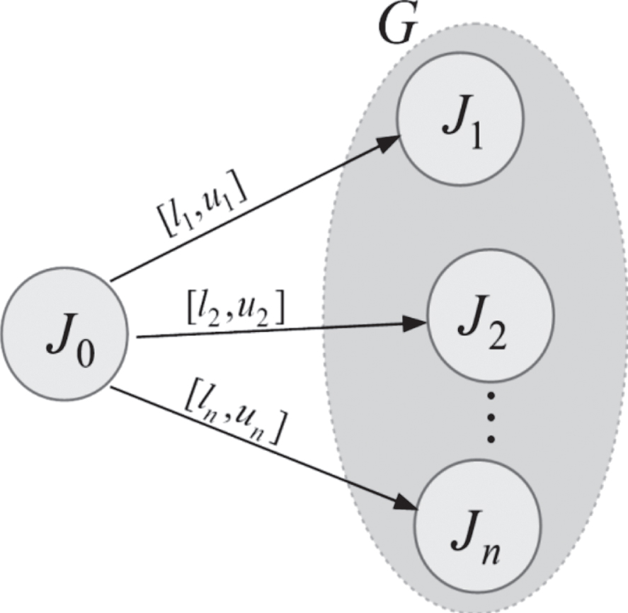
Time-delay constraints graph.

In addition, the jobs from the set J should be processed according to ordinary precedence constraints. For convenience of description, the precedence relations in the set J are represented by a directed graph G = G (V, A), where V is the set of jobs J_i for J_i ∈ J, and A is the set of arcs (J_i, J_j) such that J_i ≺ J_j, i.e., J_i precedes J_j. Jobs J_i and J_j are independent, which means that (J_i, J_j) and (J_j, J_i) are not in G = G (V, A).

As mentioned above, the ordinary problem can be formulated as follows.

Problem P: The single-machine scheduling problem with the objective to minimize the makespan is subject to time-delay constraints and ordinary precedence constraints.

3 Complexity of Problem P

In this section, we will demonstrate the complexity of Problem P with time delays in the following three cases:

[0, u_i] for i = 1, 2, ⋯ , n;

[l_i, ∞) for i = 1, 2, ⋯ , n;

[l_i, 1ptu_i], l_i > 0, and u_i is a nonnegative real number for i = 1, 2, ⋯ , n.

First, we give the following necessary lemmas.

Lemma 1. (Lawler and Moore [36]) Each job can be completed on time, consistent with the given precedence constraints, if and only if each job is completed on time in the sequence obtained by ordering jobs according to increasing values of ${\bar{d}}_{j}$ . ${\bar{d}}_{j} = min {d_{j}, min {d_{k} | J_{k} \in B_{j}}},$ where B_j = {J_i|J_j ≺ J_i, J_i ∈ J}.

Lemma 2. (Garey and Johnson [37]) Sequencing within intervals is NP-complete in the strong sense.

In the following, we present some new results for Problem P.

Theorem 1. In the case [0, u_i], Problem P can be solved in polynomial time.

Proof. The objective is to minimize the makespan and for the jobs to satisfy all time-delay constraints and ordinary precedence constraints. We only need to consider the semi-active schedule, in which there is no idle time during job processing, i.e., each job is scheduled as early as possible.

The time delays between J₀ and J_i ∈ J are given by [0, u_i], i = 1, 2, ⋯ , n. If we assume that job J_i ∈ J has due date d_i = p₀ + u_i + p_i, then there is a schedule that satisfies all due dates if and only if the schedule satisfies the time delays.

(“If”) For any feasible schedule π, assume that the completion time of job J_i ∈ J is C_i (π). Obviously, C_i (π) ⩽ p₀ + u_i + p_i = d_i for i = 1, 2, ⋯ , n. Hence, if we have a feasible schedule that satisfies the time delays, then it must satisfy all due dates.

(“Only If”) Suppose there is a schedule π that satisfies all due dates, that is, $C_{i} (π) ⩽ d_{i} = p_{0} + u_{i} + p_{i}, for i = 1, 2, \dots, n .$

It implies $C_{i} (π) - p_{i} - p_{0} ⩽ u_{i}, for i = 1, 2, \dots, n .$

Therefore, schedule π satisfies the time delays.

Thus, Problem P can be transformed to that of finding a schedule, if it exists, subject to the given precedence constraints, such that each job will be completed by its due date. According to Lemma 1, Problem P can be solved in O (n²) time. □

Lemma 3. In the case [l_i, ∞), if job J_i has release date r_i = p₀ + l_i for all i = 1, 2, ⋯ , n, then there is a schedule that satisfies all release dates if and only if the schedule satisfies the time delays.

Proof. The ordinary time delays between J₀ and J_i ∈ J are given by [l_i, ∞), i = 1, 2, ⋯ , n. For any feasible schedule π = (J₀, σ), σ = (σ (1) , σ (2) , ⋯ , σ (n)) is a permutation of jobs in J, where σ (k) represents the job that occupies position k in sequence σ, and s (σ (i)) denotes the beginning time of job σ (i). $\begin{matrix} s (σ (1)) & = & p_{0} + l_{σ (1)} \\ s (σ (t)) & = & max {s (σ (t - 1)) + p_{σ (t - 1)}, p_{0} + l_{σ (t)}}, \\ t = 2, \dots, n . \end{matrix}$ (1)

Obviously, in schedule π = (J₀, σ), the start time of job J_i must be at least r_i = p₀ + l_i for all i = 1, 2, ⋯ , n. Therefore, if we have a feasible schedule that satisfies the time delays, then it must satisfy these release times.

Suppose there is a schedule π = (J₀, σ) that satisfies all release times, that is, s (σ (i)) ⩾ r_σ(i) for each i = 1, 2, ⋯ , n. Then, for i = 1, 2, ⋯ , n, $\begin{matrix} 0 & ⩾ r_{σ (i)} - s (σ (i)) = p_{0} + l_{σ (i)} - s (σ (i)) \\ = C_{0} + l_{σ (i)} - s (σ (i)) . \end{matrix}$

This implies s (σ (i)) - C₀ ⩾ l_σ(i) for i = 1, 2, ⋯ , n. Therefore, schedule π = (J₀, σ) satisfies the time delays. □

Theorem 2. In the case [l_i, ∞), Problem P can be solved in polynomial time.

Proof. The ordinary time delays between J₀ and J_i ∈ J are given by [l_i, ∞), i = 1, 2, ⋯ , n. If we assume that each job J_i has release date r_i = p₀ + l_i for all i = 1, 2, ⋯ , n, according to Lemma 3, then Problem P can be transformed to the scheduling problem which minimizes the makespan subject to given release dates (no time delays) and ordinary precedence constraints.

In the following, we further demonstrate that the problem can be transformed into the scheduling problem that minimizes the makespan only subject to the revised release dates. Similar to the above theorem, we only need to consider the semi-active schedule.

Revise the release dates, make $r_{i}^{'} + p_{i} ⩽ r_{k}^{'}$ for J_i ≺ J_k. Assume, without loss of generality, that the jobs are numbered in such a way that J_i ≺ J_j implies i ⩽ j. For all i = 1, 2, ⋯ , n, let $\begin{matrix} B_{i} & = {J_{k} | J_{k} ≺ J_{i}, J_{k} \in J}, \\ r_{i}^{'} = max {r_{i}, max {r_{k}^{'} + p_{k}} | J_{k} \in B_{i}} + i ɛ, \end{matrix}$ where ɛ is a small number, and iɛ is used to break ties. It is important to note that J_i ≺ J_j implies $r_{i}^{'} ⩽ r_{j}^{'}$ . This implies that we construct a new job set with release date $r_{i}^{'}$ for each job J_i ∈ J, and one can ignore the precedence constraints.

The makespan can be minimized, subject to the given precedence constraints, if and only if the new jobs are ordered according to increasing values of $r_{i}^{'}$ .

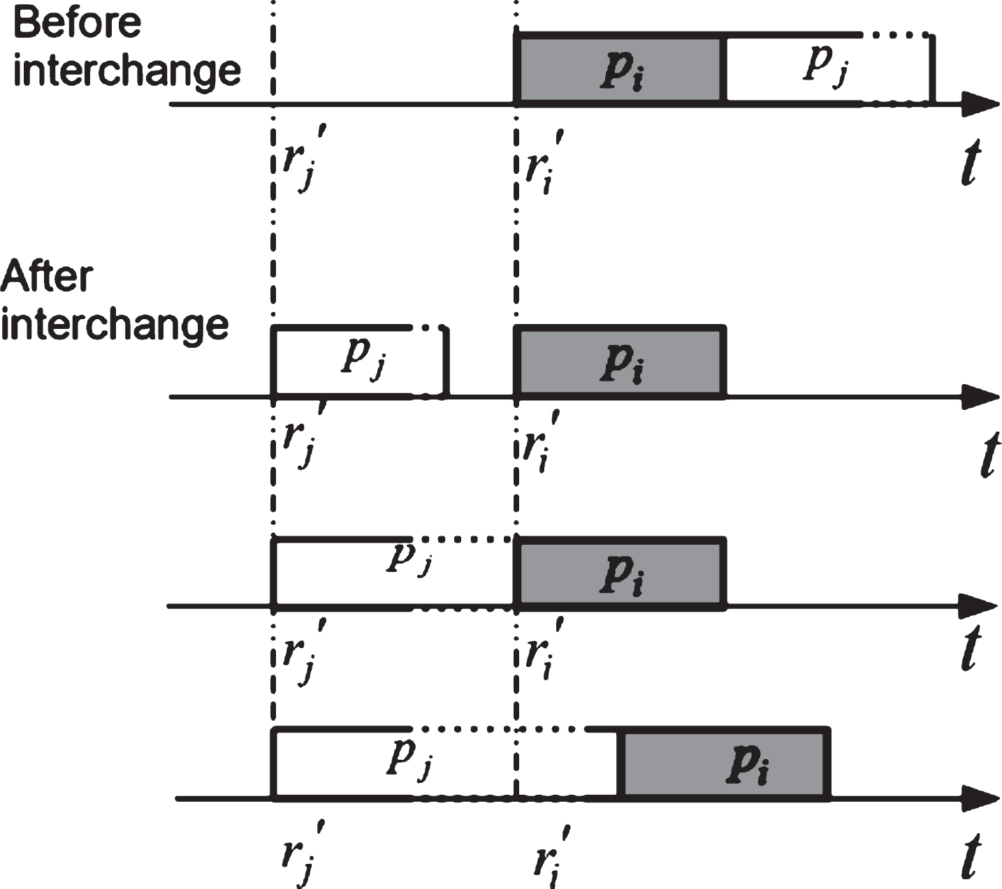
The “if” part is obvious, so we consider that there exists a hypothetical sequence that minimizes the makespan, but in which the jobs are not ordered according to increasing values of $r_{i}^{'}$ . Let J_i,J_j be a consecutive pair of jobs in this hypothetical sequence, with $r_{i}^{'} > r_{j}^{'}$ . It cannot be the case that J_i ≺ J_j, because that would imply $r_{i}^{'} ⩽ r_{j}^{'}$ , contrary to assumption. Hence, if we interchange the positions of J_i and J_j, we do not violate the precedence constraints. Further analysis reveals that if this hypothetical sequence can minimize the makespan, by interchanging the positions of J_i and J_j (see Fig. 2), we can get $max {r_{i}^{'}, r_{j}^{'} + p_{j}} + p_{i} ⩽ r_{i}^{'} + p_{i} + p_{j}$ , which results in a smaller makespan. This is contradictory to the hypothesis.

Fig.2

Interchange the positions of J_i and J_j.

Therefore, Problem P under consideration can be transformed to the scheduling problem that minimizes the makespan, and is only subject to the revised release dates. We can obtain the optimal schedule by sequencing the new jobs according to increasing values of $r_{i}^{'}$ .

The modification of release dates requires O (n²). After this, the jobs are ordered according to increasing $r_{i}^{'}$ in O (n log n) time. Hence, Problem P can be solved in O (n²) time. □

Theorem 3. In the case [l_i, 1ptu_i], Problem P is NP-complete in the strong sense.

Proof. According to Theorem 1 we can know that Problem P in the case [0, u_i] is equivalent to the revised due dates problem, and we determine that Problem P in the case [l_i, ∞) is equivalent to the revised release dates problem from Theorem 2. Thus, for [l_i, 1ptu_i], Problem P is equivalent to the problem with both due dates and release dates, and the complexity result is given by Lemma 2. Problem P is NP-complete in the strong sense. □

Theorem 1 and Theorem 2 show that Problem P can be solved in polynomial time in the cases [0, u_i] and [l_i, ∞), respectively. Theorem 3 shows that Problem P is NP-complete in the strong sense in the case [l_i, 1ptu_i].

4 Fuzzy extension of Problem P

In what follows, we will consider fuzzy extension of Problem P while allowing time delays and precedence relations to be fuzzy.

In the case [0, u_i], time-delay constraints are fuzzified. We assume that U_i is a fuzzy upper bound of the time delay between J₀ and J_i. U_i can be formulated as the fuzzy interval $[{\underline{u}}_{i}, {\bar{u}}_{i}]$ , where ${\underline{u}}_{i}$ and ${\bar{u}}_{i}$ are nonnegative real numbers and ${\underline{u}}_{i} < {\bar{u}}_{i}$ . The degree of satisfaction of customers with respect to time delay x_i between J₀ and J_i is f_i (x_i). $f_{i} (x_{i}) = {\begin{matrix} 1 & if x_{i} ⩽ {\underline{u}}_{i} \\ \frac{{\bar{u}}_{i} - x_{i}}{{\bar{u}}_{i} - {\underline{u}}_{i}} & if {\underline{u}}_{i} < x_{i} < {\bar{u}}_{i} \\ 0 & if x_{i} ⩾ {\bar{u}}_{i} . \end{matrix}$ (2)

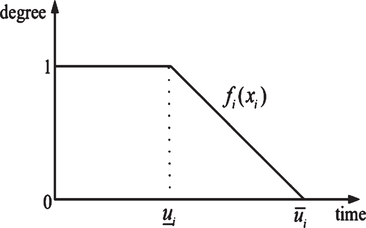
The crisp time delay u_i can be interpreted as the limit case for ${\underline{u}}_{i} = {\bar{u}}_{i} = u_{i}$ . If time delay x_i between J₀ and J_i is less than time ${\underline{u}}_{i}$ , there is a maximum degree of satisfaction, which is 1. As the time delay x_i increases, the degree of satisfaction will decrease from 1 to 0. Time delay x_i is infeasible whenever $x_{i} ⩾ {\bar{u}}_{i}$ (see Fig. 3).

Fig.3

Degree of satisfaction with fuzzy upper bound.

In the case [l_i, ∞), the upper bound of the time delay is infinite. We assume that the lower bound L_i of the time delay between J₀ and J_i is fuzzified. L_i can be formulated as the fuzzy interval $[{\underline{l}}_{i}, {\bar{l}}_{i}]$ , where ${\underline{l}}_{i}$ and ${\bar{l}}_{i}$ are nonnegative real numbers and ${\underline{l}}_{i} < {\bar{l}}_{i}$ . The degree of satisfaction of customers with time delay x_i between J₀ and J_i is f_i (x_i).

$f_{i} (x_{i}) = {\begin{matrix} 1 if x_{i} ⩾ {\bar{l}}_{i} \\ \frac{x_{i} - {\underline{l}}_{i}}{{\bar{l}}_{i} - {\underline{l}}_{i}} if {\underline{l}}_{i} < x_{i} < {\bar{l}}_{i} \\ 0 if x_{i} ⩽ {\underline{l}}_{i} . \end{matrix}$ (3)

The crisp time delay l_i can be interpreted as the limit case for ${\underline{l}}_{i} = {\bar{l}}_{i} = l_{i}$ . Time delay x_i between J₀ and J_i is considered as feasible whenever $x_{i} > {\underline{l}}_{i}$ , otherwise x_i is infeasible. As the time delay x_i increases, the degree of satisfaction increases from 0 to 1. If time delay x_i is more than time ${\bar{l}}_{i}$ , there is a maximum degree of satisfaction, which is 1 (see Fig. 4).

Fig.4

Degree of satisfaction with fuzzy lower bound.

In the case [l_i, 1ptu_i], we assume that the lower bound L_i and the upper bound U_i of the time delay x_i between J₀ and J_i are fuzzified. L_iand U_i can be formulated as the fuzzy interval $[{\underline{l}}_{i}, {\bar{l}}_{i}]$ and $[{\underline{u}}_{i}, {\bar{u}}_{i}]$ , respectively, where ${\underline{l}}_{i}$ , ${\bar{l}}_{i}$ , ${\underline{u}}_{i}$ and ${\bar{u}}_{i}$ are nonnegative real numbers and ${\underline{l}}_{i} < {\bar{l}}_{i} < {\underline{u}}_{i} < {\bar{u}}_{i}$ . The degree of satisfaction of customers with time delay x_i between J₀ and J_i is f_i (x_i).

$f_{i} (x_{i}) = {\begin{matrix} \frac{{\bar{u}}_{i} - x_{i}}{{\bar{u}}_{i} - {\underline{u}}_{i}} if {\underline{u}}_{i} < x_{i} < {\bar{u}}_{i} \\ 1 if {\bar{l}}_{i} ⩽ x_{i} ⩽ {\underline{u}}_{i} \\ \frac{x_{i} - {\underline{l}}_{i}}{{\bar{l}}_{i} - {\underline{l}}_{i}} if {\underline{l}}_{i} < x_{i} < {\bar{l}}_{i} \\ 0 if x_{i} ⩽ {\underline{l}}_{i} or x_{i} ⩾ {\bar{u}}_{i} \end{matrix}$ (4)

Time delay x_i between J₀ and J_i is considered as feasible whenever ${\underline{l}}_{i} < x_{i} < {\bar{u}}_{i}$ , otherwise x_i is infeasible. As the time delay x_i increases, the degree of satisfaction first increases from 0 to 1, and then decreases from 1 to 0. If time delay $x_{i} \in [{\bar{l}}_{i}, {\underline{u}}_{i}]$ , there is a maximum degree of satisfaction, which is 1 (see Fig. 5).

In addition, the jobs from the set J = {J₁, J₂, ⋯ , J_n} are subject to mixed precedence constraints, i.e., the jobs from J may be processed in ordinary precedence order or in fuzzy precedence order. Fuzzy precedence constraint is denoted by the membership function μ_ij for any two jobs J_i and J_j, which expresses the degree of satisfaction that job J_i is processed before job J_j. Because either J_i is processed before J_j or vice versa, we assume that μ_ji = 1 if 0 ⩽ μ_ij < 1. This can be interpreted as a normalization condition, and that μ_ji is the preferred order and has a satisfaction degree 1. Both μ_ij and μ_ji equal 1 if jobs J_i and J_j are independent.

Fig.5

Degree of satisfaction with fuzzy lower bound and fuzzy upper bound.

As mentioned above, the fuzzy scheduling problem can be expressed as follows.

Fuzzy Problem FP: The single-machine scheduling problem is subject to fuzzy time delays and mixed precedence constraints. The objectives of the problem are: 1) the makespan is to be minimized; 2) the minimum degree of satisfaction of fuzzy time delays is to be maximized; 3) the minimum degree of satisfaction of mixed precedence constraints is to be maximized.

The makespan of schedule π, denoted by $C_{max}^{π}$ , is defined as the maximum of the completion times of all jobs in π, i.e., $\begin{matrix} C_{max}^{π} = max {C_{i} (π) | i = 1, 2, \dots, n} \\ = max {p_{0} + x_{i} + p_{i} | i = 1, 2, \dots, n}, \end{matrix}$ (5) where x_i is the time delay between J₀ and J_i for i = 1, 2, ⋯ , n.

For every feasible schedule π, we denote the minimum degree of satisfaction of fuzzy time delays by $f_{min}^{π} = min {f_{i} (x_{i}) | J_{i} \in J} .$ (6)

For convenience, we denote the feasible schedule π = (J₀, σ), and σ = (σ (1) , σ (2) , ⋯ , σ (n)) is a permutation sequence of the jobs in J, where σ (k) represents the job that occupies position k in sequence σ. Then, for schedule π, the minimum degree of satisfaction with mixed precedence constraints is $μ_{min}^{π} = min {μ_{σ (i) σ (j)} | i, j = 1, 2, \dots, n, i < j} .$ (7)

The objective is to find an optimal schedule π to minimize the makespan, maximize the minimum degree of satisfaction with fuzzy time delays, and maximize the minimum degree of satisfaction with mixed precedence constraints. However, it is possible that no feasible schedule optimizes $C_{max}^{π}$ , $f_{min}^{π}$ , and $μ_{min}^{π}$ simultaneously. For multi-criteria scheduling problems, T’Kindt et al. proposed a variety of methods for the representation of solutions [39]. In this paper, we use non-dominated solutions to denote optimal solutions of the fuzzy problem. The vector $v^{π} = (C_{max}^{π}, f_{min}^{π}, μ_{min}^{π})$ consists of three elements. We say that vector v^{π
₁} dominates vector v^{π
₂} if $C_{max}^{π_{1}} ⩽ C_{max}^{π_{2}}$ , $f_{min}^{π_{1}} ⩾ f_{min}^{π_{2}}$ , $μ_{min}^{π_{1}} ⩾ μ_{min}^{π_{2}}$ , and at least one of these inequalities is strict. In this case, we also say that schedule π₁ dominates schedule π₂. A feasible schedule π is called non-dominated if and only if there exists no feasible schedule that dominates π. If $C_{max}^{π_{1}} = C_{max}^{π_{2}}$ , $f_{min}^{π_{1}} = f_{min}^{π_{2}}$ , and $μ_{min}^{π_{1}} = μ_{min}^{π_{2}}$ , we say that π₁ and π₂ are equivalent. Consequently, every equivalence class of schedules consists of all schedules with identical values of C_max, f_min and μ_min, and the set of all feasible schedules that are equivalent to a feasible schedule π is called the equivalence class of π.

5 Complexity of Problem FP

The fuzzy extension of the ordinary problem is more complicated and the ordinary problem is just a special case of the fuzzy problem. In the case of [l_i, u_i], Problem P is proved to be NP-complete in the strong sense, so its fuzzy extension FP must also be a strongly NP-complete problem. However the complexity of the corresponding fuzzy problem remains unknown when the ordinary problem is polynomial solvable. In this section, we will demonstrate that Problem FP is polynomial solvable by proposing corresponding algorithms in the case of [0, u_i] and [l_i, ∞) respectively.

Sort 0 < μ_ij < 1 in non-increasing order. Let the result be μ⁰ = 1 > μ¹ > μ² > ⋯ > μ^k > 0, where k is the number of different μ_ij. G⁰ (V, A⁰) is the mixed precedence digraph obtained from the ordinary precedence graph G (V, A) by adding to it all arcs (J_i, J_j) corresponding to the fuzzy precedence constraints with μ_ij = 1, i.e., $A^{0} = {(J_{i}, J_{j}) | μ_{ij} = μ^{0} and μ_{ji} \neq μ^{0}} .$

In this paper, we suppose the directed graph G⁰ (V, A⁰) is acyclic. G^l (V, A^l) is the mixed precedence digraph obtained from G⁰ (V, A⁰) by deleting all arcs (J_i, J_j) such that μ_ij = 1 and μ_ji ⩾ μ^l, i.e., $\begin{matrix} A^{l} = & {(J_{i}, J_{j}) | μ_{ij} = μ^{0} and μ_{ji} < μ^{l}}, \\ l = 1, 2, \dots, k . \end{matrix}$

5.1 In the case [0, u_i]

There are mixed precedence constraints between jobs from set J. The feasibility of schedules is further constrained by requiring that the time between the completion of J₀ and the beginning of J_i(J_i ∈ J) must be less than or equal to a given fuzzy number U_i.

5.1.1 Single machine f_min maximization problem

To solve the fuzzy problem FP, in this subsection, we consider a single-objective scheduling problem in which, instead of the mixed precedence relation, there is only ordinary precedence relation, and a single objective function f_min is to be maximized. The problem can be stated as follows.

Problem FP1: The single-machine scheduling problem, in which the minimum degree of satisfaction of fuzzy time delays is to be maximized, is subject to fuzzy time-delay constraints and ordinary precedence constraints.

Although there are fuzzy time delays between J₀ and jobs from J, the problem FP1 is similar to the well-known 1973 Lawler’s problem [38]. The difference between these two problems is that they have opposite objective functions. The problem discussed in this paper is to maximize the minimum of fuzzy monotone non-increasing functions, while Lawler’s problem is to minimize the maximum of the monotone non-decreasing functions. In the following result, we will prove that Lawler’s theorem remains feasible and valid for the proposed fuzzy monotone non-increasing functions in this paper.

Theorem 4. Let U denote the set of jobs that are not required to precede any others. Let p denote the sum of the processing times of all jobs, i.e., p = p₀ + p₁ + ⋯ + p_n. Let J_k be a job in U such that $f_{k} (x_{k}) = max_{J_{i} \in U} f_{i} (x_{i}) = max_{J_{i} \in U} f_{i} (p - p_{0} - p_{i}),$ (8) where x_i = p - p₀ - p_i. Then there exists a maxmin optimal schedule, i.e., one that maximizes the minimum degree of satisfaction of fuzzy time delays, in which job J_k is last.

Proof. If set U contains only one job, we put it in the last position. Otherwise, we consider any feasible schedule π′ with job J_k′ ≠ J_k last. Such a schedule can be represented schematically as follows, where A and B represent the portions of the schedule occupied by the n - 2 jobs other than J₀, J_k, and J_k′:

π′:

J ₀

J _k

J _k′

We exchange the positions of J_k, B and J_k′ to obtain:

π:

J ₀

J _k′

J _k

If the given ordinary precedence constraints are observed by schedule π′, then they are also observed by schedule π, since neither J_k nor J_k′ is required to precede any others. Obviously, no job except job J_k is completed later in π than in π′. Because the degree of satisfaction of fuzzy time delays is a monotone non-increasing function, it follows that no job’s degree of satisfaction of fuzzy time delays can be smaller in π than in π′, except possibly job J_k. However, job J_k satisfies Equation (8). Hence, the minimum degree of satisfaction of fuzzy time delays is no less for sequence π than for π′. □

Sequence the jobs from last to first, always choosing next from among the jobs not required to precede any others in the current set. An efficient algorithm for finding an optimal schedule for Problem FP1 follows from Theorem 4 immediately. As shown in Table 1.

Table 1

The algorithm for the problem FP1

Algorithm 1
Step 1: Let I = Φ, I′ = {J₁, J₂, ⋯ , J_n}, and S = Φ be the optimal sequence. Let U be the set of jobs not required to precede any others in I′. Let p = p₀ + p₁ + ⋯ + p_n, x_i = p - p₀ - p_i for each J_i ∈ U.
Step 2: If U contais only one job J_l, put J_l into I, delete it from I′, and put J_l at the beginning of S, i.e., S = J_l ∪ S.
Else, find job J_k from set U such that $f_{k} (x_{k}) = max_{J_{i} \in U} f_{i} (x_{i})$ . Then put J_k into I, delete J_k from I′, and put J_k at the beginning of S, i.e., S = J_k ∪ S.
Step 3: If I′ = Φ, go to step 4.
Else, construct U according to I′, for J_i ∈ U, let x_i = p - p₀ - p_i - ∑_{J_h∈I}p_h; go to step 2.
Step 4: Let S = J₀ ∪ S.

Description: Let I denote the set of jobs that have been scheduled. I′, the complement of I, is the set of unscheduled jobs. Let U denote the set of jobs that may be performed last with respect to the ordinary precedence relation in set I′. The construction of U is based on the outdegree of the vertex in the directed graph corresponding to I′. The complexity of the algorithm is O (n²).

5.1.2 Problem FP

For Problem FP, one of the objectives is to minimize the makespan, and we only need to consider the feasible schedule with no idle time during job processing, i.e., all jobs from J are processed in the interval [p₀, p₀ + p₁ + ⋯ + p_n]. The earlier the job is completed, the smaller the time delay is for every job J_i ∈ J in the same processing order; therefore, the degree of satisfaction with fuzzy time delays must be greater, for it is non-increasing, and $f_{min}^{π}$ will be bigger. We know that minimizing $C_{max}^{π}$ is consistent with maximizing $f_{min}^{π}$ for Problem FP. When all jobs from J are processed in the interval [p₀, p₀ + p₁ + ⋯ + p_n], the makespan is optimal, i.e., $min_{π \in Π} C_{max}^{π} = p_{0} + p_{1} + \dots + p_{n}$ , which has nothing to do with the degree of satisfaction of mixed precedence constraints. In fact, they do not affect each other. Problem FP we studied had only two criteria, the minimum degree of satisfaction with fuzzy time delays and the minimum degree of satisfaction with mixed precedence constraints, which must be optimal when there is no idle time between jobs.

Based on the above analysis, an efficient algorithm for finding a set of non-dominated feasible schedules for Problem FP in the case of [0, u_i] can be proposed, as in Table 2.

Table 2
The algorithm for the problem FP in the case [0, u_i]

Algorithm 2

Step 1: [Initialization]

Let l = 0, DS = Φ, DV = Φ. Sort 0 < μ_ij < 1 in non-increasing order, and let the result be

μ⁰ = 1 > μ¹ > ⋯ > μ^k > 0.

Construct precedence graph G^l (V, A^l) as described above; go to step 2.

Step 2: [Solving problem]

Solve problem G^l (V, A^l) according to Algorithm 1. If the vector $v^{l} = (C_{max}^{l}, f_{max}^{l}, μ_{max}^{l})$ is not dominated by any vector from DV, and v^l is not yet in DV, then put v^l into DV and put π^l into set DS,i.e., DV = DV ∪ {v^l}, DS = DS ∪ {π^l}; go to step 3.

Step 3: [Reconstruction]

If l < k, then set l = l + 1, construct precedence graph G^l (V, A^l), and go to step 2.

If l = k, stop.

Algorithm 2
Step 1: [Initialization]
Let l = 0, DS = Φ, DV = Φ. Sort 0 < μ_ij < 1 in non-increasing order, and let the result be
μ⁰ = 1 > μ¹ > ⋯ > μ^k > 0.
Construct precedence graph G^l (V, A^l) as described above; go to step 2.
Step 2: [Solving problem]
Solve problem G^l (V, A^l) according to Algorithm 1. If the vector $v^{l} = (C_{max}^{l}, f_{max}^{l}, μ_{max}^{l})$ is not dominated by any vector from DV, and v^l is not yet in DV, then put v^l into DV and put π^l into set DS,i.e., DV = DV ∪ {v^l}, DS = DS ∪ {π^l}; go to step 3.
Step 3: [Reconstruction]
If l < k, then set l = l + 1, construct precedence graph G^l (V, A^l), and go to step 2.
If l = k, stop.

Description: All jobs from J are processed in the interval [p₀, p₀ + p₁ + ⋯ + p_n]. DV is the current set of non-dominated schedule vectors. DS is the current set of schedules corresponding to DV. DS provides the set of all non-dominated solutions. k is the number of different μ_ij.

The complexity of Algorithm 2 is O (n⁴). Without loss of generality, we assume that any two jobs have different membership function values. In step 1, sorting μ_ij in non-increasing order and constructing G^l (V, A^l) require at most O (n² log n) operations. In step 2 and step 3, solving the problem G^l (V, A^l) requires O (n²) operations according to the complexity of Algorithm 1. Step 2 is repeated at most O (n²) times, each requiring at most O (n²) operations. The construction of precedence relation graph G^l (V, A^l) requires at most O (n²) operations. Therefore, the overall time complexity of the algorithm is O (n⁴).

5.2 In the case [l_i, ∞)

In this case, for each job J_i ∈ J, in addition to being subject to the mixed precedence constraints, the time between the completion of J₀ and the beginning of J_i must be greater than or equal to a given fuzzy number L_i. We assign three measures $C_{max}^{π}$ , $f_{min}^{π}$ , and $μ_{min}^{π}$ to each feasible schedule π. $C_{max}^{π}$ and $f_{min}^{π}$ contradict each other. This means that the minimum grade of satisfaction $f_{min}^{π}$ will decrease while makespan $C_{max}^{π}$ decreases. Therefore, we cannot optimize these three criteria at the same time. In the following subsection, we first consider two criteria $C_{max}^{π}$ and $f_{min}^{π}$ with ordinary precedence constraints and fuzzy time-delay constraints.

5.2.1 Bi-criteria scheduling problem

In this subsection, we consider a bi-criteria scheduling problem. The problem can be stated as follows.

ProblemFP2: The single-machine scheduling problem, in which the makespan is to be minimized and the minimum degree of satisfaction of fuzzy time delays is to be maximized, is subject to fuzzy time delays and ordinary precedence constraints.

These two goals, f_min and C_max, contradict each other. Therefore, we cannot optimize the two criteria simultaneously. Here, we still use non-dominated solutions to solve such a problem. The schedule vector $w^{π} = (C_{max}^{π}, f_{min}^{π})$ consists of two elements. We say that vector w^{π
₁}dominates vector w^{π
₂} if $C_{max}^{π_{1}} ⩽ C_{max}^{π_{2}}$ , $f_{min}^{π_{1}} ⩾ f_{min}^{π_{2}}$ , and at least one of these inequalities is strict. In this case, we also say that schedule π₁ dominates schedule π₂. Because one of the objectives is to minimize the makespan, we need only consider semi-active schedules, that is, schedules in which each job is scheduled as early as possible and satisfies all fuzzy time-delay constraints and ordinary precedence constraints. Here, we take C_i as a parameter when we study the problem FP2. $FP 2 : \underset{π \in Π}{Maximize} min_{1 ⩽ i ⩽ n} f_{i} (x_{i})$ (9)

subject to $f_{i} (x_{i}) = {\begin{matrix} 1 if x_{i} ⩾ {\bar{l}}_{i} \\ \frac{x_{i} - {\underline{l}}_{i}}{{\bar{l}}_{i} - {\underline{l}}_{i}} if {\underline{l}}_{i} < x_{i} < {\bar{l}}_{i} \\ 0 if x_{i} ⩽ {\underline{l}}_{i} . \end{matrix}$ (10) $C_{i} (π) = p_{0} + x_{i} + p_{i}, i = 1, 2, \dots, n .$ (11) $π is compatible with G (V, A) .$ (12)

Let a real number t ∈ [0, 1] be the minimum value of the objective function (9), i.e., $t = min_{1 ⩽ i ⩽ n} f_{i} (x_{i})$ . To solve FP2, it is sufficient to consider the range 0 ⩽ t ⩽ 1, and each C_i satisfies the following inequality: $C_{i} - p_{i} ⩾ p_{0} + {\underline{l}}_{i} + t ({\bar{l}}_{i} - {\underline{l}}_{i}) ≜ R_{i} (t))$ (13)

If we assume that each job J_i has release date R_i (t), i = 1, 2, ⋯ , n, then the problem FP2 can be transformed into the following scheduling problem FP2′. $FP 2^{'} : \underset{π \in Π}{Maximize} t$ (14)

subject to $0 ⩽ t ⩽ 1$ (15) $C_{i} (π) - p_{i} ⩾ R_{i} (t), i = 1, 2, \dots, n .$ (16) $π is compatible with G (V, A) .$ (17)

Obviously, if t is fixed, the problem FP2′ is the scheduling problem that minimizes the makespan subject to given release dates and ordinary precedence constraints. An optimal solution of FP2′ can then be found by modifying the release dates of the jobs according to ordinary precedence constraints and scheduling the jobs in non-decreasing order of the modified release dates. However, parametrized release dates R_i (t) change according to t. We calculate all t = t_ij (i ≠ j) that satisfy R_i (t) = R_j (t), and we can get

$\begin{matrix} t_{ij} = & \frac{{\underline{l}}_{j} - {\underline{l}}_{i}}{({\bar{l}}_{i} - {\underline{l}}_{i}) - ({\bar{l}}_{j} - {\underline{l}}_{j})}, \\ i = 1, 2, \dots, n, \\ j = 1, 2, \dots, n . \end{matrix}$ (18)

Then, select only these t_ij that satisfy 0 < t < 1, sort such t_ij in increasing order, and let the result be $0 = t_{0} < t_{1} < \dots < t_{q} < t_{q + 1} = 1,$ (19) where q is the number of different t_ij in (0,1). If the degree of satisfaction with fuzzy time delays is fixed to t_c ∈ [t_k, t_k+1], we can compute the release dates R_i (t_c) for each job J_i ∈ J. Assume, without loss of generality, that the jobs are numbered in topological order, i.e., J_i ≺ J_j implies i ⩽ j. We revise the release dates R_i (t_c), let B_i = {J_k|J_k ≺ J_i, J_k ∈ J}, and for i = 1, 2, ⋯ , n, make

$R_{i}^{'} (t_{c}) = max {R_{i} (t_{c}), max {R_{k}^{'} (t_{c}) + p_{k}} | J_{k} \in B_{i}} + i ɛ$ ,

where ɛ is a small number and iɛ is used to break ties. Note that J_i ≺ J_j implies $R_{i}^{'} (t_{c}) ⩽ R_{j}^{'} (t_{c})$ . An optimal processing order in this interval can then be determined by the “earliest modified release date first” rule.

An efficient algorithm for finding the set of non-dominated feasible schedules for the problem FP2 follows immediately. As shown in Table 3.

Table 3

The algorithm for the problem FP2

Algorithm 3
Step 1: [Initialization]
Renumber the jobs of set J in topological order. Let B_i = {J_k\|J_k ≺ J_i, J_k ∈ J}. Calculate all t = t_ij (i ≠ j) to satisfy R_i (t) = R_j (t). Sort 0 < t_ij < 1 in increasing order, and let the result be 0 = t₀ < t₁ < ⋯ < t_q < t_q+1 = 1. Let r = q , S = Φ_,W = Φ.
Step 2: [Process]
Set $t_{c} = \frac{t_{r} + t_{r + 1}}{2}$ , compute the release date R_i (t_c) for each job J_i ∈ J. Revise release dates R_i (t_c), and for i = 1, 2, ⋯ , n, make $R_{i}^{'} (t_{c}) = max {R_{i} (t_{c}), max {R_{k}^{'} (t_{c}) + p_{k} \| J_{k} \in B_{i}}} + i ɛ$ .
Compute completion time C_i of job J_i scheduled in increasing order of $R_{i}^{'} (t_{c})$ , then let the current processing order be π^r, $f_{min}^{r} = t_{c}$ , $C_{max}^{r} = max {C_{i}}$ . If the vector $w^{r} = (C_{max}^{r}, f_{min}^{r})$ is not dominated by any vector from W, and w^r is not yet in W, then put w^r into W, and put π^r into S, i.e., W = W ∪ {w^r}, S = S ∪ {π^r}; go to step 3.
Step 3: [Judgement Process]
If r > 0, then set r = r - 1 and go to step 2.
If r = 0, stop.

Description: W is the current set of non-dominated schedule vectors. S is the current set of schedules corresponding to each vector of W. S provides the set of all non-dominated solutions. q is the number of different 0 < t_ij < 1, and obviously q ⩽ n (n - 1)/2.

In step 1, renumber the jobs of set J in topological order and set B_i to require O (n²) operations. Sorting t_ij in increasing order requires at most O (n² log n) operations. In step 2, compute R_i (t_c) to require O (n) operations, modify release dates to require O (n²) operations, and find a processing order of jobs that requires O (n log n) operations so that step 2 requires O (n²) operations. Step 2 is repeated at most O (n²) times, each requiring O (n²) operations. Hence, the overall time complexity of the algorithm is O (n⁴).

5.2.2 Problem FP

In this subsection, we consider the fuzzy problem FP. There are two criteria $f_{min}^{π}$ and $C_{max}^{π}$ that contradict each other, therefore, we cannot optimize the three criteria $C_{max}^{π}$ , $f_{min}^{π}$ , and $μ_{min}^{π}$ simultaneously. We still use non-dominated solutions to denote optimal solutions. Combining Algorithm 3, an efficient algorithm for finding a set of non-dominated feasible schedules for Problem FP in the case of [l_i, ∞) follows immediately. As shown in Table 4.

Table 4
The algorithm for the problem FP in the case [l_i, ∞)

Algorithm 4

Step 1: [Initialization]

Let l = 0, DS = Φ, DV = Φ. Sort 0 < μ_ij < 1 in non-increasing order, and let the result be μ⁰ = 1> μ¹ > μ² > ⋯ > μ^k > 0. Construct precedence graph G^l (V, A^l) as described above; go to step 2.

Step 2: [Solving problem]

Solve problem G^l (V, A^l) according to Algorithm 3. If vector $v^{l_{r}} = (C_{max}^{l_{r}}, f_{min}^{l_{r}}, μ_{min}^{l})$ is not dominated by any vector from DV, and if v^{l
_r} is not yet in DV, then put v^{l
_r} into DV and put π^{l
_r} into DS, i.e., DV = DV ∪ {v^{l
_r}}, DS = DS ∪ {π^{l
_r}}; go to step 3.

Step 3: [Reconstruction]

If l < k, then set l = l + 1, construct precedence graph G^l (V, A^l), and go to step 2.

If l = k, stop.

Algorithm 4
Step 1: [Initialization]
Let l = 0, DS = Φ, DV = Φ. Sort 0 < μ_ij < 1 in non-increasing order, and let the result be μ⁰ = 1> μ¹ > μ² > ⋯ > μ^k > 0. Construct precedence graph G^l (V, A^l) as described above; go to step 2.
Step 2: [Solving problem]
Solve problem G^l (V, A^l) according to Algorithm 3. If vector $v^{l_{r}} = (C_{max}^{l_{r}}, f_{min}^{l_{r}}, μ_{min}^{l})$ is not dominated by any vector from DV, and if v^{l _r} is not yet in DV, then put v^{l _r} into DV and put π^{l _r} into DS, i.e., DV = DV ∪ {v^{l _r}}, DS = DS ∪ {π^{l _r}}; go to step 3.
Step 3: [Reconstruction]
If l < k, then set l = l + 1, construct precedence graph G^l (V, A^l), and go to step 2.
If l = k, stop.

Description: DV is the current set of non-dominated schedule vectors. DS is the current set of schedules corresponding to each vector of DV. DS provides the set of all non-dominated solutions. k is the number of different μ_ij. r = q, q - 1, ⋯ , 0. q is the number of different 0 < t_ij < 1.

The complexity of the algorithm for Problem FP is O (n⁶). Without loss of generality, we assume that any two jobs have different membership function values. In step 1, sorting μ_ij in non-increasing order and constructing G^l (V, A^l) require at most O (n² log(n)) operations. In step 2 and step 3, solving problem G^l (V, A^l) requires O (n⁴) operations, according to the complexity of Algorithm 3. Step 2 is repeated O (n²) times, each requiring at most O (n⁴) operations. The construction of precedence graph G^l (V, A^l) requires at most O (n²) operations. Thus, the total time for step 2 and step 3 is O (n⁶). Therefore, the overall time complexity of the algorithm is O (n⁶).

6 Numerical examples

In this section, we provide two examples to illustrate the algorithms previously discussed.

Example 1. In the case [0, u_i], we consider the following 5-job problem specified as follows.

Job J_i ∈ J(i = 1, 2, 3, 4) cannot be started until job J₀ is completed.

Processing times: $p_{0} = 3, p_{1} = 2, p_{2} = 4, p_{3} = 3, p_{4} = 5 .$

Ordinary precedence constraints: J₁ precedes J₄.

Fuzzy precedence constraints: $\begin{matrix} {J_{1}, J_{3}}, μ_{13} = 1, μ_{31} = 0.9; \\ {J_{2}, J_{4}}, μ_{24} = 1, μ_{42} = 0.8 . \end{matrix}$

Fuzzy time delays: $\begin{matrix} {\underline{u}}_{1} = 3, {\bar{u}}_{1} = 14; {\underline{u}}_{2} = 5, {\bar{u}}_{2} = 12; \\ {\underline{u}}_{3} = 7, {\bar{u}}_{3} = 12; {\underline{u}}_{4} = 4, {\bar{u}}_{4} = 10 . \end{matrix}$

We seek to obtain a set of non-dominated schedules that satisfy the fuzzy time delays and mixed precedence constraints.

The proposed algorithms work as follows.

Step 1: We obtain k = 2 and 1 = μ⁰ > μ¹ > μ² > 0, where μ¹ = μ₃₁ = 0.9 and μ² = μ₄₂ = 0.8. Construct precedence graph G^l (V, A^l) (see Fig. 6).

Fig.6

Precedence graph Gⁱ (V, Aⁱ).

Step 2: Step 2 is performed sequentially three times. At each iteration of step 2, the corresponding problem G^l (V, A^l) is solved with the help of Algorithm 1. The corresponding solutions are presented in Table 5.

Table 5

Solutions of G^l (V, A^l)

G^l (V, A^l)	Solutions
G⁰ (V, A⁰)	π₁ = (J₀J₁J₂J₄J₃), v^{π ₁} = (17, 1/5, 1),
	x₁ = 0, x₂ = 2, x₃ = 11, x₄ = 6.
G¹ (V, A¹)	π₂ = (J₀J₁J₂J₄J₃) = π₁;
G² (V, A²)	π₃ = (J₀J₁J₄J₃J₂), v^{π ₃} = (17, 2/7, 4/5),
	x₁ = 0, x₂ = 10, x₃ = 7, x₄ = 2.

Note that π₁ and π₃ constitute the set of non-dominated schedules for Example 1.

Example 2. In the case [l_i, ∞), we consider the following 6-job problem specified as follows.

Job J_i ∈ J(i = 1, 2, 3, 4, 5) cannot be started until job J₀ is completed.

Processing times: $p_{0} = 3, p_{1} = 2, p_{2} = 4, p_{3} = 3, p_{4} = 5, p_{5} = 3 .$

Ordinary precedence constraints:

J₁ precedes J₄, J₂ precedes J₃.

Fuzzy precedence constraints: $\begin{matrix} {J_{1}, J_{3}}, μ_{13} = 1, μ_{31} = 0.9; \\ {J_{2}, J_{5}}, μ_{25} = 1, μ_{52} = 0.8 . \end{matrix}$

Fuzzy time delays: $\begin{matrix} {\underline{l}}_{1} = 1, {\bar{l}}_{1} = 4; {\underline{l}}_{2} = 3, {\bar{l}}_{2} = 7; \\ {\underline{l}}_{3} = 1, {\bar{l}}_{3} = 5; {\underline{l}}_{4} = 2, {\bar{l}}_{4} = 8; \\ {\underline{l}}_{5} = 3, {\bar{l}}_{5} = 6 . \end{matrix}$

We seek to obtain a set of non-dominated schedules that satisfy the fuzzy time delays and mixed precedence constraints.

The proposed Algorithm 3 and Algorithm 4 work as follows.

Step 1: Sort all μ_ij to obtain 1 = μ⁰ > μ¹ > μ² > 0 and k = 2, where μ¹ = μ₃₁ = 0.9 and μ² = μ₅₂ = 0.8.

According to the fuzzy time delays, we obtain $\begin{matrix} R_{1} (t) = 4 + 3 t, R_{2} (t) = 6 + 4 t, R_{3} (t) = 4 + 4 t, \\ R_{4} (t) = 5 + 6 t, R_{5} (t) = 6 + 3 t . \end{matrix}$

Calculate all R_i (t) = R_j (t) , (i ≠ j); after sorting them, we obtain q = 2 and 0 = t₀ < t₁ < t₂ < t₃ = 1, where t₁ = 1/3, t₂ = 1/2.

Step 2: Step 2 is performed sequentially three times. According to Algorithm 3, solve problem G^l (V, A^l). The corresponding precedence graph G^l (V, A^l) is shown in Fig. 7. The results of each iteration are shown in Table 6.

Fig.7

Precedence graph Gⁱ (V, Aⁱ).

Table 6

Solutions of G^l (V, A^l)

G^l (V, A^l)	Solutions
G⁰ (V, A⁰)	The 1st iteration: r = 2
	t_c = (t₂ + t₃)/2 = 3/4,
	π₁ = (J₀J₁J₂J₄J₃J₅), v^{π ₁} = (24, 3/4, 1),
	x₁ = 13/4, x₂ = 6, x₃ = 15, x₄ = 10, x₅ = 18.
	The 2nd iteration: r = 1
	t_c = (t₁ + t₂)/2 = 5/12,
	π₂ = (J₀J₁J₄J₂J₃J₅), v^{π ₂} = (45/2, 5/12, 1),
	x₁ = 9/4, x₂ = 19/2, x₃ = 27/2,
	x₄ = 9/2, x₅ = 33/2.
	The 3rd iteration: r = 0
	t_c = (t₀ + t₁)/2 = 1/6,
	π₃ = (J₀J₁J₄J₂J₃J₅), v^{π ₃} = (43/2, 1/6, 1),
	x₁ = 3/2, x₂ = 17/2, x₃ = 25/2,
	x₄ = 7/2, x₅ = 31/2.
G¹ (V, A¹)	The 1st iteration: r = 2,
	t_c = (t₂ + t₃)/2 = 3/4,
	π₄ = (J₀J₁J₂J₄J₃J₅) = π₁.
	The 2nd iteration: r = 1,
	t_c = (t₁ + t₂)/2 = 5/12,
	π₅ = (J₀J₁J₄J₂J₃J₅) = π₂.
	The 3rd iteration: r = 0,
	t_c = (t₀ + t₁)/2 = 1/6,
	π₆ = (J₀J₁J₄J₂J₃J₅) = π₃.
G² (V, A²)	The 1st iteration: r = 2
	t_c = (t₂ + t₃)/2 = 3/4,
	π₇ = (J₀J₁J₅J₂J₄J₃), v^{π ₇} = (93/4, 3/4, 4/5),
	x₁ = 13/4, x₂ = 33/4, x₃ = 69/4,
	x₄ = 49/4, x₅ = 21/4.
	The 2nd iteration: r = 1
	t_c = (t₁ + t₂)/2 = 5/12,
	π₈ = (J₀J₁J₅J₄J₂J₃), v^{π ₈} = (89/4, 5/12, 4/5),
	x₁ = 9/4, x₂ = 49/4, x₃ = 65/4,
	x₄ = 29/4, x₅ = 17/4.
	The 3rd iteration:r = 0,
	t_c = (t₀ + t₁)/2 = 1/6,
	π₉ = (J₀J₁J₄J₅J₂J₃), v^{π ₉} = (43/2, 1/6, 4/5),
	x₁ = 3/2, x₂ = 23/2, x₃ = 31/2,
	x₄ = 7/2, x₅ = 17/2.
	π₁₀ = (J₀J₁J₅J₄J₂J₃), v^{π ₁₀} = (43/2, 1/6, 4/5),
	x₁ = 3/2, x₂ = 23/2, x₃ = 31/2,
	x₄ = 13/2, x₅ = 7/2.

Note that schedules π₉ and π₁₀ are discarded because they are dominated by schedule π₃. Five remaining schedules π₁, π₂, π₃, π₇, and π₈ constitute the set of non-dominated solutions for Example 2.

C_max, f_min and μ_min contradict each other. In order to save costs and make more profits, manufacturers hope that C_max is as small as possible. However, customers want both f_min and μ_min to be as large as possible. These three criteria cannot be optimal simultaneously, based on which we use non-dominated solutions to maintain the balance of these three criteria.

7 Conclusions

In this paper, the complexity of Problem P with precedence constraints is analysed under different time delays. In the cases of [0, u_i] and [l_i, ∞), Problem P is proved to be a polynomial solvable problem. In the case of [l_i, u_i], Problem P is proved to be NP-complete in the strong sense. Then we present fuzzy extension of Problem P with fuzzy time delays and mixed precedence constraints in these three cases. The non-dominated solutions are evaluated by their makespan, degrees of satisfaction with fuzzy time delays, and degrees of satisfaction of mixed precedence constraints. Furthermore, we demonstrate the complexity of fuzzy problem FP under different time delays. Fuzzy extension FP is a strongly NP-complete problem in the case of [l_i, u_i]. In the cases of [0, u_i] and [l_i, ∞), the fuzzy problem FP is proved to be a polynomial solvable problem. We also prove that Lawler’s theorem is widely applicable. It can be applied not only to monotone non-increasing functions, but also to monotone non-decreasing functions; it can be applied to ordinary problems, and also to fuzzy problems. However, in this study, we only focus on the complexity of the problems P and FP. In the near future, we will continue to pay attention to the fuzzy extension FP in the case of [l_i, u_i] and try to solve the problem using fuzzy intelligent optimization algorithm. The more general situation in which fuzzy time delays occur between arbitrary pairs of jobs is also our future topic.

References

Wang

J.B.

and Wang

J.J.

, Single-machine scheduling problems with precedence constraints and simple linear deterioration, Applied Mathematical Modelling 39(3-4) (2015), 1172–1182.

Skutella

, A 2.542-approximation for precedence constrained single machine scheduling with release dates and total weighted completion time objective, Operations Research Letters 44(5) (2016), 676–679.

Davari

, Demeulemeester

, Leus

and Nobibon

F.T.

, Exact algorithms for single-machine scheduling with time windows and precedence constraints, Journal of Scheduling 19(3) (2016), 309–334.

Gao

and Yuan

J.J.

, Bi-criteria pareto-scheduling on a single machine with due indices and precedence constraints, Discrete Optimization 25 (2017), 105–119.

Rustogi

and Strusevich

V.A.

, Single machine scheduling with a generalized job-dependent cumulative effect, Journal of Scheduling 20(6) (2017), 583–592.

Fujita

, Hatano

, Kijima

and Takimoto

, Online Combinatorial Optimization with Multiple Projections and Its Application to Scheduling Problem, Ieice Transactions on Fundamentals of Electronics Communications and Computer Sciences E101A(9) (2018), 1334–1343.

Sitters

and Yang

L.Y.

, A (2+epsilon)-approximation for precedence constrained single machine scheduling with release dates and total weighted completion time objective, Operations Research Letters 46(4) (2018), 438–442.

Prot

and Bellenguez-Morineau

, A survey on how the structure of precedence constraints may change the complexity class of scheduling problems, Journal of Scheduling 21(1) (2018), 3–16.

J.Q.

, Xu

D.H.

and Li

H.X.

, Single machine due window assignment scheduling problem with precedence constraints and fuzzy processing times, Journal of Intelligent and Fuzzy Systems 34(6) (2018), 4301–4314.

10.

Rostami

, Creemers

and Leus

, Precedence Theorems and Dynamic Programming for the Single-Machine Weighted Tardiness Problem, European Journal of Operational Research 272(1) (2019), 43–49.

11.

Ishii

and Tada

, Single machine scheduling problem with fuzzy precedence relation, European Journal of Operational Research 87(2) (1995), 284–288.

12.

Levner

and Vlach

, Single-machine scheduling with mixed precedence constraints, Journal of the Operations Research Society of Japan 42(3) (1999), 330–341.

13.

Xie

, Xie

J.Y.

and Huang

Q.H.

, Single Machine Scheduling Problem with Fuzzy Due Dates and Fuzzy Precedence, Journal of Shanghai University 9(5) (2005), 450–454.

14.

X.S.

, Ishii

and Chen

M.H.

, Batch scheduling problem with due-date and fuzzy precedence relation, KYBERNETIKA 48(2) (2012), 346–356.

15.

X.S.

, Ishii

and Chen

M.H.

, Single machine parallel-batching scheduling problem with fuzzy due-date and fuzzy precedence relation, International Journal of Production Research 53(9) (2015), 2707–2717.

16.

, Xu

and Li

, Single machine due date assignment scheduling problem with preceden3ce constraints and controllable processing times in fuzzy environment, Iranian Journal of Fuzzy Systems 15(6) (2018), 121–143.

17.

Behnamian

, Survey on fuzzy shop scheduling, Fuzzy Optimization and Decision Making 15(3) (2016), 331–366.

18.

Wikum

E.D.

, Llewellyn

D.C.

and Nemhauser

G.L.

, One-machine generalized precedence constrained scheduling problems, Operations Research Letters 16(2) (1994), 87–99.

19.

Finta

and Liu

, Single machine scheduling subject to precedence delays, Discrete Applied Mathematics 70(3) (1996), 247–266.

20.

Muthusamy

, Shao

C.S.

, Vlach

and Ishii

, Scheduling with fuzzy delays and fuzzy precedences, Fuzzy Sets & Systems 134(3) (2003), 387–395.

21.

Xie

, Xie

J.Y.

and Deng

X.L.

, A single machine scheduling problem with fuzzy time delays. The 16th IFAC World Congress, 2005, pp 37-42, Prague, Czech Republic.

22.

Xie

and Ou

L.L.

, Single Machine Fuzzy Delays Scheduling Problem with Fuzzy Precedences, The 6th International Conference on Fuzzy Systems and Knowledge Discovery (2009), pp. 375–379, Tianjin, China.

23.

Xie

, Xie

and Liu

, Single Machine Scheduling Problem with Fuzzy Precedence Delays and Fuzzy Processing Times, Lecture Notes in Computer Science 3614(5) (2009), 907–910.

24.

Brucker

, Knust

and Oğuz

, Scheduling chains with identical jobs and constant delays on a single machine, Mathematical Methods of Operations Research (ZOR) 63(1) (2006), 63–75.

25.

Potts

C.N.

and Whitehead

J.D.

, Heuristics for a coupled-operation scheduling problem, Journal of the Operational Research Society 58(10) (2007), 1375–1388.

26.

Condotta

and Shakhlevich

N.V.

, Scheduling coupled-operation jobs with exact time-lags, Discrete Applied Mathematics 160(16-17) (2012), 2370–2388.

27.

Rebaine

, Flow shop vs. permutation shop with time delays, Computers & Industrial Engineering 48(2) (2005), 357–362.

28.

Msakni

M.K.

, Khallouli

, Al-Salem

and Ladhari

, Minimizing the total completion time in a two-machine flowshop problem with time delays, Engineering Optimization 48(7) (2016), 1164–1181.

29.

Moukrim

, Rebaine

and Serairi

, A branch and bound algorithm for the two-machine flowshop problem with unit-time operations and time delays, RAIRO - Operations Research 48(2) (2014), 235–254.

30.

Dhouib

, Teghem

and Loukil

, Non-permutation flow-shop scheduling problem with minimal and maximal time lags: Theoretical study and heuristic. Annals of Operations Research. 2018.

31.

Y.C.

, Jia

X.R.

and Zhang

Q.L.

, Robust observer-based finite-time H_∞ control for discrete-time singular Markovian jumping system with time delay and actuator saturation, Nonlinear Analysis: Hybrid Systems 28 (2018), 1–22.

32.

Gori

, Guerrini

and Sodini

, Disequilibrium dynamics in a Keynesian model with time delays, Commun Nonlinear Sci Numer Simulat 58 (2018), 119–130.

33.

Xiao

J.Y.

and Zhong

S.M.

, Extended dissipative conditions for memristive neural networks with multiple time delays, Applied Mathematics and Computation 323 (2018), 145–163.

34.

Zhang

, Wang

T.C.

and Tong

S.C.

, Event-Triggered Control for Networked Switched Fuzzy Time-Delay Systems with Saturated Inputs, International Journal of Fuzzy Systems 21(5) (2019), 1455–1466.

35.

Darbandi

, Yoon

and Kim

M.K.

, Schedule construction under precedence constraints in flexray in-vehicle networks, International Journal of Automotive Technology 18(4) (2017), 671–683.

36.

Lawler

E.L.

and Moore

J.M.

, A functional equation and its application to resource allocation and sequencing problems, Management Science 16(1) (1969), 77–84.

37.

Garey

M.R.

and Johnson

D.S.

, Computers and Intractability: AGuide to the Theory of NP-Completeness.W. H. Freeman and Company: San Fransisco. 1979.

38.

Lawler

E.L.

, Optimal Sequencing of a Single Machine Subject to Precedence Constraints, Management Science 19(5) (1973), 544–546.

39.

T’Kindt

, Billaut

J.C.

and Scott

, Multicriteria Scheduling: Theory, Models and Algorithms, Springer: New York, 2006.

Single-machine scheduling problem with fuzzy time delays and mixed precedence constraints

Abstract

Keywords

1 Introduction

2 Preliminary

5.1 In the case [0, u i ]

5.1.1 Single machine fmin maximization problem

5.2.1 Bi-criteria scheduling problem

References

5.1 In the case [0, u_i]

5.1.1 Single machine f_min maximization problem