Cluster ensemble of valid small clusters

Abstract

During the last decade, ensemble clustering has been the subject of many researches in data mining. In ensemble clustering, several basic partitions are first generated and then a function is used for the clustering aggregation in order to create a final partition that is similar to all of the basic partitions as much as possible. Ensemble clustering has been proposed to enhance efficiency, strength, reliability, and stability of the clustering. A common slogan concerning the ensemble clustering techniques is that “the model combining several poorer models is better than a stronger model”. Here at this paper, an ensemble clustering method is proposed using the basic k-means clustering method as its base clustering algorithm. Also, this study could raise the diversity of consensus by adopting some measures. Although our clustering ensemble approach has the strengths of kmeans, such as its efficacy and low complexity, it lacks the drawbacks which the kmeans suffers from; such as its problem in detection of clusters that are not uniformly distributed or in the circular shape. In the empirical studies, we test the proposed ensemble clustering algorithm as well as the other up-to-date cluster ensembles on different data-sets. Based on the experimental results, our cluster ensemble method is stronger than the recent competitor cluster ensemble algorithms and is the most up-to-date clustering method available.

Keywords

Graph representation cluster ensemble kmeans clustering small cluster

1 Introduction

According to some studies, as a task in the pattern detection [1, 2], statistical data analysis [3], machine learning [4, 5], optimization [6, 9], and data mining [10, 11] fields, clustering task has been regarded as a prominent issue [12, 16]. It is an important research direction in data mining. Actually, it has been regarded as a major task in the bioinformatics [17, 18], statistics, machine learning [19, 20], optimization [21, 22], data mining [23] and pattern recognition [24 –27] communities [12].

However, there is no one clustering algorithm that can be efficiently applied to all situations. Therefore, such a variation in the clustering algorithms has been viewed more a challenge than a gift, because all of them have distinctive weaknesses and strengths; hence, no algorithm would be appropriate for each dataset. Actually, as one of the weak clustering algorithms, it is a fundamental clustering algorithm that involves in the consensus building [28 –31], but not the only one [32, 33]. The global clustering algorithms have been regarded in the opposition of the local clustering algorithms such as k-means. Despite their acceptable functionality, they possess clear weaknesses like the increased time complexity (because they possibly require computation of the distance between each pair of the data objects). A number of these algorithms are the global k-means (gk-means) [34], density-based spatial clustering of the applications with noise (DBSCAN) [35], clustering by fast search and find of density peaks (CFSFDP) [36], CHAMELEON [37], and spectral clustering algorithms [38, 39]. Therefore, clustering ensemble has been proposed [40 –42]. Indeed, ensemble as a general concept has been successfully used in many more applications [20].

Based on the studies, ensemble clustering is still regarded as a device and research field of an examined theory. In this regard, a review paper has been reported in [43] for different methods. Since accuracy in the clustering would not have a simple meaning like classification, another concept has been introduced for its assessment, stating that an appropriate (or an accurate) partition is the one with the highest similarity to the other partitions established on the certain data-set; in fact, a more reasonable partition refers to the partition with higher stability. Therefore, for a reason as the same as the one reported for the appropriateness of a different set of classifiers for the ensemble classification, a collection of the partitions could be regarded as a suitable ensemble, if its basic partitions are as diverse as possible. Actually, a collection or set of partitions should be generated via applying a weak clustering algorithm to the given data-set several times so that it could be diversely viewed [44 –46]. Hence, we apply k-means clustering algorithm as a weak clustering algorithm in order to resolve this problem. However, 4 subproblems in the ensemble clustering include the following ones.

The problem of the recognition of the relatively accurate number of labels in the clustering task is the first one. Despite the classification problems, any real information would not be found about labels in clustering task.

The problem of the achievement of diverse partitions [45 –47], which characterizes the entire data-set is the second one. In an ensemble, although numerous weak models would be combined as a strong learner, the more the base models cover weaknesses of each other, the better the ensemble would perform. This means that any partition in the ensemble should cover the remaining partitions weaknesses. Hence, it is necessary to provide multiple complementary partitions through the k-means clustering algorithms.

The problem to determine the level of matching between the clusters of two partitions is the third one [47]. In spite of the classifications wherein each label would be uniquely allocated to a predefined category, the labels, in the clustering task, readily present if any pair of the data objects are in a similar cluster or not and they would be meaningless in any other way. Actually, clusters with a similar label in 2 distinct partitions are meaningless comparatively. Hence, prior to any work in the ensemble clustering, label of the various partitions must be relabeled with regard to the correspondence. Additionally, even 2 clusters of a similar partition probably determine a real cluster.

The problem to combine the relabeled base partitions is the fourth one. A specific data objects possibly possesses dissimilar labels in the different partitions. Hence, determining a final label as ensemble vote known as the consensus label would be necessary. In the ensemble learning, although multiple poor learners are combined as a strong learner, the more effective the consensus label constructor (or consensus function), the better the ensemble learner would perform.

Therefore, the present research aims at resolving each sub-problem stated above via defining the valid local clusters. An intracluster similarity criterion would be applied for measuring similarities between those clusters. Transforming the problem into a weighted graph, the graph cut is applied on it to extract a partition.

Part 2 of the present research reviews the related studies and Part 3 deals with the introduced method. Moreover, Part 4 presents the experimental outputs and Part 5 concludes the research and discusses further research.

2 Related work

The first problem in clustering ensemble is known as the ensemble generation attempts for the generation of a series of the valid and different base partitions using many approaches. For instance, it is possible to generate the first problems using a random base clustering algorithm on a given data-set with changes in its inputs [48 –50]. Moreover, it is possible to generate the ensemble using a distinct base clustering algorithm on the certain data-set [41 , 52]. One of the other ways is creation of a series of the valid and diverse base partitions using a base clustering algorithm on different subspaces from the certain data-set [53 –61]. Then, a series of the valid and distinctive base clustering results could be provided using the base cluster algorithm on different sub-sets that could be produced with replacement or without replacement through the given data-set [51 , 62].

Researchers introduced a lot of solutions for solving the second problem; the first one is an approach with regard to the co-occurrence matrix (CoM). According to some studies, the approach is popular as the most traditional procedure [63 –66]. One of the other approaches has been considered a graph cutting-based one. According to the approach, the problem of finding a consensus clustering would be initially become a graph partitioning problem. Afterwards, the final clusters would be achieved by the partitioning or graph cutting algorithms [40 , 67–69]. In this regard, 4 graph-based ensemble clustering algorithms have been considered to be CSPA, MCLA, HBGF, and HGPA.

Some studies called the other approach the voting one [54 , 70–72]. Therefore, a re-labeling should be initially performed. A near work [73] has been done where it also used the reliable clusters and then merged them through a second graph clustering algorithm. It suffers from the non-smoothness in its cluster-cluster similarity function. Also, its cluster-cluster similarity function has not any maximum bound value. It also ignored many important density measurements. All of the mentioned problems are solved here.

In researchers’ communities, the ensemble clustering methods are regarded as the ones that are able to find clusters with the arbitrary shapes [74 –78]. Hence, a method for finding clusters with the arbitrarily-shaped clusters has been considered to the clustering ensemble. Therefore, it seems to be necessary to make a comparison between our new method with a number of methods like CHAMELEON [37, 79] as well as CURE [80]. In fact, a collection of the hierarchical clustering algorithms with the aim of the data clustering with the arbitrary shape utilized the advanced procedures, involving some parameters. CHAMELEON [37, 79] as well as CURE [80] are 2 examples of such clustering algorithms. The CURE clustering algorithm would take some sampled data-sets and partition them. Then, a pre-defined number of the distributed sample points would be selected in each partition. Afterwards, a single link clustering algorithm would be applied for merging the same clusters. As a result of the sampling randomness, CURE would be an instable clustering algorithm and the CHAMELEON clustering algorithm would initially transform the data-set into a k-nearest neighbors’ graph and divide it into m smaller sub-graphs with the graph partitioning technology. Next, the base clusters shown by the sub-graphs would be hierarchically clustered. Based on the experimental outputs in [37], the CHAMELEON algorithm would be more accurate than the DBSCAN and CURE algorithms.

3 Our contribution

This part presents definitions and the related symbols. Therefore, the ensemble clustering problem would be defined. Then, we present the introduced algorithm and finally analyze the algorithm.

3.1 Preliminary materials

Data-set refers to a series of data objects so that each data object alone is a numerical vector (or attribute vector). D represents data-set and D_i: stands for each data object. Moreover, D_ij represents j^th feature of the D_i: data object. In addition, |D_:1| refers to its size and |D_1:| stands for the problem size or the number of its dimensions. A set of C non-overlapping sub-sets of data-sets could be named a clustering result (or the abbreviated partition). In fact, if the sub-sets union is the entire data-set and intersection of each pair of the sub-sets is null, any sub-set among those sub-sets is named a cluster. A partition is denoted by Φ that is a binary matrix, in which Φ_:i, a vector of size |D_:1| refers to the i-th cluster; and $Φ_{: i}^{T}$ , a vector of size C stands for which cluster the i-th data point belongs to. It is clear that, $\sum_{j = 1}^{C} Φ_{ij} = 1$ for any i in {1, 2, … , |D_:1| }; and $\sum_{i = 1}^{| D_{: 1} |} Φ_{ij} > 0$ for any j in {1, 2, … , C }. Moreover, we have $\sum_{i = 1}^{| D_{: 1} |} \sum_{j = 1}^{C} Φ_{ij} = | D_{: 1} |$ . In addition, the center of each cluster Φ_:i represents a data point indicated by M^{Φ
_:i}, and thus its j-th feature would be defined as Equation (1) [27]. $M^{Φ_{: : i}} = \frac{1}{Φ_{: i}^{T} • Φ_{: i}} \times Φ_{: i}^{T} • D$ (1) where • is matrix multiplication sign.

A valid sub-cluster from a cluster Φ_:i is denoted by R^{Φ
_:i} in which $R_{k}^{Φ_{: i}}$ should be 1 if and only if k-th data object belongs to Φ_:i. Therefore, $R_{k}^{Φ_{: i}}$ would be defined by Equation (2). $R_{k}^{Φ_{: i}} = {\begin{matrix} 1 & {[(M^{Φ_{: i}} - D_{k :}) • {(M^{Φ_{: i}} - D_{k :})}^{T}]}^{0.5} ⩽ γ \\ 0 & o . w . \end{matrix}$ (2) here γ stands for a parameter. Therefore, transpose of a sub-cluster, i.e. R^{Φ
_:i
T} could be regarded to be a cluster. A set of B partitions from a given data-set is known as an ensemble of partitions or abbreviately an ensemble. Φ ={ Φ¹, Φ², …, Φ^B } denotes an ensemble. Φⁱ stands for the i-th partition in the ensemble Φ. Hence, Φ ^k, as a clustering, possesses a number of C_k clusters, and thus it is a binary matrix of size |D_:1| × C_k. Moreover, j-th cluster of the k-th partition of the ensemble Φ is indicated by $Φ_{: j}^{k}$ . Finally, the objective partition or the best partition would be represented by $Φ^{*}$ including C clusters.

Various distance/similarity criteria are found between 2 clusters. We defined a Symmetric Intracluster Similarity (SIS) between the 2 clusters $Φ_{: i}^{k_{1}}$ and $Φ_{: j}^{k_{2}}$ . First, we assume the middle region between the 2 clusters (i.e. the dotted region in Fig. 1.A) be named as Between-Clusters Region (BCR). Let’s denote BCR for $Φ_{: i}^{k_{1}}$ and $Φ_{: j}^{k_{2}}$ by BCR^{k
₁
k
₂}. The area of BCR^{k
₁
k
₂} is approximately 2 × dis^{k
₁
k
₂} × γ - π × γ², where dis^{k
₁
k
₂} is the Euclidian distance between centers of two clusters $Φ_{: i}^{k_{1}}$ and $Φ_{: i}^{k_{1}}$ and it is computed as ${[(M^{Φ_{: i}^{k_{1}}} - M^{Φ_{: j}^{k_{2}}}) • {(M^{Φ_{: i}^{k_{1}}} - M^{Φ_{: j}^{k_{2}}})}^{T}]}^{0.5}$ . Also, we assume union of BCR and both of the clusters be Union Region (UR). Let’s denote UR for $Φ_{: i}^{k_{1}}$ and $Φ_{: j}^{k_{2}}$ by UR^{k
₁
k
₂}. The area of UR^{k
₁
k
₂} is approximately 2 × dis^{k
₁
k
₂} × γ + π × γ². Now, the ratio of these two areas denoted by ${Area}_{{UtoB}^{k_{1} k_{2}}} = \frac{{Area}_{{UR}^{k_{1} k_{2}}}}{{Area}_{{BCR}^{k_{1} k_{2}}}}$ . We can say two clusters $Φ_{: i}^{k_{1}}$ and $Φ_{: j}^{k_{2}}$ of Fig. 1. A is the same if the density of their BCR^{k
₁
k
₂} is more than or equal to the one of UR^{k
₁
k
₂}. We define Nom_{BtoU
^{k
₁
k
₂}} as the number of data points in BNR^{k
₁
k
₂} to the number of those in UR^{k
₁
k
₂}. First, we know the number of data points in UR^{k
₁
k
₂} is ${BND}^{k_{1} k_{2}} - | D_{: 1} | + {(\vec{1} - Φ_{: i}^{k_{1}})}^{T} • (\vec{1} - Φ_{: j}^{k_{2}})$ (where the term $\vec{1}$ indicates a vector of ones with the size |D_:1|) and the number of data points in BNR^{k
₁
k
₂} is BND^{k
₁
k
₂} where $BND (Φ_{: i}^{k_{1}}, Φ_{: j}^{k_{2}})$ indicates the number of BCR Number of Data points and it is computed as $\sum_{b = 0}^{| D_{: 1} |} IsPos (\sum_{a = 1}^{10} S_{ab} (Φ_{: i}^{k_{1}}, Φ_{: j}^{k_{2}}))$ and IsPos (x) returns one if x is positive; otherwise, it returns zero, and finally $S_{ab} (Φ_{: i}^{k_{1}}, Φ_{: j}^{k_{2}})$ would be computed with Equation (3). $S_{ab} (Φ_{: i}^{k_{1}}, Φ_{: j}^{k_{2}}) = {\begin{matrix} 1 & {[(p_{a :} (Φ_{: i}^{k_{1}}, Φ_{: j}^{k_{2}}) - D_{b :}) • {(p_{a :} (Φ_{: i}^{k_{1}}, Φ_{: j}^{k_{2}}) - D_{b :})}^{T}]}^{0.5} ⩽ γ \\ 0 & o . w . \end{matrix}$ (3) and $p_{a :} (Φ_{: i}^{k_{1}}, Φ_{: j}^{k_{2}})$ stands for the ath point between centers of two clusters $Φ_{: i}^{k_{1}}$ and $Φ_{: i}^{k_{1}}$ (they are depicted in Fig. 1) and it would be defined as Equation (4). $p_{a :} (Φ_{: i}^{k_{1}}, Φ_{: j}^{k_{2}}) = \frac{a}{10} \times M^{Φ_{: i}^{k_{1}}} + \frac{10 - a}{10} \times M^{Φ_{: j}^{k_{2}}}$ (4)

Note that $p_{0 :} = M^{Φ_{: i}^{k_{2}}}$ , $p_{10 :} = M^{Φ_{: i}^{k_{1}}}$ and p_5: is the median point of centers of two clusters $Φ_{: i}^{k_{1}}$ and $Φ_{: i}^{k_{1}}$ . For example, $S_{5, b} (Φ_{: i}^{k_{1}}, Φ_{: j}^{k_{2}})$ is one if bth point is located in the gray region (i.e. gray circle) in Fig. 1. Now, Nom_{BtoU
^{k
₁
k
₂}} × Area_{UtoB
^{k
₁
k
₂}} is considered to be the ratio of data point density in BCR^{k
₁
k
₂} to that in UR^{k
₁
k
₂} denoted by Den_{BtoU
^{k
₁
k
₂}}. To summarize, Den_{BtoU
^{k
₁
k
₂}} is computed by Equation (5). ${Den}_{{BtoU}^{k_{1} k_{2}}} = {Nom}_{{BtoU}^{k_{1} k_{2}}} \times {Area}_{{UtoB}^{k_{1} k_{2}}}$ (5) where Nom_{BtoU
^{k
₁
k
₂}} and Area_{UtoB
^{k
₁
k
₂}} are computed as Equations (6) and (7) respectively.

$\begin{matrix} {Nom}_{{BtoU}^{k_{1} k_{2}}} \\ = \frac{{BCD}^{k_{1} k_{2}} - | D_{: 1} | + {(\vec{1} - Φ_{: i}^{k_{1}})}^{T} (\vec{1} - Φ_{: j}^{k_{2}})}{{BCD}^{k_{1} k_{2}}} \end{matrix}$ (6) ${Area}_{{UtoB}^{k_{1} k_{2}}} = \frac{2 \times {dis}^{k_{1} k_{2}} \times γ - π \times γ^{2}}{2 \times {dis}^{k_{1} k_{2}} \times γ + π \times γ^{2}}$ (7)

If the dis^k^1k2 is greater than 2γ (i.e. the two clusters have no Overlapping Region (OR) denoted by OR^k^1k2), the similarity of them is defined based on Den_BtoUk₁k₂; otherwise, it is computed according to a better density ratio, i.e. the density of the OR^k¹ ^k ² to that of the UR^k¹ ^k ². It means the Den_OtoUk₁k₂ is used as similarity of them where Den_OtoUk₁k₂ is computed by Equation (8). ${Den}_{{OtoU}^{k_{1} k_{2}}} = {Nom}_{{OtoU}^{k_{1} k_{2}}} \times {Area}_{{UtoO}^{k_{1} k_{2}}}$ (8) where Nom_OtoUk₁k₂ and Area_{UtoO
^{k
₁
k
₂}} are computed according to Equations (9) and (10) respectively. ${Nom}_{{OtoU}^{k_{1} k_{2}}} = \frac{Φ_{: i}^{k_{1}^{T}} Φ_{: j}^{k_{2}}}{| D_{: 1} | - {(\vec{1} - Φ_{: i}^{k_{1}})}^{T} (\vec{1} - Φ_{: j}^{k_{2}})}$ (9) ${Area}_{{UtoO}^{k_{1} k_{2}}} = \frac{2 π γ^{2} - {Area}_{{OR}^{k_{1} k_{2}}}}{{Area}_{{OR}^{k_{1} k_{2}}}}$ (10) where it can be proved that the Area_{OR
^{k
₁
k
₂}} is computed according to Equation (11).

$\begin{matrix} {Area}_{{OR}^{k_{1} k_{2}}} = & γ^{2} \times arcsin \sqrt{1 - {(\frac{{dis}^{k_{1} k_{2}}}{2 γ})}^{2}} \\ - \frac{{dis}^{k_{1} k_{2}}}{2} \times \sqrt{γ^{2} - {(\frac{{dis}^{k_{1} k_{2}}}{2})}^{2}} \end{matrix}$ (11)

Now, we define SIS between the 2 clusters $Φ_{: i}^{k_{1}}$ and $Φ_{: j}^{k_{2}}$ , denoted by $SIS (Φ_{: i}^{k_{1}}, Φ_{: j}^{k_{2}})$ (or SIS^k1k2 for short representation), according to Equation (12). ${SIS}^{k_{1} k_{2}} = {\begin{matrix} min ({Den}_{{OtoUk}_{1} k_{2}, 1} \\ min ((1 - ω_{dis} k_{1} k_{2}) \times {Den}_{BtoU} k_{1} k_{2} + ω_{dis} k_{1} k_{2} \times {Den}_{OtoU} k_{1} k_{2}, 1) \\ min ({Den}_{{BtoU}^{k 1 k 2, 1}}) \\ 0 \end{matrix} \begin{matrix} {dis}^{k_{1} k_{2}} ⩽ 1.9 \times γ \\ 1.9 \times γ < {dis}^{k_{1} k_{2}} ⩽ 2 γ \\ 2 γ < {dis}^{k_{1} k_{2}} ⩽ 4 γ \\ o . w . \end{matrix}$ (12) so that γ is a variable, ω_{dis
^{k
₁
k
₂}} indicates the weight of participation of each density where 1.9 × γ < dis^{k
₁
k
₂} ⩽ 2γ and it is computed as $20 - 10 \times \frac{{dis}^{k_{1} k_{2}}}{γ}$ .

Now, consider a complete graph $G^{Φ}$ where it is undirected and weighted. Let’s assume set of its vertices is denoted by $V^{Φ}$ and set of its edges is denoted by $E^{Φ}$ . Valid sub-cluster of each cluster in ensemble Φ is considered to be a vertex in $V^{Φ}$ . The weight of vertex i and vertex j is the symmetric intracluster similarity between two clusters i and j.

Algorithm 1: Pseudocode for generating the ensemble of partitions

3.2 Proposed method

3.2.1 Ensemble generation

A set of the base partitions would be established on the basis statement ’02’ of the algorithm depicted in Algorithm 1. According to this pseudo code, for each partition, a random integer number in interval $[2; \sqrt{| D_{: 1} |}]$ is produced as an initial value for number of clusters in ith partition (statement ’02.01’), and then indicators of the whole data-set would be stored as L (statement ’02.02’), and consequently the basic kmeans method would be iteratively utilized (statement ’02.04’) and meanwhile the partition would be stored, and then, the final number of partitions in ith partition is updated (statement ’02.05’). After production of the ensemble, its graph representation will be computed and stored in statements ’03’, ’04’, ’05’, and ’06’. Finally, the graph will be returned. In fact, each base partition refers to an output with some base local reliable clusters obtained by statement ’02.04’ in Algorithm 1. Therefore, this loop would repeat while the instances remained out of the so-far reliable clusters are greater than or equal to C². Then, final cluster centers found at any time would be extracted with an iterated procedure for displaying various subsets of data and ensuring the use of several partitions for describing the whole data. Now, the reason for determining final conditions would be explained. Several authors [81, 82] believed that maximum number of the clusters in a dataset must be lower than $\sqrt{| D_{: 1} |}$ . Therefore, when the number of the objects in a data-set out of the so-far reliable clusters becomes C² or fewer, it is assumed that the data-set could be divided no longer into C clusters. Hence, the loop would end in that case. One of the outputs pseudocode presented in Algorithm 1 is ensemble Φ and another is an array whose ith element indicates the number of clusters in ith clustering.

In addition, time complexity of kmeans method is O (|D_:1|CI) where I is the number of cycles kmeans method iterates before its convergence. As k-means method functionality might be influenced by several variables, it is considered to be a poor learner. For instance, it has a great sensitivity to the initial cluster centers (i.e. initial seed points) [25, 26]. Thus, selecting diverse initial cluster centers frequently results in diverse partitions. Additionally, k-means method tends for finding the spherical clusters in the relatively smooth dimensions, which would not be appropriate for data-sets with other distributions. Hence, it has been tried for providing numerous partitions produced by kmeans method for creating an ensemble of acceptable partitions on the data-set via the distribution of diverse data rather than the use of a robust clustering algorithm.

As the kmeans method, i.e. base clusters’ generator in our algorithm depicted in Algorithm 1, has a time complexity of O (|D_:1|IC), clusters generator section in our work, i.e. the statement ’02’ in our algorithm depicted in Algorithm 1, is in the worst case a member of O (|D_:1|^1.5IB) so that I is the number of cycles kmeans method iterates before its convergence and B refers to the quantity of the base produced partitions. To better understand, the pseudo code for generation of the ensemble in Algorithm 1 is $O (| D_{: 1} | I \sum_{i = 1}^{B} C)$ that is in the worst case O (|D_:1|^1.5IB).

3.2.2 Graph transformation of ensemble

It is notable that the class labels indicated certain concepts in the supervised learning whereas the cluster labels represent just data group feature and thus could not be compared in the cluster analysis across various partitions. Hence, diverse clustering labels should be aligned in the ensemble clustering. Moreover, as kmeans clustering algorithm could just recognize the uniform and spherical clusters, some clusters in a unique partition could innately be one cluster. Consequently, it is crucial to analyze the relationships between the clusters using a between-cluster similarity measure.

Several studies in the field introduced a lot of criteria [37 , 83–85] for the measurement of the similarity between clusters. For instance, distance between the farthest or closest data object of the 2 clusters in the chain clustering algorithm would be utilized to measure the cluster separation [84, 85]. On the one hand, these clusters have sensitivity to the noise as a result of their dependence on some objects. Therefore, in the center based clustering algorithms, the distance between the clusters’ centers measures the absence of correlation between these 2 clusters. Even though the measure has been regarded to be a computationally efficacious and robust measure for addressing noise, it could not show boundary between the two clusters.

Therefore, number of the similar objects generated by 2 clusters has been utilized for representing their similarities in the cluster grouping algorithms. Thus, the measure would not show possible incorrectness of the cluster labels of a number of objects. Hence, a number of such objects can significantly influence measurement. Moreover, as 2 clusters of a unique partition would not have any common objects, the measurement could not be utilized for measuring their similarities. Even though there have been reported acceptable functional implementations of diverse measures, these would not be appropriate for the ensemble clustering. As mentioned earlier, the basic produced partition Φ with the valid local labels is different, meaning the partial validity of each cluster label. Thus, it is crucial to measure differences between the two clusters in our local labels rather than each label. Nonetheless, overlaps between local spatial spaces of the two clusters must be very small because of the basic partition production system. Consequently, an indirect overlap has been assumed between both clusters for measuring their similarities.

Suppose Φ_:i and $Φ_{: j}$ are a cluster pair and M^{Φ
_:i} and M^{Φ
_:j} are their cluster centers. Therefore, p_5: (Φ_:i, Φ_:j) represents the average point of those 2 M^{Φ
_:i} and M^{Φ
_:j}. Thus, it is assumed that we have an unknown dense section among reliable regions of cluster Φ_:i and cluster $Φ_{: j}$ , i.e. R^{Φ
_:i} and R^{Φ
_:j}. Hence, let’s consider eleven points p_k: (Φ_:i, Φ_:j) for k∈ { 0, 1, 2, …, 9, 10 } at the equal distances on the line linking M^{Φ
_:i} to M^{Φ
_:j}. Moreover, the larger the number of the objects in each valid local space, the more probable the clusters are the same. In fact, if each valid local space is dense and distance between M^{Φ
_:i} and M^{Φ
_:j} is not larger than 4γ, it is more probable that those clusters are the same (Fig. 1.A). If the distance between the center points of two clusters are greater than 4γ, we face with the situation like Fig. 1.A; therefore, these two clusters are assumed not to be a same cluster. If the distance between the center points of two clusters are equal to (or less than) 4γ, we face with the situation like Fig. 1.B (or respectively Fig. 1.C); therefore, these two clusters are assumed to more likely be a same cluster. It is notable that for clusters Φ_:i and $Φ_{: j}$ , the two factors below would be examined for measuring their similarities: a. Distance between their cluster centers and b. Possibility of the presence of a dense region between them. However, the smaller the distance between their cluster’ centers, the more probable that they may be the same cluster. Hence, it is assumed that their similarities should have an inverse proportionate with this distance. Moreover, as kmeans clustering algorithm is a linear cluster, the two clusters space would be separated by the middle line between their cluster centers. However, if the areas surrounding them consist of some objects; that is, they are sparse, then they could be readily recognized. Figure 2 depicts the proposed ensemble framework in the form of a blog diagram.

Fig. 1

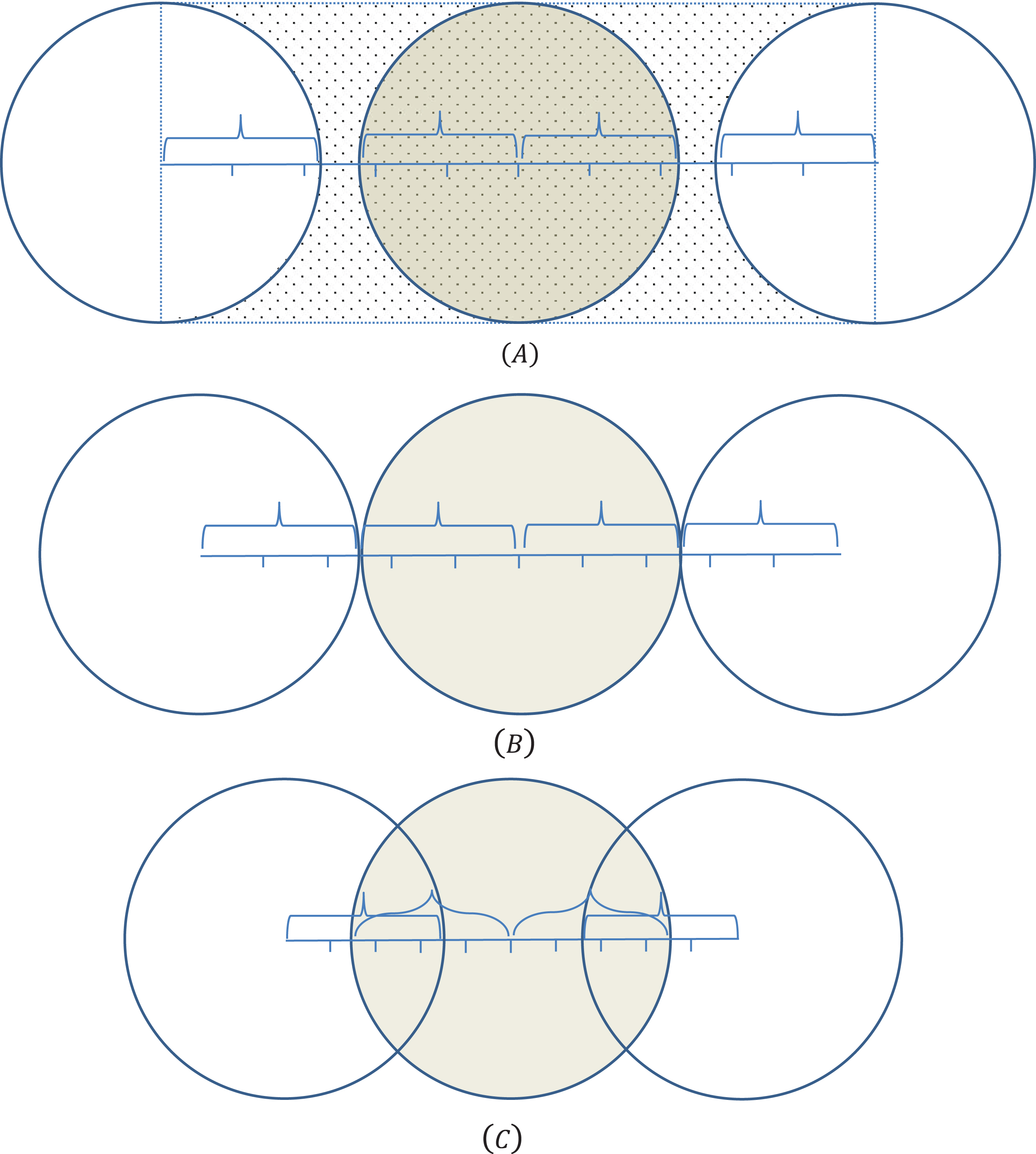
The p_a: for a = 0 to a = 10 when the distance between centers of clusters are (A) larger than, (B) equal to and (C) less than 4γ. The middle point is.

Fig. 2

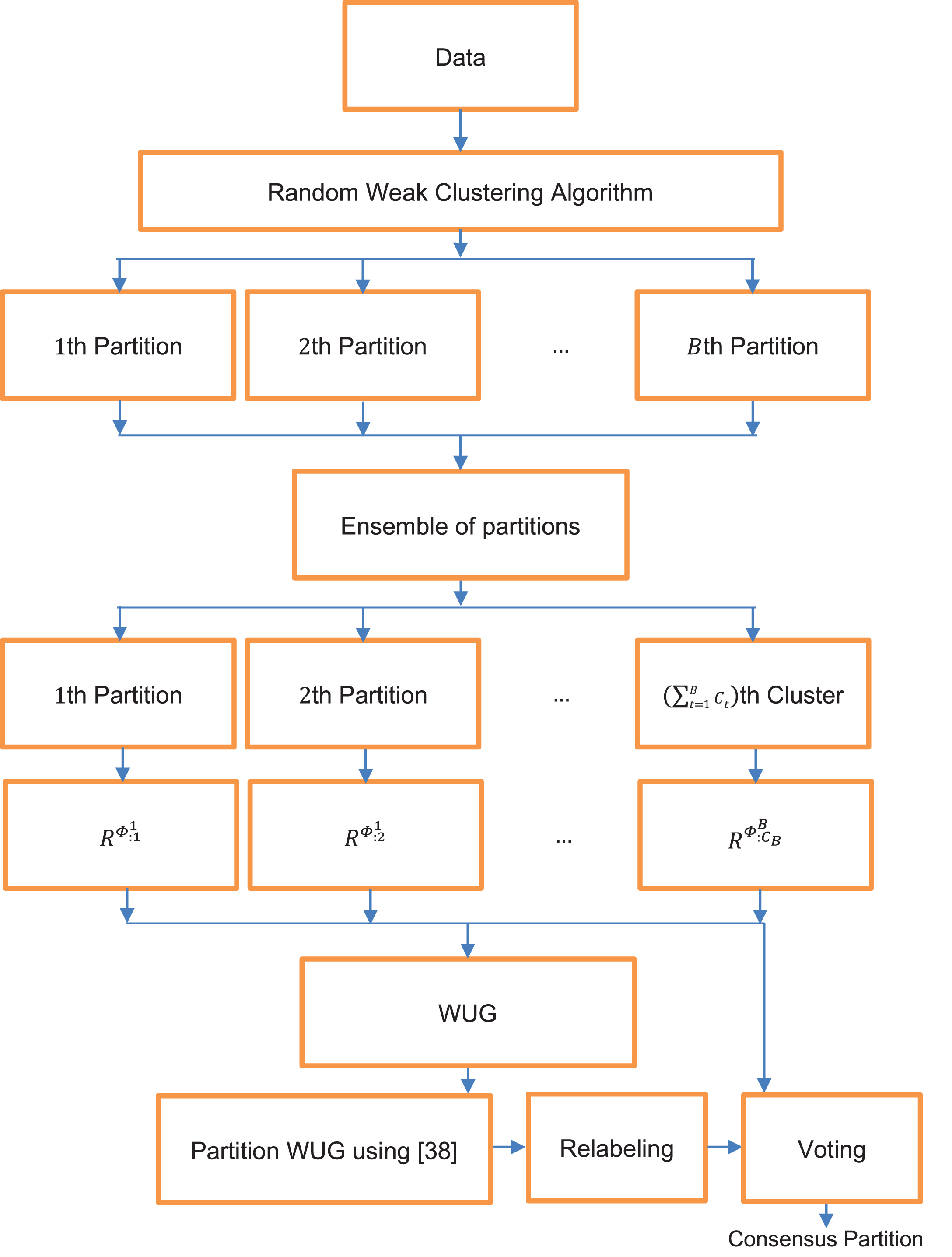
Block diagram of the proposed ensemble framework.

Considering the similarity criterion, a weighted un-directed graph (WUG) has been created that is represented by G ( Φ ) = (V ( Φ ) , E ( Φ )) for showing relationships between these clusters. According to the above graph G ( Φ ), V ( Φ ) stands for a set of vertices representing clusters in ensemble Φ . Hence, all vertices are considered a cluster in the ensemble Φ and E ( Φ ) refers to the edge weights between vertices; that is, clusters.

It is notable that the SIS between two clusters would be utilized as the weight of the edge connecting them; that is, weight would be computed based on Equation (12) so that the higher the SIS between them, the more probable they exhibit an equal cluster. Now we have a graph partitioning problem [38]. Hence, a partition of vertices in graph G ( Φ ) would be achieved designated by CC with dimension $\sum_{j = 1}^{B} C_{j} \times C$ . Thus, CC_ji = 1, if the $R^{Φ_{: q}^{p}}$ is a member of the ith consensus cluster in which $\sum_{i = 1}^{p - 1} C_{i} + q = j$ . Our aim has been to get this partitioning via minimization of an objective function in which the vertices have high similarity in the same sub-sets and have great difference from the vertices in other sub-sets. Thus, for solving the optimization problem, a normalized spectral clustering algorithm [39] has been utilized for obtaining a final partition of CC. Finally, vertices in the same sub-sets have been utilized for representing a cluster. Hence, a novel ensemble with the aligned clusters denoted by Λ has been defined by Equation (13). $Λ_{ir}^{k} = {\begin{matrix} 1 & (\sum_{t = 1}^{k - 1} C_{t} + j = p) ⋏ (R_{i}^{Φ_{: j}^{k}} = 1) ⋏ ({CC}_{pr} = 1) \\ 0 & o . w . \end{matrix}$ (13) In addition, time complexity for making the cluster relationship would be $O (| D_{: 1} | {(\sum_{t = 1}^{B} C_{t})}^{2})$ .

3.2.3 Consensus function

Following assurance of the ensemble of the aligned (or re-labeled) partitions out of the main ensemble of the partitions, Λ, where $Λ_{: :}^{k}$ represents a matrix of size |D_:1| × C for any k∈ { 1, 2, …, B }, would be available to extract the consensus partition. Based on the ensemble Λ, consensus function could be re-written by Equation (14). $π_{ij}^{*} = {\begin{matrix} 1 & \forall p \in {1, 2, \dots, C} : {\bar{Λ}}_{ij} ⩾ {\bar{Λ}}_{ip} \\ 0 & o . w . \end{matrix}$ (14) so that ${\bar{Λ}}_{ij} = \sum_{k = 1}^{B} Λ_{ij}^{k}$ . Moreover, time complexity of the consensus function is O (|D_:1|CB).

3.2.4 Time complexity

The whole complexity of the algorithm equals $O (| D_{: 1} | I (\sum_{t = 1}^{B} C_{t}) + | D_{: 1} | (\sum_{t = 1}^{B} C_{t}) + | D_{: 1} | {(\sum_{t = 1}^{B} C_{t})}^{2} + | D_{: 1} | CB)$ . As seen, time complexity has been linear proportionate with the number of the objects and thus for the ensemble learning, the higher the number of the base clusters; that is, $\sum_{t = 1}^{B} C_{t}$ , would not mean the better function of the ensemble. Hence, it is possible to control Equation $\sum_{t = 1}^{B} C_{t} ⪡ | D_{: 1} |$ and thus this new algorithm would be proper to address the large scale datasets. Nevertheless, based on the optimized computational conditions, supposing $\sum_{t = 1}^{B} C_{t} \approx \sqrt{| D_{: 1} |}$ , overall time complexity is $O ({| D_{: 1} |}^{\frac{3}{2}} I + {| D_{: 1} |}^{2})$ .

4 Experimental analysis

In this section, we conduct two experimentations using the proposed algorithm and present them on two subsections. First, we present our assessment metrics. Then, analysis of our method’s parameters is presented. After that, the first experimental subsection is presented where we compare our method with the traditional ensemble clustering algorithms. After that, the second experimental subsection is presented where we compare our method with the modern ensemble clustering algorithms.

4.1 Assessment metrics

To evaluate our method its efficacy is computed based on external metrics. We also present the consumed times by different methods. Notably, 2 external criteria are utilized for measuring similarities between the output cluster tags forecasted by various approaches and ground-truth cluster tags of the used data-sets. Assume that the partition like the ground-truth cluster tags of the data-set is designated by π^*. Therefore, Equation (15) defines the target partition π^*: $π_{ji}^{*} = {\begin{matrix} 1 & L_{D_{j :}} = i \\ 0 & L_{D_{j :}} \neq i \end{matrix}$ (15) here L_{D
_j:} stands for target tag of jth instance.

Assume we have 2 partitions defined on a data-set D; that is, φ^* (consensus partition) and π^* (a partition similar to the target tags of that data-set), values between φ^* and π^* could be as n_ij represents numbers of the similar data objects in cluster $π_{: i}^{*}$ and cluster $φ_{: j}^{*}$ . Moreover, Equation (10) defines the adjusted rand index (ARI):

$ARI (φ^{*}, π^{*}) = \frac{\sum_{i} \sum_{j} (\begin{matrix} n_{ij} \\ 2 \end{matrix}) - \frac{[\sum_{i} (\begin{matrix} n_{i -} \\ 2 \end{matrix}) \sum_{j} (\begin{matrix} n_{- j} \\ 2 \end{matrix})]}{(\begin{matrix} n \\ 2 \end{matrix})}}{\frac{1}{2} [\sum_{i} (\begin{matrix} n_{i -} \\ 2 \end{matrix}) + \sum_{j} (\begin{matrix} n_{- j} \\ 2 \end{matrix})] - \frac{[\sum_{i} (\begin{matrix} n_{i -} \\ 2 \end{matrix}) \sum_{j} (\begin{matrix} n_{- j} \\ 2 \end{matrix})]}{(\begin{matrix} n_{- -} \\ 2 \end{matrix})}}$ (16) where n_ij indicates the number of objects shared between ith cluster in φ^* and jth cluster in π^*, n_i- indicates the number of objects in ith cluster of partition φ^*, n_-j indicates the number of objects in jth cluster of partition π^*, and n_-- is number of total objects. Table 3 reports the variables. In addition, Equation (17) defines the normalized mutual information (NMI) [86]. $NMI (φ^{*}, π^{*}) = \frac{2 \sum_{i} \sum_{j} n_{ij} \log \frac{n_{ij} n}{n_{i -} n_{- j}}}{\sum_{ij} n_{i -} \log \frac{n_{i -}}{n_{- -}} - \sum_{j} n_{- j} \log \frac{n_{- j}}{n_{- -}}}$ (17)

Therefore, the more the partition φ^* (consensus partition) as well as the partition π^* (the partition similar to the target tags of data-set) have similarity to each other, the higher these metrics.

4.2 Parameter analysis

Here, some adjustments would be provided for diverse ensemble clustering algorithms for ensuring their reproducibility.

Therefore, number of the clusters in all base partitions would be randomly adjusted in the introduced ensemble clustering algorithm in which kmeans clustering algorithm has been applied for producing their primary partitions. Actually, in all traditional and advanced clustering algorithms, number of the clusters in each base primary partition of the ensemble would be given as a prior information and k-means clustering algorithm would be employed for generating their primary partitions. To set parameter γ in our ensemble method, we set B to 10 and make an experimental analysis in Fig. 3 for Iris [87] and Wine [87] data-sets. The results presented by Fig. 3-a indicate that the best value for γ is 0.5. Therefore, we use 0.5 for variable γ from now on. By setting the parameter γ to 0.5, we have about 100 clusters in our ensemble according to Fig. 3-b. Freezing the parameter γ at 0.5, we perform a similar experimental analysis in Fig. 4 for different values of parameter B. The results presented by Fig. 4 indicate that the best value for B is 20. However, parameter B would be always 20 from now on. Therefore, for the compared methods, their parameters have been determined on the basis of their researchers’ recommendations. Finally, quality of the clustering algorithms would be expressed as the average over 50 independent runs.

Fig. 3

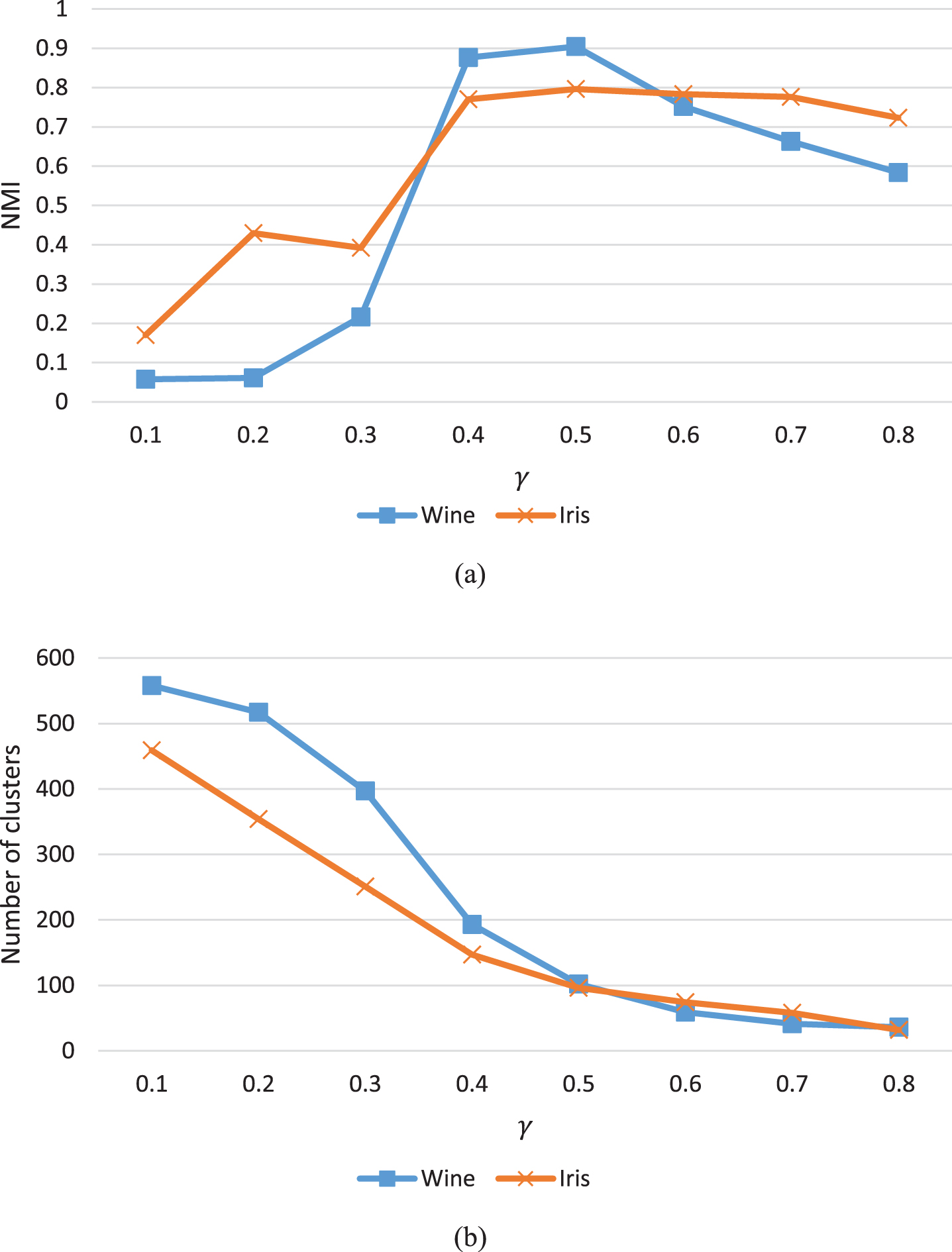
(a) The performance of our method on Iris and Wine data-sets in terms of NMI for different γ values when B is 10. (b) The number of formed clusters in our ensemble method for different γ values when B is 10.

Fig. 4

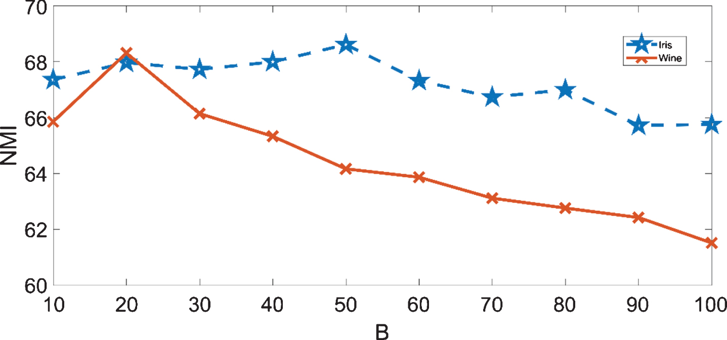
The performance of our method on Iris and Wine data-sets in terms of NMI for different B values when γ is 0.5.

All data-sets are first normalized according to Equation (18). ${\dot{D}}_{ji} = \frac{(D_{ji} - min_{k \in {1, \dots, F}} D_{jk})}{max_{k \in {1, \dots, F}} D_{jk} - min_{k \in {1, \dots, F}} D_{jk}}$ (18) where ${\dot{D}}_{ji}$ is the ith normalized attribute in the jth object.

4.3 Analysis of traditional ensembles

4.3.1 Benchmark data-sets

Experimental evaluations have been performed on 8 benchmark data-sets. These data-sets are: Ring, Banana, Aggregation, Imbalance, Iris, Wine, Breast, and Digits with respectively 1500, 2000, 788, 2250, 150, 178, 569, and 5620 objects and 3, 2, 7, 2, 3, 3, 2, and 10 clusters. The cluster distributions of the artificial 2D data-sets, i.e. Ring, Banana, Aggregation, Imbalance, have been shown in Fig. 5. The real-world data-sets are derived from the UCI data-set repository [87].

Fig. 5

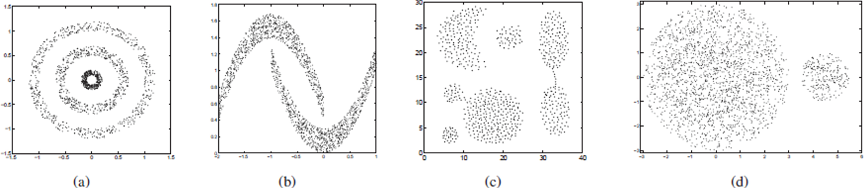
Scatter plot of four artificial data-sets: (a) Ring, (b) Banana, (c) Aggregation, and (d) Imbalance.

4.3.2 Compared traditional methods

For investigating this algorithm efficacy, a comparison has been made between the algorithm and the traditional ensemble clustering algorithms like the evidence accumulation clustering (EAC) along with the single-link clustering algorithm as the consensus function (EAC+SL), the average-link clustering algorithm as the consensus function (EAC+AL) [48], the weighted connection triple (WCT) along with the single-link clustering algorithm as the consensus function (WCT+SL), the average-link clustering algorithm as the consensus function (WCT+AL) [65], the weighted triple quality (WTQ) along with the single-link clustering algorithm as the consensus function (WTQ+SL), the average-link clustering algorithm as the consensus function (WTQ+AL) [65], the combined similarity measure (CSM) along with the single-link clustering algorithm as the consensus function (CSM+SL), the average-link clustering algorithm as the consensus function (CSM+AL) [65], the cluster-based Similarity Partitioning Algorithm (CSPA) [40], the HyperGraph Partitioning Algorithm (HGPA) [40], the Meta CLustering Algorithm (MCLA) [40], (11) the selective un-weighted voting (SUW) [54], (12) the selective weighted voting (SWV) [54], the expectation maximization (EM) [74], and finally the iterative voting consensus (IVC) [77].

Additionally, a comparison has been made between this new method and other strong base clustering algorithms like normal spectral clustering algorithm (NSC) [39], the density-based spatial clustering of the utilizations with noise algorithm (DBSCAN) [35], as well as the clustering by rapid search and find of the density peak algorithm (CFSFDP) [36]. It is notable that the comparison aims at testing if the introduced method would be a solid method or not.

Then, we applied a Gaussian kernel for the NSC algorithm and a value 0.1 × k where 1 ⩽ k ⩽ 20 has been selected as the kernel parameter, i.e. σ². Finally, the most acceptable partition obtained by changing the above parameters has been chosen to compare them.

It should be noted that both the CFSFDP and DBSCAN algorithms need the input parameter ɛ. Therefore, ɛ-value has been estimated with the average distance between each data point and the respective average point designated by $\bar{AD}$ . Nonetheless, all the algorithms possibly demand a given ɛ-value. Hence, all of them have been experimented by setting ɛ to value $\frac{\bar{AD}}{r}$ where r is an integer between 1 to 10. Changing ɛ to different values results in different partitions and finally the most acceptable partition has been applied to make the comparisons.

To describe other methods, we initially employ kmeans clustering algorithm 1000 times with different initializations over a given data-set D. For each partition, a random integer number in interval $[2; \sqrt{| D_{: 1} |}]$ is produced as the number of clusters in that partition. Therefore, we produce a pool of 1000 partitions over the given data-set D. Then, to computed the performance of ensemble method Y, we consider the ensemble size recommended by that method in its corresponding paper for the value of parameter B (if it does not recommend any specific number, we will use 20 for the value of parameter B). Then, we randomly select B partitions from the pool as their ensemble and apply the method on it. After that, the NMI value of the resultant partition with the ground truth labels is computed and stored as ${NMI}_{D}^{Y} (1)$ . After that, we compute ${NMI}_{D}^{Y} (i)$ for 2 ⩽ i ⩽ 50. Finally, the ${NMI}_{D}^{Y}$ (where ${NMI}_{D}^{Y} = \frac{\sum_{i = 1}^{50} {NMI}_{D}^{Y} (i)}{50}$ ) is reported as the performance of method Y on data-set D in terms of NMI metric.

4.3.3 Experimental results

In this subsection, we initially utilized diverse consensus functions for extracting the final partitions. It is notable that it is necessary to have an edited EAC (EEAC) for applying EAC on some ensembles [88, 89]. Also, we applied the model introduced in Part 3.4 as a distinct consensus function for the extraction of the final partition out of the output graph of Algorithm 1. Figures 6 and 7 schematically represents the experimental outputs of distinct ensemble clustering techniques on diverse data-sets with regard to ARI metric (and NMI metric). According to the analyses, this new consensus function introduced in Part 3.4 has been considered to be the most acceptable method followed by the EEAC+SL consensus function. As demonstrated, MCLA and EEAC+AL consensus functions have been the 3rd and 4th ones. Hence, this new mechanism introduced in Part 3.4 has been viewed as the dominant consensus function.

Fig. 6

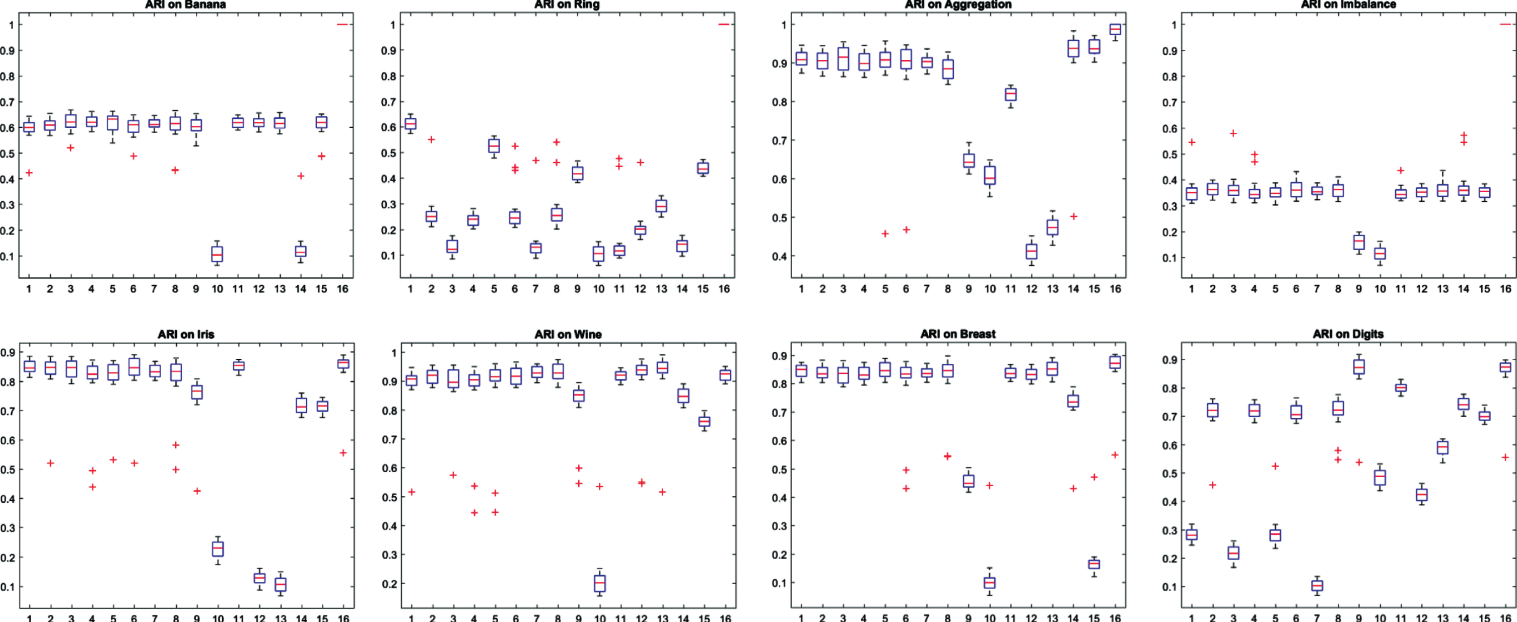
Experimental results of different ensemble methods on different data-sets in terms of ARI. EAC+SL, EAC+AL, WCT+SL, WCT+AL, WTQ+SL, WTQ+AL, CSM+AL, CSM+SL, CSPA, HGPA, MCLA, SUV, SWV, EM, IVC and proposed methods are respectively methods 1–16.

Fig. 7

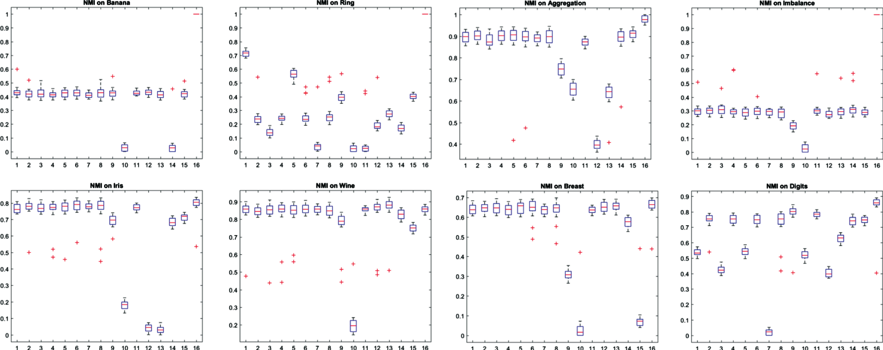
Experimental results of different ensemble methods on different data-sets in terms of NMI. EAC+SL, EAC+AL, WCT+SL, WCT+AL, WTQ+SL, WTQ+AL, CSM+AL, CSM+SL, CSPA, HGPA, MCLA, SUV, SWV, EM, IVC and proposed methods are respectively methods 1–16.

Considering ARI and NMI metrics, Figs. 6 and 7 compare efficacies of diverse ensemble clustering algorithms on the artificial as well as the real-world data-sets. According to Figs. 6 and 7, this new ensemble clustering algorithm increases clustering accuracy in both of the synthetic and the real-world data-sets in comparison with other available ensemble clustering algorithms in terms of ARI metric (and NMI metric). Based on the experimental outputs, this algorithm could efficiently recognize or identify diverse clusters and enhance the functionalities of the traditional ensemble clustering algorithms.

4.4 Analysis of modern ensembles

4.4.1 Benchmark data-sets

Used data-sets include Semeion, Multiple-Features, Image-Segmentation, Forest-CoverType, MNIST, Optical-Digit-Recognition, Landsat-Satellite, ISOLET, USPS, Letter-Recognition, Breast-Cancer, Bupa, Glass, Galaxy, SAHeart, IonoSphere, Iris, Wine, and Yeast respectively with 1,593, 2,000, 2,310, 3,780, 5,000, 5,620, 6,435, 7,797, 11,000, 20,000, 683, 345, 214, 323, 462, 351, 150, 178, 1,484 instances and respectively with 10, 10, 7, 7, 10, 10, 6, 26, 10, 26, 2, 2, 6, 7, 2, 2, 3, 3, 10 numbers of real target clusters. All data-sets are from UCI data-set repository [87] except data-set MNIST [90] and data-set USPS [91].

4.4.2 Modern ensemble methods

In the current subsection section, our ensemble will be compared to some of the state-of-the-art methods. The methods comparing to our methods include H[ybrid B[i-P[artite G[raph F[ormulation (HB-PGF) [67], Ensemble of Locally Reliable Clusters (ELRC) [73], Sim-Rank Similarity (S-RS) [92], W [eighted C[onnected T[riple (W-CT) [65], C [luster S [election E [vidence A [ccumulation C [lustering (CS-EAC) [93, 94], W [eighted E [vidence A [ccumulation C[lustering (W-EAC) [95], W [isdom of C [rowds E [nsemble (WCE) [96], G [raph P [artitioning with M [ulti-G [ranularity L [ink A [nalysis (GPM - GLA) [95], T [wo-level co-association M [atrix E [nsemble (TME) [97], E [lite C [luster S [election E [vidence A [ccumulation C [lustering (ECS-EAC) [89], and Average Linkage Second Diversity Measure (ALSDM) [29, 98].

To describe the setting, we again employ kmeans clustering algorithm 1000 times with different initializations over a given data-set D. For each partition, a random integer number in interval $[2; \sqrt{| D_{: 1} |}]$ is produced as the number of clusters in that partition. Therefore, we produce a pool of 1000 partitions over the given data-set D. Then, to computed the performance of ensemble method Y, we consider the ensemble size recommended by that method in its corresponding paper for the value of parameter B (if it does not recommend any specific number, we will use 20 for the value of parameter B). Then, we randomly select B partitions from the pool as their ensemble and apply the method on it. After that, the FM value of the resultant partition with the ground truth labels is computed and stored as ${FM}_{D}^{Y} (1)$ . After that, we compute ${FM}_{D}^{Y} (i)$ for 2 ⩽ i ⩽ 50. Finally, the ${FM}_{D}^{Y}$ (where ${FM}_{D}^{Y} = \frac{\sum_{i = 1}^{50} {FM}_{D}^{Y} (i)}{50}$ ) is reported as the performance of method Y on data-set D in terms of FM metric.

4.4.3 Experimental analysis

Comparison of the proposed ensemble method with the different modern ensemble ones, which are presented in Part 4.4.2, for different data-sets presented in Part 4.4.1 in terms of ARI metric is depicted in Fig. 8. It is notable that result of each method on each data-set is an average of 50 independent trials here. We assume that the ARI value of each method on different datasets is a variable, we perform a Friedman test on the results presented by Fig. 8. The P-value is about 0.01 that there is a significant difference between the variables. The post hoc analysis indicates most of this difference comes from the ALSDM and our algorithm with a P-value of about 0.041.

Fig. 8

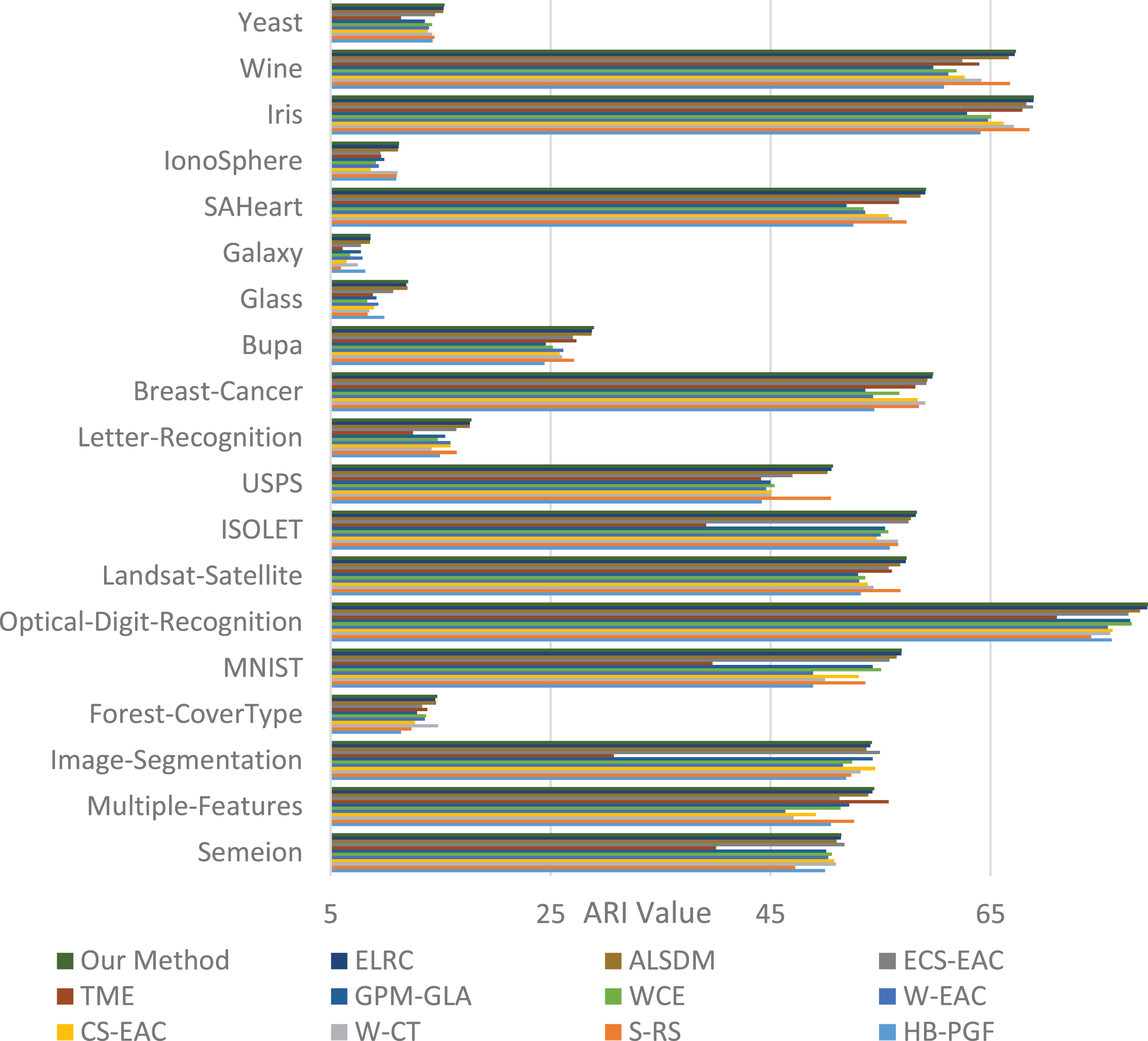
Comparison of the proposed ensemble method with the different modern ensemble ones in terms of ARI. Horizontal axis depicts the ARI value.

Figure 9 depicts the consumed time of the different algorithms in terms of the number of instances. We used KDD-CUP99 data-set with 1048576 instances and 2 clusters here. It is obvious that our method is not the best, but it is still more scalable than most of the state of the art ensemble methods.

Fig. 9

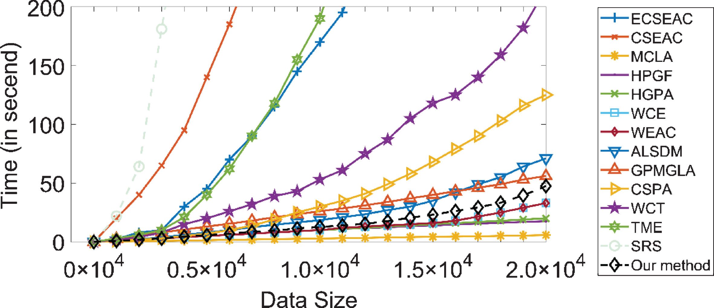
The consumed time analysis of the different algorithms in terms of the number of instances.

5 Conclusion and future works

As the basic clustering algorithm k-means clustering algorithm is extensively regarded as a low-computational algorithm, it has been regarded as a poor clustering method as several variables influenced their performance that includes improper selection of the initial cluster centers and dissimilar data distribution. Therefore, the present research aimed at introducing one of the novel ensemble clustering algorithms with the multiple kmeans clustering algorithm. This new ensemble clustering method enjoys benefits of kmeans clustering algorithm including its low computation and great speed but it has important disadvantage like incapability of detecting the nonspherical and nonuniform clusters. Actually, our ensemble clustering algorithm could enhance quality and stability of kmeans clustering algorithm and it is proved that aggregation of multiple poor partitions would be more acceptable than or equal to a strong partition. The research also tried for solving each ensemble clustering problem via describing the valid local clusters. Moreover, the research called data surrounding a cluster center in kmeans clustering as the valid local data clusters. Therefore, for generating distinct clustering, a duplicate approach of the production of the poor clustering results; namely, the use of the kmeans clustering algorithm as the base clustering algorithm has been utilized on the nonappeared data in the formerly valid local clusters. Hence, empirical analyses compared this new ensemble clustering algorithm with multiple available ensemble clustering algorithms and 3 strong basic clustering algorithms running on a series of artificial and the real-world bench-mark data-sets. Based on the empirical outputs, this ensemble clustering algorithm outperformed the advanced ensemble clustering procedures. Furthermore, effectiveness of our ensemble clustering algorithm has been investigated with the result of its suitability to address the large-scale data-sets.

Compliance with ethical standards

Conflict of interest

The authors declare that they have no conflict of interest.

Ethical approval

This article does not contain any studies with human participants or animals performed by any of the authors.

Footnotes

Acknowledgments

Research results of 2017 general topic “classroom teaching evaluation research based on core literacy” (Project No.: cd-db17207) of the 13th Five-year Plan of Beijing Education Science.

References

Jamalinia

, Khalouei

, Rezaie

, Nejatian

, Bagheri-Fard

and Parvin

, Diverse classifier ensemble creation based on heuristic dataset modification, Journal of Applied Statistics 45(7) (2018), 1209–1226.

Parvin

, Alinejad-Rokny

, Minaei-Bidgoli

and Parvin

, A new classifier ensemble methodology based on subspace learning, J Exp Theor Artif Intell 25(2) (2013), 227–250.

Tavana

, Parvin

and Rezazadeh

, Parkinson detection: an image processing approach, Journal of Medical Imaging and Health Informatics 7(2) (2017), 464–472.

Shabaniyan

, Parsaei

, Aminsharifi

, Movahedi

M.M.

, Jahromi

A.T.

, Pouyesh

and Parvin

, An artificial intelligence-based clinical decision support system for large kidney stone treatment, Australasian Physical & Engineering Sciences In Medicine 42(3) (2019), 771–779.

Aminsharifi

, Irani

, Pooyesh

, Parvin

, Dehghani

, Yousofi

, Fazel

and Zibaie

, Artificial neural network system to predict the postoperative outcome of percutaneous nephrolithotomy, Journal of Endourology 31(5) (2017), 461–467.

Omidvar

M.N.

, Nejatian

, Parvin

and Rezaie

, A new natural-inspired continuous optimization approach, Journal of Intelligent & Fuzzy Systems (2018), 1–17.

Yasrebi

, Eskandar-Baghban

, Parvin

and Mohammadpour

, Optimisation inspiring from behaviour of raining in nature: droplet optimisation algorithm, International Journal of Bio-Inspired Computation 12(3) (2018), 152–163.

Alishvandi

, Gouraki

G.H.

and Parvin

, An enhanced dynamic detection of possible invariants based on best permutation of test cases, Computer Systems Science And Engineering 31(1) (2016), 53–61.

Nejatian

, Omidvar

, Mohamadi

, Baghbani

A.E.

, Rezaie

and Parvin

, An optimization algorithm based on behavior of see-see partridge chicks, Journal of Intelligent & Fuzzy Systems 33(6) (2017), 3227–3240.

10.

Mao

and Hou

, Object-based forest gaps classification using airborne LiDAR data[J], Journal of Forestry Research 30(2) (2019), 617–627.

11.

Sutrisno

, Windiastuti

, Octaviani

, et al., A feasibility study of seabed cover classification standard in generating related geospatial data[J], Geo-spatial Information Science 22(4) (2019), 304–313.

12.

Han

and Kamber

, Data Mining: Concepts and Techniques, Morgan Kaufmann (2001).

13.

Jenghara

M.M.

, Ebrahimpour-Komleh

, Rezaie

, Nejatian

, Parvin

and Syed-Yusof

S.K.

, Imputing missing value through ensemble concept based on statistical measures, Knowledge and Information Systems 56(1) (2018), 123–139.

14.

Shamshirband

, Amini

, Anuar

N.B.

, Kiah

M.L.M.

, Teh

Y.W.

and Furnell

, D-FICCA: A density-based fuzzy imperialist competitive clustering algorithm for intrusion detection in wireless sensor networks, Measurement 55 (2014), 212–226.

15.

Agaian

Sos

, Madhukar

Monica

and Chronopoulos

Anthony T.

, A new acute leukaemia-automated classification system, Computer Methods in Biomechanics and Biomedical Engineering: Imaging & Visualization, 6 (2018), 303–314, DOI: 10.1080/21681163.2016.1234948

16.

Khoshnevisan

, Rafiee

, Omid

, Mousazadeh

, Shamshirband

and Hamid

S.H.A.

, Developing a fuzzy clustering model for better energy use in farm management systems, Renewable and Sustainable Energy Reviews 48 (2015), 27–34.

17.

Jenghara

M.M.

, Ebrahimpour-Komleh

and Parvin

, Dynamic protein–protein interaction networks construction using firefly algorithm, Pattern Analysis and Applications 21(4) (2018), 1067–1081.

18.

Hosseinpoor

M.J.

, Parvin

, Nejatian

and Rezaie

, Gene Regulatory Elements Extraction in Breast Cancer by Hi-C Data Using a Meta-Heuristic Method, Russian Journal of Genetics 55(9) (2019), 1152–1164.

19.

Nejatian

, Rezaie

, Parvin

, Pirbonyeh

, Bagherifard

and Yusof

S.K.S.

, An innovative linear unsupervised space adjustment by keeping low-level spatial data structure, Knowledge and Information Systems 59(2) (2019), 437–464.

20.

Pirbonyeh

, Rezaie

, Parvin

, Nejatian

and Mehrabi

, A linear unsupervised transfer learning by preservation of cluster-and-neighborhood data organization, Pattern Analysis and Applications 22(3) (2019), 1149–1160.

21.

Moradi

, Nejatian

, Parvin

and Rezaie

, CMCABC: Clustering and memory-based chaotic artificial bee colony dynamic optimization algorithm, International Journal of Information Technology & Decision Making 17(04) (2018), 1007–1046.

22.

Parvin

, Nejatian

and Mohamadpour

, Explicit memory based ABC with a clustering strategy for updating and retrieval of memory in dynamic environments, Applied Intelligence 48(11) (2018), 4317–4337.

23.

Nejatian

, Parvin

and Faraji

, Using sub-sampling and ensemble clustering techniques to improve performance of imbalanced classification, Neurocomputing 276 (2018), 55–66.

24.

Parvin

, Mirnabibaboli

and Alinejad-Rokny

, Proposing a classifier ensemble framework based on classifier selection and decision tree, Eng Appl Artif Intell 37 (2015), 34–42.

25.

Jain

A.K.

and Dubes

R.C.

, Algorithms for Clustering Data. Prentice Hall, (1988).

26.

Jain

A.K.

, Data clustering: 50 years beyond K-means, Pattern Recognition Letters 31(8) (2010), 651–666.

27.

MacQueen

J.B.

, Some methods for classification and analysis of multivariate observations, Proc. of 5-th Berkeley Symposium on Mathematical Statistics and Probability, Berkeley, University of California Press 1 (1967), 281–297.

28.

Nazari

, Dehghan

, Nejatian

, Rezaie

and Parvin

, A Comprehensive Study of Clustering Ensemble Weighting Based on Cluster Quality and Diversity, Pattern Anal Appl 22(1) (2019), 133–145.

29.

Najafi

, Parvin

, Mirzaie

, Nejatian

and Rezaie

, Dependability-based cluster weighting in clustering ensemble, Stat Anal Data Min: The ASA Data Sci Journal (2020), 1–14. https://doi.org/10.1002/sam.11451.

30.

Abbasi

, Nejatian

, Parvin

, Rezaie

and Bagherifard

, Clustering ensemble selection considering quality and diversity, Artif Intell Rev 52(2) (2019), 1311–1340.

31.

Mojarad

, Parvin

, Nejatian

and Rezaie

, Consensus Function Based on Clusters Clustering and Iterative Fusion of Base Clusters, Fuzziness and Knowledge-Based Systems 27(1) (2019), 97–120.

32.

Bagherinia

, Minaei-Bidgoli

, Hossinzadeh

and Parvin

, Elite fuzzy clustering ensemble based on clustering diversity and quality measures, Applied Intelligence 49(5) (2019), 1724–1747.

33.

Mojarad

, Nejatian

, Parvin

and Mohammadpoor

, A fuzzy clustering ensemble based on cluster clustering and iterative Fusion of base clusters, Applied Intelligence 49(7) (2019), 2567–2581.

34.

Likas

, Vlassis

and Verbeek

, The global fc-means clustering algorithm, Pattern Recognition 35(2) (2003), 451–461.

35.

Ester

, Kriegel

, Sander

and Xu

, A density-based algorithm for discovering clusters in large spatial databases with noise, In Evangelos Simoudis, Jiawei Han, Usama M. Fayyad. Proceedings of the Second International Conference on Knowledge Discovery and Data Mining (KDD-96), AAAI Press, (1996), pp. 226–231.

36.

Rodriguez

and Laio

, Clustering by fast search and find of density peaks, Science 344(6191) (2014), 1492–1496.

37.

Karypis

, Han

E.-H.S.

and Kumar

, Chameleon: a hierarchical clustering algorithm using dynamic modeling, IEEE Computer 32(8) (1999), 68–75.

38.

Shi

and Malik

, Normalized cuts and image segmentation, IEEE Transactions on Pattern Analysis and Machine Intelligence 22(8) (2000), 888–905.

39.

A.Y.

, Jordan

M.I.

and Weiss

, On Spectral Clustering: Analysis and an Algorithm, in: T.G. Dietterich, S. Becker, Z. Ghahramani (Eds.), Advances in Neural Information Processing Systems 14 MIT Press, Cambridge, MA, (2002).

40.

Strehl

and Ghosh

, Cluster ensembles: a knowledge reuse framework for combining multiple partitions, Journal on Machine Learning Research 3 (2002), 583–617.

41.

Gionis

, Mannila

and Tsaparas

, Clustering aggregation, ACM Transactions on Knowledge Discovery from Data 1 (1) (2007), 1–30.

42.

Zhou

, Ensemble Methods: Foundations and Algorithms, CRC Press, (2012).

43.

Iam-On

and Boongoen

, Comparative Study Of Matrix Refinement Approaches For Ensemble Clustering, Machine Learning 98 (2015), 269–300.

44.

Parvin

, Beigi

and Mozayani

, A clustering ensemble learning method based on the ant colony clustering algorithm, Int J Appl Comput Math 11(2) (2012), 286–302.

45.

Parvin

, Minaei-Bidgoli

, Alinejad-Rokny

and Punch

W.F.

, Data weighing mechanisms for clustering ensembles, Comput Electr Eng 39(5) (2013), 1433–1450.

46.

Alizadeh

, Minaei-Bidgoli

and Parvin

, To improve the quality of cluster ensembles by selecting a subset of base clusters, J Exp Theor Artif Intell 26(1) (2014), 127–150.

47.

Alizadeh

, Minaei-Bidgoli

and Parvin

, Optimizing Fuzzy Cluster Ensemble in String Representation, IJPRAI 27(2) (2013).

48.

Fred

and Jain

, Combining multiple clusterings using evidence accumulation, IEEE Transactions on Pattern Analysis and Machine Intelligence 27(6) (2005), 835–850.

49.

Kuncheva

and Vetrov

, Evaluation of stability of k-means cluster ensembles with respect to random initialization, IEEE Transactions on Pattern Analysis and Machine Intelligence 28(11) (2006), 1798–1808.

50.

Zhang

, Jiao

, Liu

, Bo

and Gong

, Spectral clustering ensemble applied to SAR image segmentation, IEEE Transactions on Geoscience and Remote Sensing 46(7) (2008), 2126–2136.

51.

Law

, Topchy

and Jain

, Multi-objective data clustering, Proc. IEEE Conf. Computer Vision and Pattern Recognition, (2004).

52.

, Chen

, You

, et al., Hybrid fuzzy cluster ensemble framework for tumor clustering from bio-molecular data, IEEE/ACM Transactions on Computational Biology and Bioinformatics 10(3) (2013), 657–670.

53.

Fischer

and Buhmann

, Bagging for path-based clustering, IEEE Transactions on Pattern Analysis and Machine Intelligence 25(11) (2003), 1411–1415.

54.

Zhou

and Tang

, Clusterer ensemble, Knowledge-Based Systems 19(1) (2006), 77–83.

55.

Hong

, Kwong

, Wang

and Ren

, Resampling-based selective clustering ensembles, Pattern Recognition Letters 41(9) (2009), 2742–2756.

56.

Fern

and Brodley

, Random projection for high dimensional data clustering: A cluster ensemble approach, Proc. International Conference on Machine Learning (2003).

57.

Zhou

, Du

, Shi

, Wang

, et al., Learning a robust consensus matrix for clustering ensemble via Kullback-Leibler divergence minimization, Proc. the 25th International Joint Conference on Artificial Intelligence, (2015).

58.

, Li

, Liu

, et al., Adaptive noise immune cluster ensemble using affinity propagation, IEEE Transactions on Knowledge and Data Engineering 27(19) (2015), 3176–3189.

59.

Gullo

and Domeniconi

, Metacluster-based projective clustering ensembles, Machine Learning 98(1-2) (2013), 1–36.

60.

Yang

and Jiang

, Hybrid Sampling-Based Clustering Ensemble with Global and Local Constitutions, IEEE Transactions on Neural Networks and Learning Systems 27(5) (2016), 952–965.

61.

Topchy

, Minaei-Bidgoli

and Jain

, Adaptive clustering ensembles, Proc. the 17th International Conference on Pattern Recognition, (2004).

62.

Minaei-Bidgoli

, Parvin

, Alinejad-Rokny

, Alizadeh

and Punch

W.F.

, Effects of resampling method and adaptation on clustering ensemble efficacy, Artif Intell Rev 41(1) (2014), 27–48.

63.

Fred

and Jain

A.K.

, Data clustering using evidence accumulation, Proc. the 16th International Conference on Pattern Recognition (2002), 276–280.

64.

Yang

and Chen

, Temporal data clustering via weighted clustering ensemble with different representations, IEEE Transactions on Knowledge and Data Engineering 23(2) (2011), 307–320.

65.

Iam-On

, Boongoen

, Garrett

and Price

, A link-based approach to the cluster ensemble problem, IEEE Transactions on Pattern Analysis and Machine Intelligence 33(12) (2011), 2396–2409.

66.

Iam-On

, Boongoen

, Garrett

and Price

, A link-based cluster ensemble approach for categorical data clustering, IEEE Transactions on Knowledge and Data Engineering 24(3) (2012), 413–425.

67.

Fern

and Brodley

, Solving cluster ensemble problems by bipartite graph partitioning, Proc. of the 21st International Conference on Machine Learning (2004).

68.

Huang

, Lai

and Wang

C.D.

, Ensemble clustering using factor graph, Pattern Recognition 50 (2016), 131–142.

69.

Selim

and Ertunc

, Combining multiple clusterings using similarity graph, Pattern Recognition 44(3) (2011), 694–703.

70.

Boulis

and Ostendorf

, Combining multiple clustering systems, Proc. European Conf. Principles and Practice of Knowledge Discovery in Databases, (2004).

71.

Hore

, Hall

L.O.

and Goldgo

, A scalable framework for cluster ensembles, Pattern Recognition 42(5) (2009), 676–688.

72.

Long

, Zhang

and Yu

P.S.

, Combining multiple clusterings by soft correspondence, Proc. the 4th IEEE International Conference on Data Mining, (2005).

73.

Niu

, Khozouie

, Parvin

, Alinejad-Rokny

, Beheshti

and Mahmoudi

M.R.

, An Ensemble of Locally Reliable Cluster Solutions, Applied Sciences (2020).

74.

Topchy

, Jain

and Punch

, Clustering ensembles: Models of consensus and weak partitions, IEEE Transactions on Pattern Analysis and Machine Intelligence 27(12) (2005), 1866–1881.

75.

Wang

, Shan

and Banerjee

, Bayesian cluster ensembles, Statistical Analysis and Data Mining 4(1) (2011), 54–70.

76.

, Xu

and Deng

, A cluster ensemble method for clustering categorical data, Information Fusion 6(2) (2005), 143–151.

77.

Nguyen

and Caruana

, Consensus Clusterings, Proc. IEEE Intl Conf. Data Mining (2007), 607–612.

78.

Huang

, Extensions to the k-means algorithm for clustering large data sets with categorical values, Data Mining and Knowledge Discovery 2(3) (1998), 283–304.

79.

and Xia

, Zmproved Chameleon: A Lightweight Method for Identity Verification in Near Field Communication, 2016 International Symposium on Computer, Consumer and Control (IS3C), Xi’an, (2016), 387–392.

80.

Zhou

, Xu

and Liu

, Method for Determining the Optimal Number of Clusters Based on Agglomerative Hierarchical Clustering, in, IEEE Transactions on Neural Networks and Learning Systems 28(12) (2017), 3007–3017.

81.

Bezdek

J.C.

and Pal

N.R.

, Some new indexes of cluster validity, IEEE Transactions on Systems Man and Cybernetics Part B 28 (3) (1998), 301–315.

82.

Pal

N.R.

and Bezdek

J.C.

, On cluster validity for the fuzzy c-means model, IEEE Transactions on Fuzzy Systems 3(3) (1995), 370–379.

83.

Guha

, Rastogi

and Shim

, Cure: an efficient clustering algorithm for large databases, Proc. of the Conference on Management of Data (ACM SIGMOD) (1998), 73–84.

84.

Sneath

P.H.A.

and Sokal

R.R.

, Numerical Taxonomy, Freeman, San Francisco, London, (1973).

85.

King

, Step-wise clustering procedures, Journal of the American State Association 69 (1967), 86–101.

86.

T. S. A. V. W. T. Press, W. H. and Flannery

B. P.

, Conditional Entropy and Mutual Information. Numerical Recipes: The Art of Scientific Computing (3rd ed.). New York: Cambridge University Press., (2007).

87.

UCI Machine Learning Repository, http://www.ics.uci.edu/mlearn/ML- Repository.html, (2016).

88.

Parvin

and Minaei-Bidgoli

, A clustering ensemble framework based on elite selection of weighted clusters, Adv. Data Analysis and Classification 7(2) (2013), 181–208.

89.

Parvin

and Minaei-Bidgoli

, A clustering ensemble framework based on selection of fuzzy weighted clusters in a locally adaptive clustering algorithm, Pattern Anal Appl 18(1) (2015), 87–112.

90.

LeCun

, Bottou

, Bengio

and Haffner

, Gradient-based learning applied to document recognition, Proceedings of the IEEE 86(11) (1998), 2278–2324.

91.

Dueck

, Affinity propagation: Clustering data by passing messages, PhD dissertation, University of Toronto, (2009).

92.

Iam-On

, Boongoen

and Garrett

, Refining pairwise similarity matrix for cluster ensemble problem with cluster relations, in Proc. of International Conference on Discovery Science (ICDS), (2008), pp. 222–233.

93.

Alizadeh

, Minaei-Bidgoli

and Parvin

, Cluster ensemble selection based on a new cluster stability measure, Intelligent Data Analysis 18(3) (2014), 389–408.

94.

Alizadeh

, Minaei-Bidgoli

and Parvin

, A New Criterion for Clusters Validation, Artificial Intelligence Applications and Innovations (AIAI 2011, IFIP, Springer), Heidelberg, Part I, (2011), pp. 240–246.

95.

Huang

, Lai

J.H.

and Wang

C.D.

, Combining multiple clusterings via crowd agreement estimation and multi-granularity link analysis, Neurocomputing 170 (2015), 240–250.

96.

Alizadeh

, Yousefnezhad

and Minaei-Bidgoli

, Wisdom of Crowds cluster ensemble, Intell Data Anal 19(3) (2015), 485–503.

97.

Zhong

, Yue

, Zhang

and Lei

, A clustering ensemble: Two-level-refined co-association matrix with path-based transformation, Pattern Recognition 48(8) (2015), 2699–2709.

98.

Rashidi

, Nejatian

, Parvin

and Rezaie

, Diversity Based Cluster Weighting in Cluster Ensemble: An Information Theory Approach, Artif Intell Rev 52 (2) (2019), 1341–1368.