
Abstract
The importance of detecting faults in Unmanned Aerial Vehicles motivated researchers to work in this area over recent years. Complex relationships among UAV attributes (Sensor readings, and Commands) make the task a bit challenging. Many known algorithms consider detecting the faults by spotting data anomalies in the values of each attribute without concern for their context, which leaves an opportunity for potential improvement. The contextual faults occur when a defected sensor shows an invalid value concerning other attributes. Our contribution is a novel matrix platform for detecting the potential contextual faults. This platform consists of multiple small Decision Trees, instead of using one huge single Decision Tree, which could be difficult and time-consuming to produce, particularly in the case of a large dataset with too many attributes. We propose to use the C4.5 decision tree algorithm to build each decision tree. The Decision Tree is a machine learning technique, which is an effective supervised method used for classification. It is computationally inexpensive and capable of dealing with noisy data. Besides, our approach uses a sliding window technique during training and testing phases, which brings into consideration the effect of the previous state of the system on the process of detecting the contextual faults. The algorithm starts by collecting the attributes of the UAV into a table of pairs, where each pair consists of two attributes; then, it defines the Decision Tree matrix by assigning one Decision Tree for each pair of attributes. The Training step includes constructing training sub-datasets using the values of sliding windows. The C4.5 algorithm uses each constructed training sub-dataset to induce one Decision Tree in the matrix. Finally, the testing step is responsible for reading the values of the sliding windows and using the concerned Decision Tree to detect the contextual faults.
We evaluated our approach using Detection Rate, False Alarm Rate, Precision, and F1-score indicators. Moreover, we made a comparison with other broadly used algorithms, such as K-Means and One-Class SVM. Our approach showed superior results in detecting different types of faults (sensor-offset, sensor-stuck, sensor-drift, and sensor-cut). The DT-Matrix performance was neither affected by the small values of the outliers, nor by the number of the outliers, and this caused the DT-Matrix to work better in most of the experiments compared to the other algorithms.
Keywords
Introduction
The applications of the Unmanned Aerial Vehicles (UAV) have been increasing in recent years, including surveillance, reconnaissance, aerial photography, and disaster monitoring [1]. The UAV is a very complex system operated by Control, Aerodynamics, Communications, and Informatics ... The complexity of the UAV system raises the chances of its failure. During flight missions, the UAV sends channeled telemetry data to a ground station. The system collects the telemetry data and stores it in data rows on a fixed rate of periods. Each data row includes the values of the UAV attributes, which consist of the commands and the sensor readings. The commands could be the Altitude command, Rudder Command, Aileron Command..., while the sensor readings could be airspeed, pitch, roll, yaw ... . Anomaly detection algorithms predict system faults by finding patterns in data that do not conform to expected behavior [2]. These algorithms operate in three modes: [2, 3] Supervised, semi-supervised, and unsupervised. (1) The supervised anomaly detection algorithms assume the availability of training data with given labels for the normal class as well as for the anomalous class. (2) The semi-supervised anomaly detectors assume the training data has labeled instances for the normal class only. (3) The unsupervised anomaly detectors do not require any labeled training data, where they make the implicit assumption that normal instances are far more frequent than anomalies. UAV sensor faults can be classified into three types: point, contextual, and Collective [2]. A point fault means that the sensor gives an invalid or out of bounds value. A contextual fault occurs when the sensor shows an invalid value concerning the current context, such as a zero altitude value while the UAV being airborne. A collective fault means that the sensor shows a sequence of invalid values when put together collectively. For example, the UAV is climbing down, but the altimeter shows a fixed value [4]. Suppose the scenario, where the UAV is in a critical state on a low altitude, and the pilot decides to increase the altitude to save the UAV from crashing. If the pilot sends the proper altitude command to the UAV, but the response was unusually not effective, then the UAV will certainly crash. The previous scenario raises an issue about the pair: (Altitude command, Altitude sensor). Thus, we propose to analyze the values of each two attributes separately. An attributes pair consists of an effective attribute and a focused attribute. The focused attribute is associated with the potentially defected sensor, which we are trying to find. The effective attribute represents the context of the defect. In the previous scenario, the Altitude command is the effective attribute, and the Altitude sensor is the focused attribute. Our contribution includes a novel platform of Decision Tree Matrix (DT-Matrix) to detect the potential contextual faults. This platform produces multiple small Decision Trees instead of constructing a large single Decision Tree, which could be difficult and time-consuming, particularly for a large dataset with too many attributes. We propose to use the C4.5 Decision tree algorithm to generate each Decision Tree. Each Decision Tree in the DT-Matrix is responsible for detecting anomalies in the values of a pair of attributes. Another interesting point is using a sliding window technique, which brings into consideration the effect of the previous state of the system on the process of detecting the contextual faults. For each pair of attributes, we examine the observations of a sliding window [5]. The sliding window contains a limited number of previous values of the attributes of the concerned pair. Fig. 1 shows a block diagram of the proposed algorithm, where it starts by collecting the attributes of the UAV to form a table of attributes pairs; then, it builds the Decision Tree matrix by assigning one Decision Tree for each pair of attributes. The training step includes constructing new training sub-datasets using the values of a sliding window for each pair of attributes. The algorithm uses each generated training sub dataset to induce one Decision Tree in the matrix. In the testing step, our approach reads the values of a sliding window for each pair of attributes and uses the concerned Decision Tree to detect the contextual faults. We tested our approach on simulated flight datasets, and we compared our approach with other well-known algorithms such as K-Means and One-Class SVM. The DT-Matrix algorithm exhibited superior results in most of the experiments, in which it detected accurately sensor-offset, sensor-stuck, sensor-drift, and sensor-cut faults. In addition, it managed to define the faulty sensor and its context (the effective attribute). The rest of the paper is organized as follows. Section 2.0 provides a brief background and a review of related works. Problem description and our approach to using the C4.5 Decision tree Matrix are explained in section 3.0. We present the datasets, the results of experiments, a comparison with other algorithms, and the evaluation indicators in section 4.0. Finally, section 5.0 includes the conclusion and section 6.0 suggests the future work.
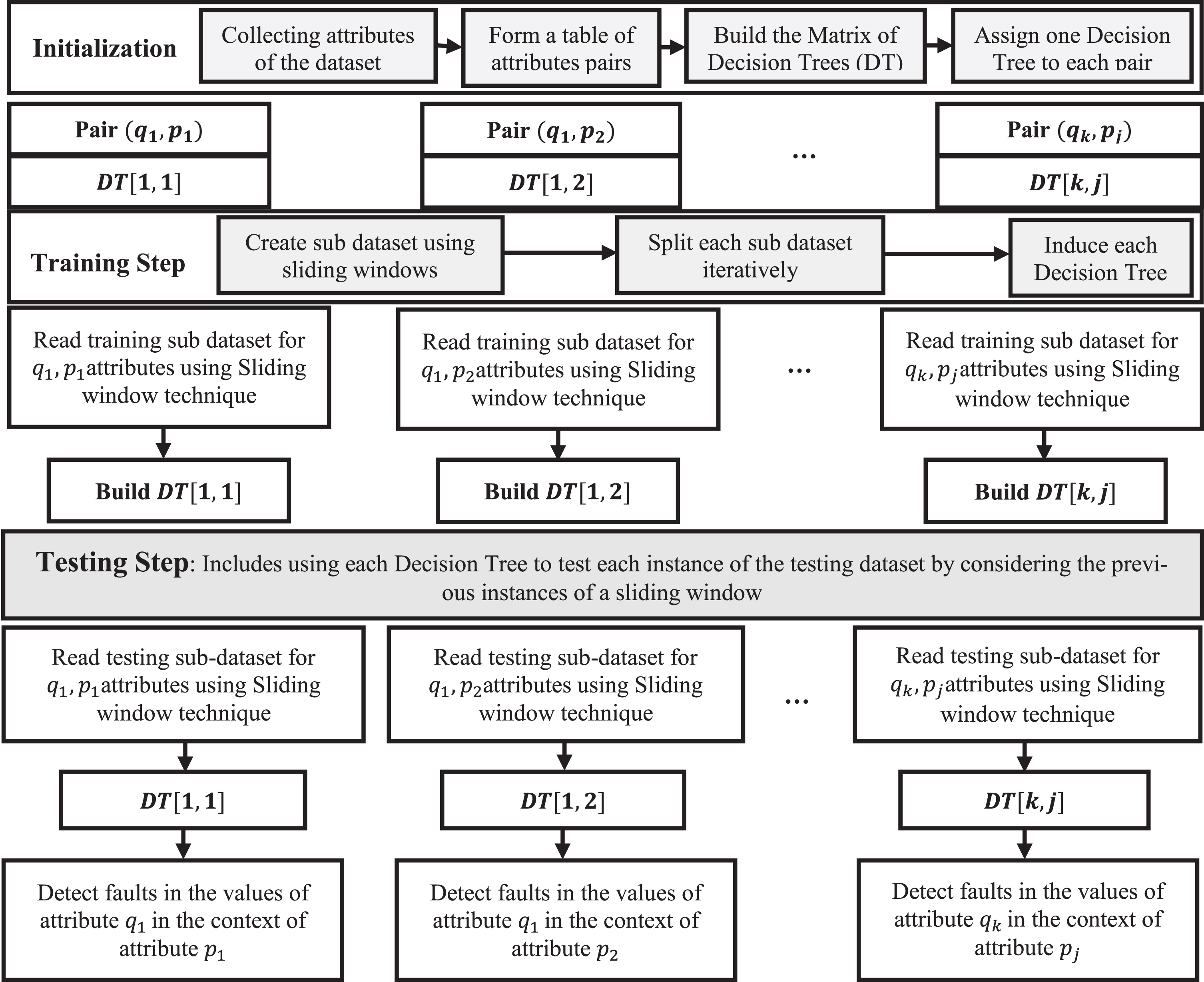
A block diagram of the DT-Matrix algorithm.
Over recent years, many researchers designed several algorithms to discover anomalies in order to detect system faults. There are three types of fault detection algorithms [6]: Model-based, Knowledge-based, and Data-driven-based algorithms. Cork et al. [7] used a model-based fault detection algorithm. They estimated the state of the UAV using a nonlinear dynamic model of the aircraft, in which they used the divergence of the estimated state from its actual value to detect system faults. The knowledge-based algorithms depend on predefined rules (if-then) sentences. Bu et al. [8] developed a UAV sensor fault detection method using a fuzzy logic model. The data-driven algorithms depend on the statistical information to detect outliers and label them as faults. Lin et al. [9] designed an online algorithm to detect UAV sensor faults based on a statistical analysis of sensor readings and navigation data. Khalastchi et al. [10], and Pokrajac et al. [11] used statistical methods to produce an anomaly score for each given point of the flight, where each anomaly score depends on a collection or a sliding window of monitored readings. These methods considered the point density, such as Mahalanobis Distance, or K-Nearest Neighbor (K - NN). Paffenroth et al. [12] developed a PCA-based anomaly detection algorithm to predict cyber-network attacks. Yong et al. [13] used kernel PCA to detect anomalies in the large datasets and complicated correlation of sensor data. Their proposed method detected the injected pulse and constant drift anomalies effectively. Lee et al. [14] used conventional time-series techniques to detect online anomalies, where they claimed that their method has better performance and accuracy than the deep-learning algorithm such as LSTM (Long Short Term Memory). However, their approach needed update in order to detect anomalies in multivariate datasets. On the other hand, Munir et al. [15] used a deep learning-based approach for anomaly detection in time series data. They claimed that their technique is accurate even in the detection of the small deviations in time series cycles, and is capable of detecting point and contextual anomalies in time series data even with periodic and seasonality characteristics. Tariq et al. [16] developed an anomaly detection method that depends on multivariate convolution LSTM with probabilistic PCA, where they claimed that their approach is 35.8% better in precision than the best baseline approaches. Most anomaly detection methods are based on fixed predefined limits, but in real-world systems, the data are often heterogeneous, noisy, and high dimensional. Hundman et al. [17] presented the capability of the dynamic error thresholding method to extract the abnormal flight points and LSTM for predicting spacecraft telemetry. Their method did not depend on unfamiliar labels or false parametric assumptions.
Anomaly detection is a classification problem, where classifiers tend to separate the abnormal from the normal instances. Alzubi et al. [18] developed a method for combining an ensemble of classifiers, where the outputs of multiple classifiers are weighted, and then the weighted outputs are summed to reach a single final classification decision. After comparing the outputs of all the classifiers, their approach adjusts the weights iteratively in order to converge to a final set of weights, and finally, the combined output reaches a consensus. Their results show improvement in the accuracy of the classification compared to the product and average methods. Decision tree (DT) is a classification algorithm that categorizes the data into predefined classes. It iteratively splits a training dataset, so as to construct a tree whose nodes contain instances of a single class. Pedro et al. [19] used DT to detect anomalies in cellular network data, where they used semi-synthetic data. Their approach correctly recognized more than 80% of the anomalous instances without false positives. Sugumaran [20], and Jian [8] used DT to build rules for a fault-diagnosis fuzzy classifier. However, they faced a limitation in performance due to the permanent rules in the fuzzy logic model, as it is not able to detect the unknown faults.
Methodology
In this section, we describe the problem, then we lay some definitions and explain the tools used to design the proposed approach.
Definitions
During each flight mission, the UAV streams large amounts of channeled data to a ground station. The system collects and stores the data in sequential rows. Each row contains the values of the UAV attributes. The attributes include the commands and the sensor readings. Let P = {p
j
: j < m} denotes the set of m focused attributes, and Q = {q
k
: k < n} be the set of n effective attributes. The recorded values of each pair of attributes (q
k
, p
j
) at time step t are
UAV Attributes pairs.
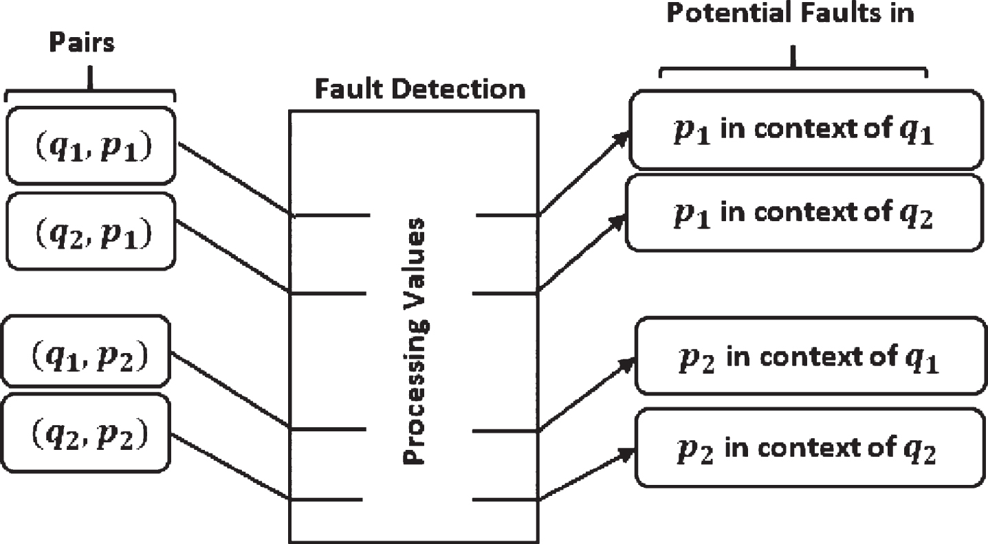
Detecting contextual faults using pairs of UAV attributes, where anomalies in the values of the pair (qk, pj) mean potential faults in the sensor pj in the context of qk values.
The Decision Tree (as a structure) is a tree-based knowledge representation used to characterize classification rules. It is easy to interpret, computationally inexpensive, and capable of dealing with noisy data [21] (Fig. 4 shows the structure of a decision tree). The Decision Tree machine learning technique is a powerful supervised method that generates a Decision Tree. The C4.5 algorithm is an improved and widely used learning technique for inducing small Decision Trees, and it is based on ID3 (Iterative Dichotomiser 3). C4.5 algorithm is composed of training data, testing data, heuristic evaluation functions, and a stopping criterion function. A tree induced with C4.5 consists of several branches, one root, and multiple nodes and leaves. Each node represents the current feature. A branch is a chain of nodes and arcs from root to a leaf [20]. The arcs are labeled with the possible values of the feature node from where they originate, and the leaves are labeled with the different classes (see Fig. 4).
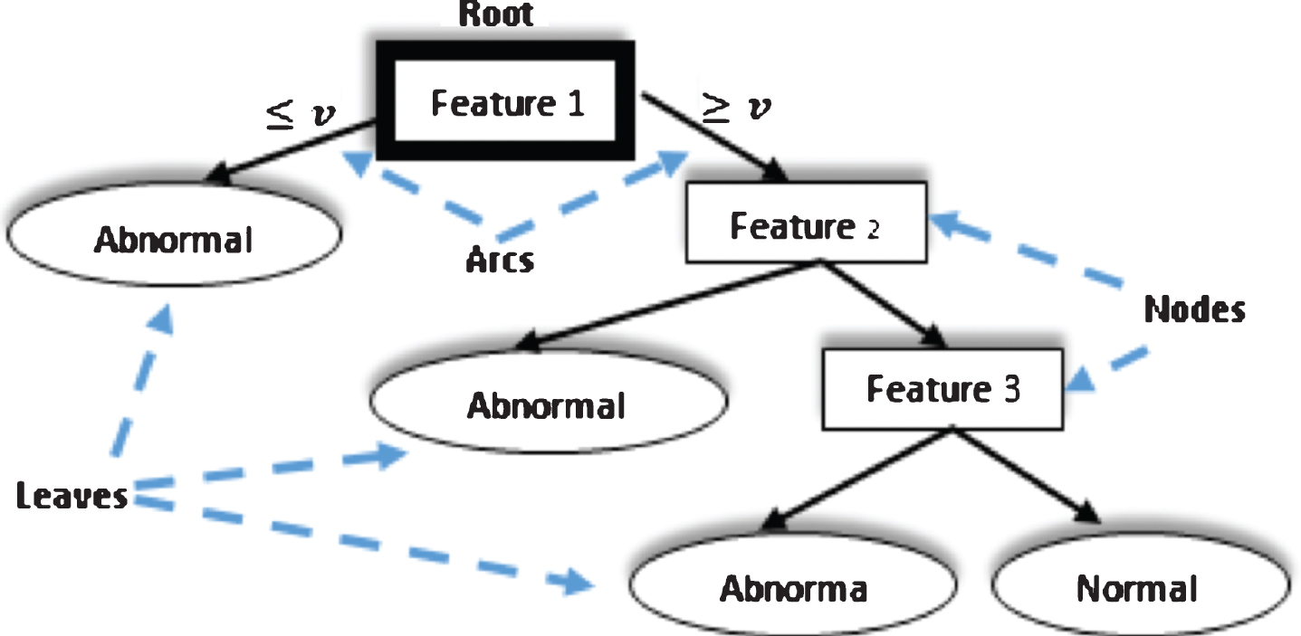
The structure of a Decision Tree.
The C4.5 uses Algorithm 1 to construct the tree, where it finds the best feature to split the training dataset S into subsets. For each subset, it creates a child node. The Algorithm recursively iterates until it reaches a pure set.
The pure subset means that all its rows are of one class (either abnormal or normal). A good Feature (A) is the one whose discriminating ability is high among the classes (its values do not vary much within a specified class, while it varies much among all the other classes) [20]. C4.5 algorithm selects the feature with the highest information gain g. The information gain is the expected reduction in entropy Ep. This reduction in entropy is caused by splitting the training dataset according to the given feature, which means that the information gain measures how well a given feature separates the training dataset giving their target classification. Information gain is defined as in Equation (1). The Entropy Ep is a measure of the disorder of the data, and it is calculated using Equations (2), (3) and (4),
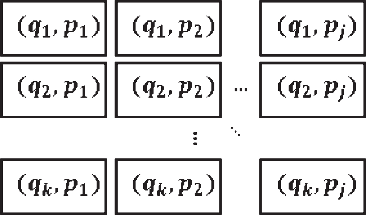
Algorithm 3 builds a matrix DT of (m × n) decision trees (see Fig. 5). m is the count of the effective attributes, and n is the count of the focused attributes. We assign a tree DT [k, j] to process the values of the pair (q
k
, p
j
) (refer to section 3.1). To construct the input for each tree, we use a sliding window of size h. The input at time step t for DT [k, j] is a vector
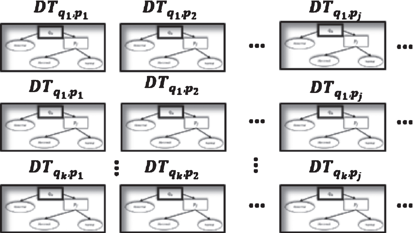
The matrix of Decision Trees.
The output of the tree DT [k, j] is the class of the point
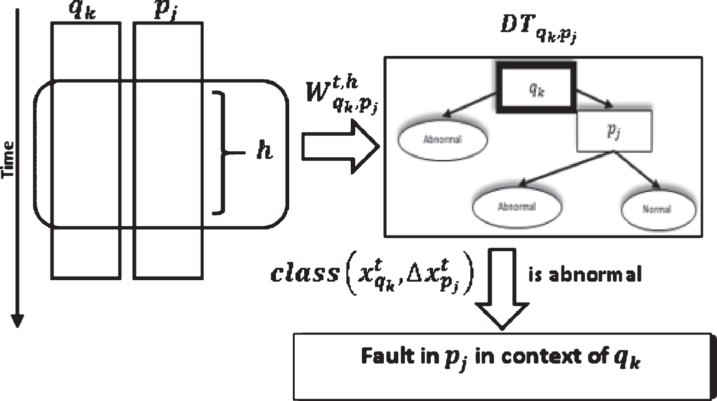
Detecting faults using C4.5 Decision Tree DT [k, j].
Datasets and setup
N. Oza [24] shared a dataset produced by NASA’s flight simulator “FLTz” for research purposes. “FLTz” is a simulator used to develop flight control, planning, and in-flight fault detection [25]. The “FLTz” dataset contains 20 flights for a fixed-wing aircraft. Each flight period ranges up to 40 minutes, and it is sampled at a rate of 1 Hz. The flights include all stages as takeoff, climb, cruise, and descent. Each flight consists of 36 attributes. To conduct our experiments, we chose only 18 attributes (see Table 1). We neglected the other attributes because their values were either constants, zeros, or identical to the values of other attributes, such as the identical commands of the right elevators and left elevators. The selected 18 attributes will be the effective attributes. The first 14 attributes are sensor readings, while the last four attributes are commands. We selected these first 14 attributes to be the focused attributes. Using these attributes, we extracted 238 pairs, where we neglected the pairs whose effective attribute is identical to the focused one, such as (Pitch, Pitch), (Airspeed, Airspeed) ...
The selected attributes of the FLTz flights
The selected attributes of the FLTz flights
To test our approach, we implemented a tool using C# programming language and Accord.net libraries. We evaluated our approach by comparing results with other anomaly-detection algorithms such as K-Means and One-class SVM. The K-Means algorithm is a clustering algorithm, which classifies a given data into K predefined categories. To use K-Means in anomaly detection, we set the value of K (the categories count) to be 1 class (The normal class) [26]. The abnormal points are the points that do not belong to the normal class.
K-means learns the centroid of the cluster from the training data, and for each test instance, the anomaly score is calculated using the distance to the normal class centroid. On the other hand, the One-Class SVM (Support Vector Machine) learns a region (a boundary) that contains the training data instances. If the test instance z falls within the learned region, then it is flagged as normal; otherwise, it is flagged as abnormal [2]. The One-Class SVM uses the output of a linear decision function to decide that the test instance z falls within the region [27]. The linear decision function is calculated using Equation (5),
We tested the algorithms for each pair of attributes on the same datasets, and we used the same input at each time step. The sliding window was of size h = 4 in all the experiments. We created eight datasets using the “FLTz” flights by combining some of the flights with each other. One of the datasets was the training dataset, which had 28510 rows. The other seven datasets were used for testing purpose and had 4593 rows each. Since The “FLTz” dataset does not have known faults, we seeded all the datasets by random sensor-offset, sensor-stuck, sensor-cut, and sensor-drift faults into different parameters such as (Pitch, Pitch Rate, Roll Rate, Yaw Rate, and airspeed). Table 2 shows the seven testing datasets and the ranges of the seeded offset faults for each faulty sensor. The offset faults mean that the sensor biases from its true value by a constant (see Figs. 7, 8 and 9). The stuck fault means that the reading of the sensor is trapped at a certain value (see Figs. 10 and 11). The drift fault means that the sensor shows increased values where it should not (see Fig. 12), and the cut fault means that the sensor recorded unusual zero values (see Fig. 13).
The testing Datasets
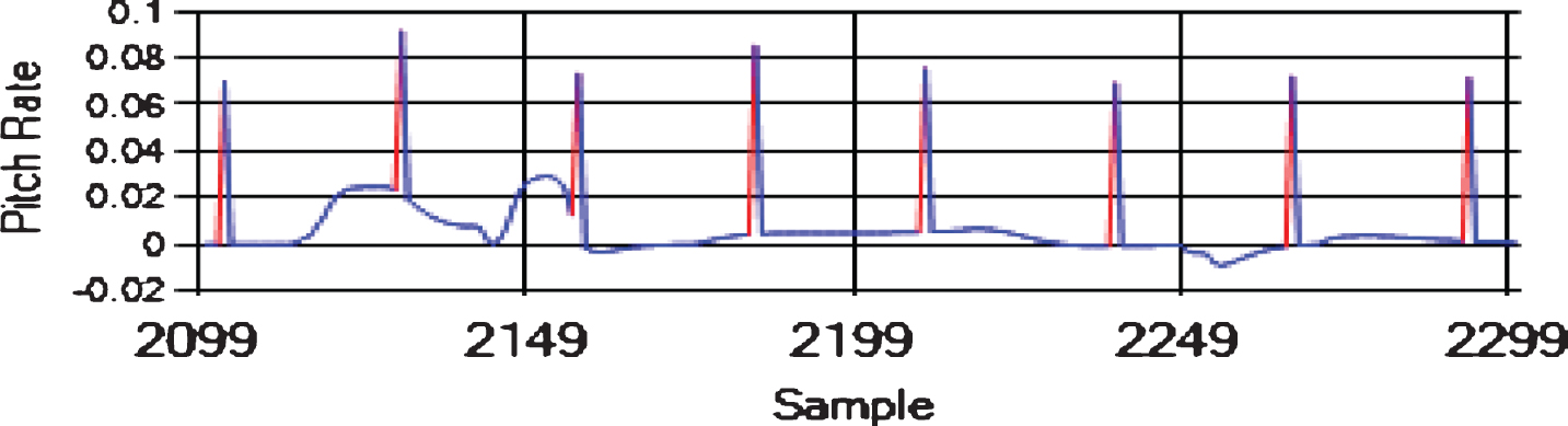
Sensor-offset faults in Pitch Rate (rad/s).
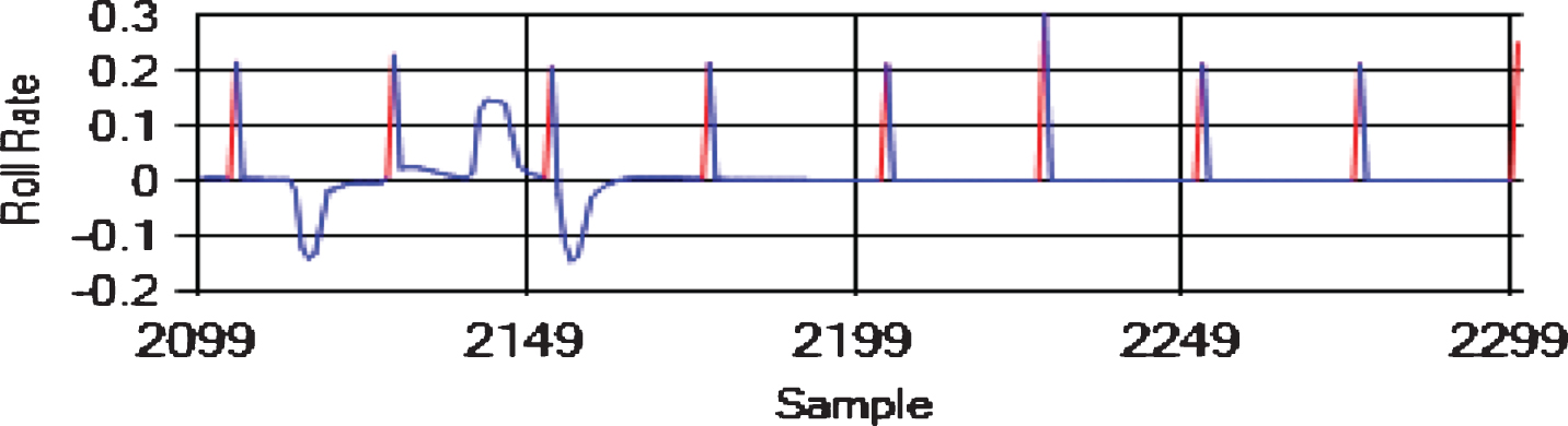
Sensor-offset faults in Roll Rate (rad/s).
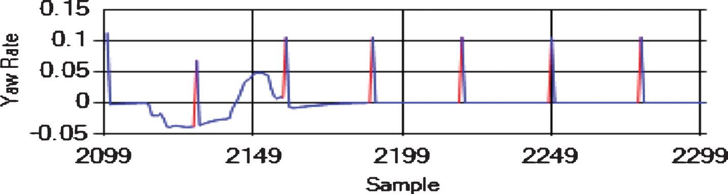
Sensor-offset faults in Yaw Rate (rad/s).
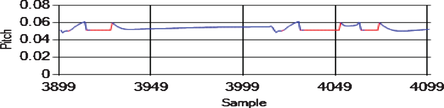
Sensor-stuck faults in pitch (rad).
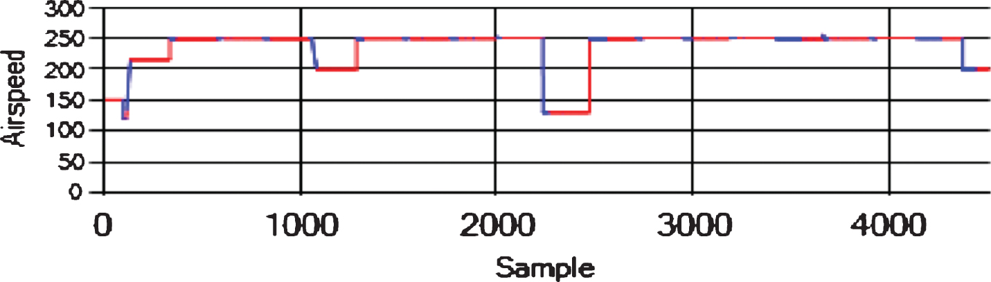
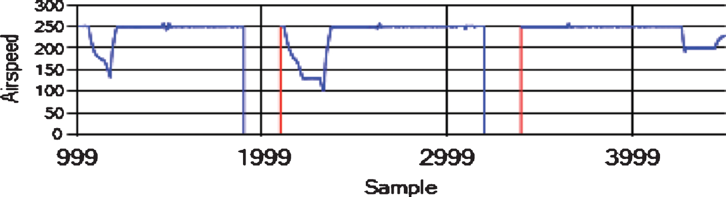
Sensor-stuck faults in airspeed (m/s).
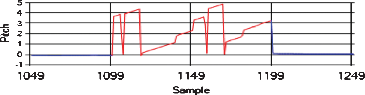
Sensor-drift faults in pitch (rad).
Sensor-cut faults in airspeed (m/s).
Four cases exist for the results of testing anomalies-detectors. (1) The True Positive (TP) refers to flagging the abnormal point as anomalous. (2) The False Positive (FP) refers to flagging the normal point as anomalous. (3) The True Negative (TN) refers to flagging the normal point as normal. (4) The False negative (FN) refers to flagging the abnormal point as normal. To evaluate the abnormal detection test, we use the Detection Rate (
Fault detection experiments
By using the previous indicators and the datasets DS1, DS2 ... , DS7 (see Table 2), we compared the efficiency of the three algorithms (DT-Matrix, K-Means, and One-Class SVM (see Table 3 and Table 4). To compare the efficiency of the anomaly detection algorithms, we need to consider into account the values of all the previous indicators altogether (refer to Section 4.2). Table 3 shows that the training time was the longest for the DT-Matrix algorithm, while Table 4 shows that the testing time was almost in the same range as the other algorithms. The DT-Matrix algorithm scored the best values for all indicators (see Table 4), in which the Detection Rate, Precision, and F1-Score had the highest values (near value one), and the False Alarm Rate had almost value zero. One-Class SVM algorithm results were convenient for detecting the sensor-offset faults in the datasets DS1, DS2, and DS3, but it failed to detect the Pitch sensor-stuck faults in dataset DS5. Moreover, its Detection rate dropped to almost zero in the case of sensor-drift, and sensor-cut faults in datasets DS6 and DS7. K-Means scored the worst values for all the indicators, and in most of the experiments (K-Means showed low Detection Rate, a considerable False Alarm, low Precision, and low F-Score).
Training time for DT-Matrix, K-Means, and One-Class SVM algorithms
Training time for DT-Matrix, K-Means, and One-Class SVM algorithms
Results of Testing DT-Matrix, K-Means, and One-Class SVM algorithms
The Precision of the compared algorithms varied greatly on the different datasets. One reason is the small range of the outliers compared to the range of the normal values on DS1, DS2, DS3, and DS4 (see Figs. 7–9 and 10), where a lot of normal instances were flagged as False Positive (FP) by K-Means algorithm, while DT-Matrix and One-Class SVM algorithms were more sensitive to these outliers, which had small values.
The reason for the sensitivity is the fixed classification rules of the generated Decision Trees and the concrete form of the linear decision function of the SVM. In DS4, which included sensor stuck faults, the precision of the K-Means increased, but the detection rate value stayed low, which means that the False Positive value decreased, while the True Positive value did not increase, causing similar bad results for K-Means algorithm. The precision indicator of the One-class SVM was high in DS4, DS5, DS6, and DS7, in where the faults were of continuous nature (sensor-stuck, sensor-cut, and sensor-drift), but the Detection rate was low, making the F-Score value very low too (see section 4.2), except for DS5, where it was difficult for SVM to separate the outliers from the normal instances. The reason is the increased number of outliers compared to the normal instances (see Figs. 10–12 and 13). Thus, the One-class SVM and the K-Means were less sensitive to the significant number of outliers in these datasets. All these results collectively indicate that the DT-Matrix algorithm was neither affected by the small values of the outliers, nor by the number of the outliers, and this caused the DT-Matrix algorithm to work better in most of the experiments compared to the One-class SVM, and the K-Means. Generally, the reliability of the Decision Tree algorithm depends significantly on the training dataset. Creating a training dataset needs to collect a sizeable real-life dataset for each UAV, collect all possible faults, and inject these faults into the training dataset. Usually, collecting a good training dataset is required for all similar supervised algorithms.
Through experiments, and by using a simple counting and mapping between attributes and anomalies, we noticed that the DT-Matrix algorithm proclaimed the context of the fault precisely, where it identified the faulty sensor, and its effective attributes accurately. The anomalies were detected using the values of the anticipated pairs of attributes (The context, and the faulty sensor). The results of the One-Class SVM algorithm were slightly similar in case of sensor-offset faults, while it was not suitable for detecting sensor-stuck, sensor-drift, and sensor-cut faults. K-Means algorithm failed in declaring the correct context of the detected faults, where the anomalies were detected in the values of the attributes that do not relate to the faulty sensor.
Fault detection is a crucial research area, specifically in complex systems like UAVs. We have proposed to use a matrix of decision trees (DT-Matrix) as an effective algorithm to detect anomalies in the flight data. Our approach is to apply the algorithm using pairs of UAV attributes, where we used the C4.5 machine learning technique to build a small and fast decision tree for each pair of attributes (Effective attribute, Focused attribute), with the help of sliding window technique. We compared our approach with other broadly used algorithms, such as K-Means and One-Class SVM. We used Detection rate, False alarm rate, precision, and F1-score as evaluation indicators. The DT-Matrix algorithm exhibited superior results in most of the experiments, where it managed to detect different types of faults (sensor-offset, sensor-stuck, sensor, drift, and sensor-cut) without being affected by the small values of the outliers, nor by the number of the outliers.
Future work
Future work includes enhancements to make the algorithm faster in training and testing phases. We can explore new methods for choosing the appropriate pairs of attributes in order to minimize the size of the processed values. Also, we can improve the split algorithm and the technique of finding the best splitting threshold. Moreover, we can use the matrix platform to test and compare other variants of decision tree algorithms, such as the Classification and Regression Trees (CART), Iterative Dichotomizer 3 (ID3), and the CHi-squared Automatic Interaction Detector (CHAID), or other machine learning algorithms such as LSTM (Long short memory networks) and logistic regression.
Footnotes
Acknowledgments
This work is supported by a grant from the Higher Institute for Applied Sciences and Technology, Damascus, Syria. The authors appreciate the valuable comments provided by the anonymous referees.