Certain types of m -polar interval-valued fuzzy graph

Abstract

In this paper, an unprecedented kind of fuzzy graph designated as m-polar interval valued fuzzy graph (m-PIVFG) is defined. Complement of the m-PIVFG open and closed neighborhood degrees of m-PIVFG are discussed. The other algebraic properties such as density, regularity, irregularity of the m-PIVFG are investigated. Moreover, some basic results on regularity and irregularity of m-PIVFG are proved. Free nodes and busy nodes of m-PIVFG is explored with some basic theorems and examples. Lastly, an application of m-PIVFG is described.

Abbreviations

Fuzzy set

Fuzzy graph

IVFS

Interval-valued fuzzy sets

IVFG

Interval-valued fuzzy graph

m-PFS

m-polar fuzzy sets

m-PFG

m-polar fuzzy graph

m-PIVFS

m-polar interval-valued fuzzy sets

m-PIVFG

m-polar interval-valued fuzzy graph

1 Introduction

Observing the vast application of graph theory which is a mathematical structure defined as an ordered pair G = (V, E) together with a set of vertices V and a set of edges E. A fuzzy model is needed to describe a fuzzy graph when there is a vagueness either in vertices or in edges or in both. Recently, applications of graph theory are mostly used in the fields of computer networks, electrical network, coding theory, operational research, architecture, data mining etc. In 1736 graph theoretical concept was first modeled by Swiss mathematician Euler from the concept of Konigsberg bridge problem.

For solving various decision making problems in real life fuzzy set, a non-empty set V together with a fuzzy set and a fuzzy relation have been applied. Ten years after Zadeh’s concept on fuzzy set in 1965, Kauffman [1] proposed the basic idea of fuzzy graph. Later Rosenfeld [2] developed this concept which have been successfully applied in information theory, modern science, engineering science, manufacturing, medical diagnosis, etc. In fact, he also detailed definition of several fuzzy concepts such as fuzzy vertex, edges, cycles, paths, connectedness, and so on. In 1994, Zhang [3, 4] gave the extension of the concept of fuzzy set and the idea of bipolar fuzzy sets. Mordeson and Peng [5 –7] incorporated the idea of complement fuzzy graph and demonstrated a few properties and operations on it. Later this concept was described by Sunitha and Kumar [8, 9].

In 2006, Nagoorgani and Chandrasekaran [10] studied on the degree of a node in fuzzy graph. Later on Shannon and Atanassov [11] elaborated the conceptualization of intuitionistic fuzzy relation and intuitionistic fuzzy graphs and described various properties. In 2008, Nagoorgani and Radha [12] introduced regular fuzzy graph which was later used to find density. In 2009, Hongmei and Lianhua [13] made a deeper study on IVFG, in 2011, Akram and Dudek [14] and in 2018 Rashmanlou et al. [15] studied some operations on it. Hawary [16] defined complete fuzzy graph and studied some new operations on it. Nagoorgani and Malarvizhu [17, 18] detailed isomorphic properties on fuzzy graphs and also gave the definition of the self-complementary fuzzy graphs. Then, Akram [19] presented the notations of bipolar fuzzy graphs and further researched on it [20, 52]. Later, the extension of bipolar fuzzy set and the idea of m-polar fuzzy sets (m-PFS) were introduced by Chen et al. [21] in 2014. Later on Rashmanlou briefly described categorical properties on it [22]. Samanta and Pal investigated on fuzzy tolerance graph [23], fuzzy threshold graph [24], fuzzy k-competition graphs [25], p-competition fuzzy graphs and also fuzzy planar graphs [26]. Some properties related to isomorphism and complement on IVFG were studied by Talebi and Rashmanlou [27]. Later, Ghorai and Pal [28, 29] described various properties on m-PFGs. They examined isomorphic properties on m-PFG. Ghorai and Pal [30] described the density of m-polar fuzzy graphs and some operations on it. Raut and Pal [31] studied on fuzzy permutation graph and its complements in 2018. Various extensions of fuzzy graphs [32] have been incorporated to handle the vagueness of the real world problem [33]. In this uncertain environment to solve various decision making problems [34], fuzzy graphs have used several models. Different types of research on generalized fuzzy graphs were discussed in [36 –42]. A through study on shortest path problem has made by Nayeem and Pal [51]. Some remarkable research studies regarding fuzzy graph are given in Table 1.

Table 1
Some remarkable research studies regarding fuzzy graphs.

References Contributions

Kauffman (1973) Introduction of fuzzy graphs

Rosenfeld (1975) Modification the concept of fuzzy graphs given by Kauffman (1973)

Sunitha (2001) New definition of complement of fuzzy graphs

Akram (2011) Interval-valued fuzzy graph

Akram &Dudek (2011) Bipolar fuzzy graphs

Samanta &Pal (2011) Fuzzy tolerance graph

Samanta &Pal (2011) Fuzzy threshold graph

Nagorgoni &Radha (2012) Regular fuzzy graph

Samanta &Pal (2013) Fuzzy k-competition graph and p-competition graph

Samanta &Pal (2014) Fuzzy planar graph

Ghorai &Pal (2015) m-polar fuzzy graph

Ghorai &Pal (2016) m-polar fuzzy planar graphs

Raut, Pal &Ghorai (2018) Fuzzy permutation graph and its complements

This study Balanced m-PIVFG with busy and free nodes, and their examples

References	Contributions
Kauffman (1973)	Introduction of fuzzy graphs
Rosenfeld (1975)	Modification the concept of fuzzy graphs given by Kauffman (1973)
Sunitha (2001)	New definition of complement of fuzzy graphs
Akram (2011)	Interval-valued fuzzy graph
Akram &Dudek (2011)	Bipolar fuzzy graphs
Samanta &Pal (2011)	Fuzzy tolerance graph
Samanta &Pal (2011)	Fuzzy threshold graph
Nagorgoni &Radha (2012)	Regular fuzzy graph
Samanta &Pal (2013)	Fuzzy k-competition graph and p-competition graph
Samanta &Pal (2014)	Fuzzy planar graph
Ghorai &Pal (2015)	m-polar fuzzy graph
Ghorai &Pal (2016)	m-polar fuzzy planar graphs
Raut, Pal &Ghorai (2018)	Fuzzy permutation graph and its complements
This study	Balanced m-PIVFG with busy and free nodes, and their examples

The main contribution of this study are as follows:

Concept of m-PIVFGs and complement of m-PIVFGs are introduced with examples.

Open and closed neighbourhood degree of a vertex of m-PIVFG are defined.

Definitions of regularity and irregularity in m-PIVFG and their examples.

Investigation of busy and free nodes and their examples.

Results on busy and free nodes.

The rest of the article is arranged as follows: Section 1 describes historical backgrounds of FSs, FGs, m-PFGs and IVFGs. Our aim and motivation are also written in this section. In section 2, some preliminary concepts regarding FGs, m-PFGs, IVFGs are described. Section 3 discussed about m-PIVFG and complement of m-PIVFG. In section 4, open and closed neighbourhood degree of a vertex of m-PIVFG are defined. Balanced m-PIVFG, regular m-PIVFG and also density of an m-PIVFG are also investigated and supported with examples. Some theorems related to these definitions are discussed with their proofs. In section 5, we define the irregularity of an m-PIVFGs with examples and some theorems with their proofs. Section 6 demonstrated the definition of busy nodes, free nodes with the help of examples and some basic theorems related to these. Section 7 is based on a summary of this article along with future works.

2 Preliminaries

In this part of this paper we briefly study some basic terminologies of FS, FGs, m-PFS and m-PFGs which are used in this paper. The basic definition of IFGs are also demonstrated.

Fuzzy sets, extension of the classical notion of the set were proposed by Zadeh [43] in 1965. A fuzzy set is a set of elements having degrees of membership. A fuzzy set A = (S, m) is a pair of set S and a membership function m : S → [0, 1]. Throughout this article, we use the notation G^* as a classical graph and G as a graph defined in a fuzzy environment.

Definition 2.1. ([21]) An m-PFS (or a [0, 1] ^m-set) on a set X is a function A : X → [0, 1] ^m. The collection of all m-PFS on X is addressed as m (X).

Definition 2.2. [44] Let A be an m-PFS on X. An m-polar fuzzy relation on A is an m-PFS B of X × X such that B (x, y) ≤ min {A (x) , A (y)} ∀x, y ∈ X i.e. for each i = 1, 2, . . . , m and ∀x, y ∈ X p_i ∘ B (x, y) ≤ min {p_i ∘ A (x) , p_i ∘ A (y)}, where p_i means membership value of ith pole.

Definition 2.3. [44] An m-PFG of a crisp graph G^* = (V, E) is a pair G = (A, B) where A : V → [0, 1] ^m is an m-PFS in V and B : V × V → [0, 1] ^m is an m-PFS in V × V such that for each i = 1, 2, . . . , m; p_i ∘ B (xy) ≤ min {p_i ∘ A (x) , p_i ∘ A (y)} ∀xy ∈ V × V and B (xy) =0 ∀xy ∈ (V × V) - E, where 0 = (0, 0, . . . , 0) is the smallest element in [0, 1] ^m. A and B are known as the m-polar fuzzy vertex set and edge set of G, respectively.

Definition 2.4. [45] An IVFS A on V is defined as $A = {(x, [μ_{A}^{l} (x), μ_{A}^{u} (x)]) : x \in V}$ , where $μ_{A}^{l} (x)$ and $μ_{A}^{u} (x)$ are fuzzy subsets on V such that $μ_{A}^{l} (x) \leq μ_{A}^{u} (x)$ , ∀x ∈ V.

Based on this set a graph called IVFG is defined.

Definition 2.5. [13] By an IVFG of a crisp graph G^* = (V, E) we mean G = (A, B), where $A = [μ_{A}^{l} (x), μ_{A}^{u} (x)]$ is an IVFS on V and $B = [μ_{B}^{l} (xy), μ_{B}^{u} (xy)]$ is an IVFS on edge set E, such that $μ_{B}^{l} (xy) \leq min {μ_{A}^{l} (x), μ_{A}^{l} (y)}$ , $μ_{B}^{u} (xy) \leq min {μ_{A}^{u} (x), μ_{A}^{u} (y)}$ ∀xy ∈ E.

Definition 2.6. [46] An m-PIVFG of a graph G^* = (V, E) is a pair G = (V, A, B) consists of a non-empty set V together with pair of interval-valued function A : V → [0, 1] ^m is an m-PFS in V and B : V × V → [0, 1] ^m and μ : V × V → [0, 1] ^m for each i = 1, 2, . . . , m; $p_{i} \circ μ_{A} (x) = [p_{i} \circ μ_{A}^{l} (x), p_{i} \circ μ_{A}^{u} (x)]$ , $0 \leq μ_{A}^{l} (x) \leq μ_{A}^{u} (x) \leq 1$ and $p_{i} \circ μ_{B} (xy) = [p_{i} \circ μ_{B}^{l} (xy), p_{i} \circ μ_{B}^{u} (xy)]$ , $0 \leq μ_{B}^{l} (xy) \leq μ_{B}^{u} (xy) \leq 1$ and for every i, the interval number of a vertex x and of an edge xy in G satisfying $p_{i} \circ μ_{B}^{l} (xy) \leq p_{i} \circ min {μ_{A}^{l} (x), μ_{A}^{l} (y)}$ , $p_{i} \circ μ_{B}^{u} (xy) \leq p_{i} \circ min {μ_{A}^{u} (x), μ_{A}^{u} (y)}$ , ∀x, y ∈ V.

Definition 2.7. [46] Let G = (V, A, B) of G^* = (V, E) be an m-PIVFG. The complement $\bar{G}$ of G is an m-PIVFG $\bar{G} = (\bar{A}, \bar{B})$ , where $p_{i} \circ μ_{\bar{B}} (xy) = [p_{i} \circ μ_{\bar{B}}^{l} (xy), p_{i} \circ μ_{\bar{B}}^{u} (xy)]$ , $p_{i} \circ μ_{\bar{B}}^{l} (xy) = min {p_{i} \circ μ_{A}^{l} (x), p_{i} \circ μ_{A}^{l} (y)} - p_{i} \circ μ_{B}^{l} (xy)$ , and $p_{i} \circ μ_{\bar{B}}^{u} (xy) = min {p_{i} \circ μ_{A}^{u} (x), p_{i} \circ μ_{A}^{u} (y)} - p_{i} \circ μ_{B}^{u} (xy)$ for every i and x, y ∈ V.

Lots of works have been done on this graph [47 –50]. In the following section balanced m-PIVFG, regularity m-IVFG are defined with suitable examples. Some theorems related to regularity of m-IVFG are also discussed.

3 Balanced m-PIVFG

Herein, the concept of neighbourhood of m-PIVFG are introduced and demonstrated with examples. Also, in this part we described balanced and regularity of m-PIVFG with appropriate examples and some theorems related to these are also explained with their proofs.

Definition 3.1. Let G = (V, A, B) be an m-PIVFG of a crisp graph G^* = (V, E). The open-neighbourhood degree of a vertex x in G is defined by $\deg (x) = ([p_{1} \circ {deg}_{μ}^{l} (x), p_{1} \circ {deg}_{μ}^{u} (x)], [p_{2} \circ {deg}_{μ}^{l} (x), p_{2} \circ {deg}_{μ}^{u} (x)], . . ., [p_{i} \circ {deg}_{μ}^{l} (x), p_{i} \circ {deg}_{μ}^{u} (x)], . . ., [p_{m} \circ {deg}_{μ}^{l} (x), p_{m} \circ {deg}_{μ}^{u} (x)])$ , for i = 1, 2, . . . , m where $p_{i} \circ {deg}_{μ}^{l} (x)$ and $p_{i} \circ {deg}_{μ}^{u} (x)$ is defined by $p_{i} \circ {deg}_{μ}^{l} (x) = \sum_{y \in N (x)} p_{i} \circ μ_{B}^{l} (xy)$ and $p_{i} \circ {deg}_{μ}^{u} (x) = \sum_{y \in N (x)} p_{i} \circ μ_{B}^{u} (xy)$ , for every i. Moreover, $p_{i} \circ μ_{B}^{l} (xy) > 0$ , $p_{i} \circ μ_{B}^{u} (xy) > 0$ , for xy ∈ E and $p_{i} \circ μ_{B}^{l} (xy) = 0$ , $p_{i} \circ μ_{B}^{u} (xy) = 0$ , for xy ∉ E, x, y ∈ A.

Definition 3.2. Let G = (V, A, B) be an m-PIVFG of a crisp graph G^* = (V, E). If all the vertices have a similar open-neighborhood degree, then G is is known as a regular m-PIVFG.

Example 3.1. Let G = (V, A, B) be an m-PIVFG (Fig. 1) where, $\begin{matrix} A & = & (\frac{a}{< [0.1, 0.2], [0.3, 0.5], [0.6, 0.7] >}, \frac{b}{< [0.2, 0.3], [0.4, 0.5], [0.6, 0.8] >}, \\ \frac{c}{< [0.1, 0.4], [0.3, 0.6], [0.6, 0.7] >}, \frac{d}{< [0.1, 0.5], [0.3, 0.8], [0.5, 0.6] >}, \\ \frac{e}{< [0.1, 0.2], [0.5, 0.6], [0.6, 0.9] >}, \frac{f}{< [0.1, 0.3], [0.3, 0.5], [0.6, 0.8] >}) . \\ B & = & (\frac{ab}{< [0.1, 0.2], [0.3, 0.5], [0.5, 0.8] >}, \frac{bc}{< [0.1, 0.2], [0.3, 0.5], [0.5, 0.8] >}, \\ \frac{cd}{< [0.1, 0.2], [0.3, 0.5], [0.5, 0.8] >}, \frac{de}{< [0.1, 0.2], [0.3, 0.5], [0.5, 0.6] >}, \\ \frac{ef}{< [0.1, 0.2], [0.3, 0.5], [0.5, 0.8] >}, \frac{af}{< [0.1, 0.2], [0.3, 0.5], [0.5, 0.8] >}) . \end{matrix}$

Fig. 1

An open neighborhood degree of a 3-PIVFG G.

$\begin{matrix} Here, \\ p_{1} \circ {deg}_{μ}^{l} (a) = \sum_{y \in N (a)} p_{1} \circ μ_{B}^{l} (ay) = 0.1 + 0.1 = 0.2, \\ p_{2} \circ {deg}_{μ}^{l} (a) = \sum_{y \in N (a)} p_{2} \circ μ_{B}^{l} (ay) = 0.3 + 0.3 = 0.6, \\ p_{3} \circ {deg}_{μ}^{l} (a) = \sum_{y \in N (a)} p_{3} \circ μ_{B}^{l} (ay) = 0.5 + 0.5 = 1.0 . \\ Similarly, \\ p_{1} \circ {deg}_{μ}^{u} (a) = 0.4, p_{2} \circ {deg}_{μ}^{u} (a) = 1.0, \\ p_{3} \circ {deg}_{μ}^{u} (a) = 1.2 . \end{matrix}$

Thus, deg (a) = ([0.2, 0.4] , [0.6, 1.0] , [1.0, 1.2]),

deg (b) = ([0.2, 0.4] , [0.6, 1.0] , [1.0, 1.2]),

deg (c) = ([0.2, 0.4] , [0.6, 1.0] , [1.0, 1.2]).

Definition 3.3. Let us consider an m-PIVFG G = (V, A, B) of a crisp graph G^* = (V, E). Then the closed-neighbourhood degree of a vertex x in the m-PIVFG G is defined by $\deg [x] = ([p_{1} \circ {deg}_{μ}^{l} [x], p_{1} \circ {deg}_{μ}^{u} [x]], [p_{2} \circ {deg}_{μ}^{l} [x], p_{2} \circ {deg}_{μ}^{u} [x]], . . ., [p_{i} \circ {deg}_{μ}^{l} [x], p_{i} \circ {deg}_{μ}^{u} [x]], . . ., [p_{m} \circ {deg}_{μ}^{l}$ $[x], p_{m} \circ {deg}_{μ}^{u} [x]])$ , where, $p_{i} \circ {deg}_{μ}^{l} [x] = p_{i} \circ {deg}_{μ}^{l} (x) + p_{i} \circ μ^{l} (x)$ , $p_{i} \circ {deg}_{μ}^{u} [x] = p_{i} \circ {deg}_{μ}^{u} (x) + p_{i} \circ μ^{u} (x)$ , for every i.

Definition 3.4. Let G = (V, A, B) be an m-PIVFG of a crisp graph G^* = (V, E). If all the vertices of G have a similar closed neighborhood degree for every pole, then G is known as a totally regular m-PIVFG.

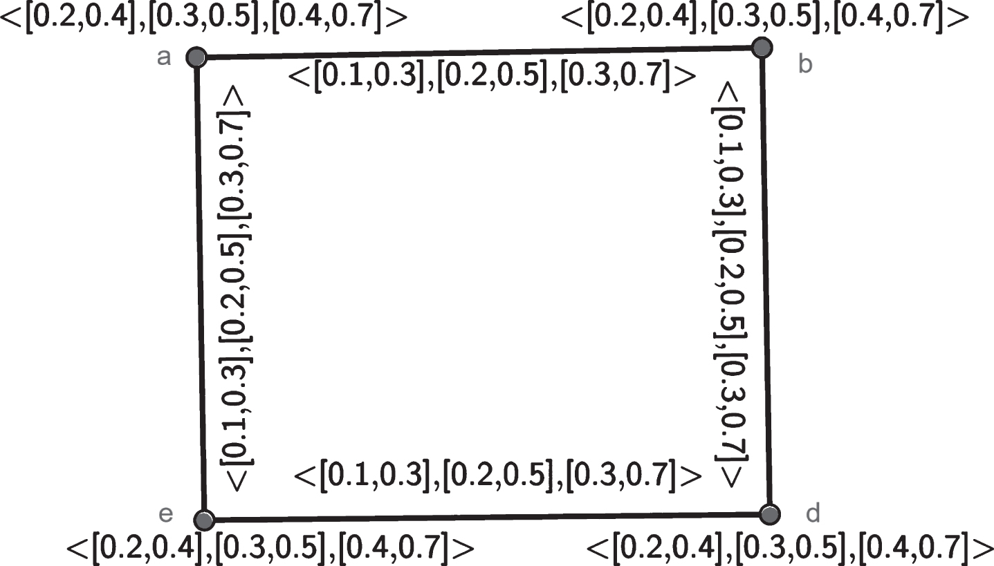
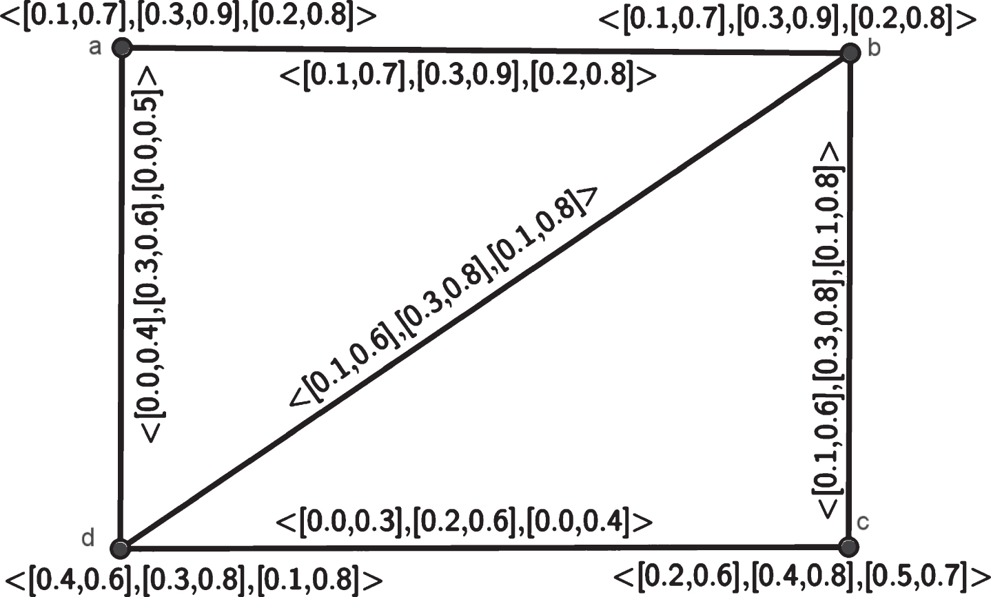
Example 3.2. Let us consider a graph G such that vertex set V = {a, b, c, d} and edge set E = {ab, bc, cd, ad}(Fig. 2). Let A be an m-PIVFS on V and B be an m-PIVFS on E defined by $\begin{matrix} A & = & (\frac{a}{< [0.2, 0.4], [0.3, 0.5], [0.4, 0.7] >}, \frac{b}{< [0.2, 0.4], [0.3, 0.5], [0.4, 0.7] >}, \\ \frac{c}{< [0.2, 0.4], [0.3, 0.5], [0.4, 0.7] >}, \frac{d}{< [0.2, 0.4], [0.3, 0.5], [0.4, 0.7] >}) . \\ B & = & (\frac{ab}{< [0.1, 0.3], [0.2, 0.5], [0.3, 0.7] >}, \frac{bc}{< [0.1, 0.3], [0.2, 0.5], [0.3, 0.7] >}, \\ \frac{cd}{< [0.1, 0.3], [0.2, 0.5], [0.3, 0.7] >}, \frac{da}{< [0.1, 0.3], [0.2, 0.5], [0.3, 0.7] >}) . \end{matrix}$

$\begin{matrix} By calculation, \deg (a) & = ([0.2, 0.6], [0.4, 1.0], [0.6, 1.4]), \\ \deg [a] & = ([0.4, 1.0], [0.7, 1.5], [1.0, 2.1]), \\ \deg (b) & = ([0.2, 0.6], [0.4, 1.0], [0.6, 1.4]), \\ \deg [b] & = ([0.4, 1.0], [0.7, 1.5], [1.0, 2.1]), \end{matrix}$

$\begin{matrix} \deg (c) & = & ([0.2, 0.6], [0.4, 1.0], [0.6, 1.4]), \\ \deg [c] & = & ([0.4, 1.0], [0.7, 1.5], [1.0, 2.1]), \\ \deg (d) & = & ([0.2, 0.6], [0.4, 1.0], [0.6, 1.4]), \\ \deg [d] & = & ([0.4, 1.0], [0.7, 1.5], [1.0, 2.1]) . \end{matrix}$

Fig. 2

Closed neighborhood degree of a 3-PIVFG G.

Thus, G is a regular m-PIVFG as well as totally regular m-PIVFG.

Definition 3.5. An m-PIVFG G = (V, A, B) of G^* = (V, E) is said to be complete if $p_{i} \circ μ_{B}^{l} (xy) = min {p_{i} \circ μ_{A}^{l} (x), p_{i} \circ μ_{A}^{l} (y)}$ and $p_{i} \circ μ_{B}^{u} (xy) = min {p_{i} \circ μ_{A}^{u} (x), p_{i} \circ μ_{A}^{u} (y)}$ , for every pair of vertices x, y ∈ V.

By definition it is obvious that every complete m-PIVFG is totally regular, but the converse is not true.

Example 3.3. From Example 3.2, as seen in Fig. 2, it is observed that G is totally regular but not complete.

Theorem 3.1. Let G = (V, A, B) be an m-PIVFG of G^* = (V, E). Then $A = < [p_{1} \circ μ_{A}^{l}, p_{1} \circ μ_{A}^{u}], [p_{2} \circ μ_{A}^{l}, p_{2} \circ μ_{A}^{u}], . . ., [p_{i} \circ μ_{A}^{l}, p_{i} \circ μ_{A}^{u}], . . ., [p_{m} \circ μ_{A}^{l}, p_{m} \circ μ_{A}^{u}] >$ , for i = 1, 2, . . . , m is a constant mapping if and only if the subsequent properties are equivalent:

G is a regular m-PIVFG.

G is a totally regular m-PIVFG.

Proof. Suppose that $A = < [p_{1} \circ μ_{A}^{l}, p_{1} \circ μ_{A}^{u}], [p_{2} \circ μ_{A}^{l}, p_{2} \circ μ_{A}^{u}], . . ., [p_{i} \circ μ_{A}^{l}, p_{i} \circ μ_{A}^{u}], . . ., [p_{m} \circ μ_{A}^{l}, p_{m} \circ μ_{A}^{u}] >$ . Let $p_{i} \circ μ_{A}^{l} (x) = g_{i}$ and $p_{i} \circ μ_{A}^{u} (x) = h_{i}$ ; for i = 1, 2, . . . , m and ∀x ∈ V.

Now, (i) ⇒ (ii)

Let us assume that G is an m-PIVFG. Let $p_{i} \circ {deg}_{μ}^{l} (x) = r_{i}$ and $p_{i} \circ {deg}_{μ}^{u} (x) = s_{i}$ ; for i = 1, 2, . . . , m and ∀x ∈ V. So, $p_{1} \circ {deg}_{μ}^{l} [x] = p_{1} \circ {deg}_{μ}^{l} (x) + p_{1} \circ μ_{A}^{l} (x) = r_{1} + g_{1}$ and $p_{1} \circ {deg}_{μ}^{u} [x] = p_{1} \circ {deg}_{μ}^{u} (x) + p_{1} \circ μ_{A}^{u} (x) = s_{1} + h_{1}$ ; ∀x ∈ V. Similarly for others. In general, $p_{i} \circ {deg}_{μ}^{l} [x] = r_{i} + g_{i}, p_{i} \circ {deg}_{μ}^{u} [x] = s_{i} + h_{i}$ , for i = 1, 2, . . . , m and ∀x ∈ V. Thus, G is a totally regular m-PIVFG.

Again, (ii) ⇒ (i)

Let us consider that G is totally regular m-PIVFG. Afterwards, $p_{i} \circ {deg}_{μ}^{l} [x] = c_{i}, p_{i} \circ {deg}_{μ}^{u} [x] = k_{i}$ ; ∀x ∈ V. Now, for i=1, $p_{1} \circ {deg}_{μ}^{l} [x] = c_{1}$ or, $p_{1} \circ {deg}_{μ}^{l} (x) + p_{1} \circ μ_{A}^{l} (x) = c_{1}$ or, $p_{1} \circ {deg}_{μ}^{l} (x) + g_{1} = c_{1}$ or, $p_{1} \circ {deg}_{μ}^{l} (x) = c_{1} - g_{1}$ . Also, $p_{1} \circ {deg}_{μ}^{u} [x] = k_{1}$ or, $p_{1} \circ {deg}_{μ}^{u} (x) + p_{1} \circ μ_{A}^{u} (x) = k_{1}$ or, $p_{1} \circ {deg}_{μ}^{u} (x) + h_{1} = k_{1}$ or, $p_{1} \circ {deg}_{μ}^{u} (x) = k_{1} - h_{1}$ . In general, $p_{i} \circ {deg}_{μ}^{l} (x) = c_{i} - g_{i}, p_{i} \circ {deg}_{μ}^{u} (x) = k_{i} - h_{i} \forall x \in V .$ Therefore, G is a regular m-PIVFG. Consequently, (i) and (ii) are equivalent.

Theorem 3.2. Let G = (V, A, B) be an m-PIVFG where G^* is a crisp graph with an odd cycle. Then, G is a regular m-PIVFG if and only if B is a constant map.

Proof. Let $B = < [p_{1} \circ μ_{B}^{l}, p_{1} \circ μ_{B}^{u}], [p_{2} \circ μ_{B}^{l}, p_{2} \circ μ_{B}^{u}], . . ., [p_{i} \circ μ_{B}^{l}, p_{i} \circ μ_{B}^{u}], . . ., [p_{m} \circ μ_{B}^{l}, p_{m} \circ μ_{B}^{u}] >$ is a constant map, for i = 1, 2, . . . , m. Let, $p_{i} \circ μ_{B}^{l} (xy) = g_{i}$ , $p_{i} \circ μ_{B}^{u} (xy) = h_{i}$ , ∀xy ∈ E. Then, $p_{i} \circ {deg}_{μ}^{l} (x) = 2 g_{i}$ , $p_{i} \circ {deg}_{μ}^{u} (x) = 2 h_{i}$ , ∀x ∈ V. Thus, G is a regular m-PIVFG. Conversely, let G be a regular m-PIVFG. Thereafter, $p_{i} \circ {deg}_{μ}^{l} (x) = r_{i}$ , $p_{i} \circ {deg}_{μ}^{u} (x) = s_{i}$ , ∀x ∈ V. Also, let e₁, e₂, . . . , e_2n+1 be the edges of G in that order. Let $p_{i} \circ μ_{B}^{l} (e_{1}) = c_{i}$ , $p_{i} \circ μ_{B}^{u} (e_{1}) = k_{i}$ . Then, $p_{i} \circ μ_{B}^{l} (e_{2}) = r_{i} - c_{i}$ , $p_{i} \circ μ_{B}^{l} (e_{3}) = r_{i} - (r_{i} - c_{i}) = c_{i}$ , $p_{i} \circ μ_{B}^{l} (e_{4}) = r_{i} - c_{i}$ , $p_{i} \circ μ_{B}^{l} (e_{5}) = r_{i} - (r_{i} - c_{i}) = c_{i}$ and so on. Therefore, $p_{i} \circ μ_{B}^{l} (e_{j}) = {\begin{matrix} c_{i} & if j is odd \\ r_{i} - c_{i} & if j is even \end{matrix}$ for i = 1, 2, . . . , m and j = 1, 2, . . . , (2n + 1). Thus $p_{i} \circ μ_{B}^{l} (e_{1}) = c_{i}$ and $p_{i} \circ μ_{B}^{l} (e_{2 n + 1}) = c_{i}$ . So, e₁ and e_2n+1 incident at a vertex v₁. Then, $p_{i} \circ {deg}_{μ}^{l} (v_{1}) = r_{i}$ or, $p_{i} \circ {deg}_{μ}^{l} (e_{1}) + p_{i} \circ {deg}_{μ}^{l} (e_{2 n + 1}) = r_{i}$ or, c_i + c_i = r_i or, c_i = r_i/2. This proves that $p_{i} \circ μ_{B}^{l} (xy)$ is a regular function.

Similarly, $p_{i} \circ μ_{B}^{u} (e_{2}) = s_{i} - k_{i}$ , $p_{i} \circ μ_{B}^{u} (e_{3}) = s_{i} - (s_{i} - k_{i}) = k_{i}$ , $p_{i} \circ μ_{B}^{u} (e_{4}) = s_{i} - k_{i}$ , $p_{i} \circ μ_{B}^{u} (e_{5}) = s_{i} - (s_{i} - k_{i}) = k_{i}$ and so on. Therefore, $p_{i} \circ μ_{B}^{u} (e_{j}) = {\begin{matrix} k_{i} & if j is odd \\ s_{i} - k_{i} & if j is even \end{matrix}$ for i = 1, 2, . . . , m and j = 1, 2, . . . , (2n + 1). Thus $p_{i} \circ μ_{B}^{u} (e_{1}) = k_{i}$ and $p_{i} \circ μ_{B}^{u} (e_{2 n + 1}) = k_{i}$ . So, e₁ and e_2n+1 incident at a vertex v₁. Now, $p_{i} \circ {deg}_{μ}^{u} (v_{1}) = s_{i}$ or, $p_{i} \circ {deg}_{μ}^{u} (e_{1}) + p_{i} \circ {deg}_{μ}^{u} (e_{2 n + 1}) = s_{i}$ or, k_i + k_i = s_i Thus, c_i = r_i/2. This proves that $p_{i} \circ μ_{B}^{u} (xy)$ is a regular function ∀xy ∈ E. Therefore, B is a constant map.

Corollary 1. Let G be an m-PIVFG, where G^* is a usual graph having even cycle. Thereafter, G is a regular m-PIVFG if and only if $B = < [p_{1} \circ μ_{B}^{l}, p_{1} \circ μ_{B}^{u}], [p_{2} \circ μ_{B}^{l}, p_{2} \circ μ_{B}^{u}], . . ., [p_{i} \circ μ_{B}^{l}, p_{i} \circ μ_{B}^{u}], . . ., [p_{m} \circ μ_{B}^{l}, p_{m} \circ μ_{B}^{u}] >$ for i = 1, 2, . . . , m is a constant map or alternate edges have the same membership degrees.

Definition 3.6. The density of an m-PIVFG G = (V, A, B) is D (G) = ([p₁ ∘ D^l (G) , p₁ ∘ D^u (G)] , [p₂ ∘ D^l (G) , p₂ ∘ D^u (G)] , . . . , [p_i ∘ D^l (G) , p_i ∘ D^u (G)] , . . . , [p_m ∘ D^l (G) , p_m ∘ D^u (G)]); where $p_{i} \circ D^{l} (G) = \frac{2 \sum_{xy \in E} p_{i} \circ μ_{B}^{l} (xy)}{\sum_{x, y \in V} \min {p_{i} \circ μ_{A}^{l} (x), p_{i} \circ μ_{A}^{l} (y)}}$ $p_{i} \circ D^{u} (G) = \frac{2 \sum_{xy \in E} p_{i} \circ μ_{B}^{u} (xy)}{\sum_{x, y \in V} \min {p_{i} \circ μ_{A}^{u} (x), p_{i} \circ μ_{A}^{u} (y)}}$ for x, y ∈ V, provided D^l (G) < D^u (G). If the condition is not true then we have to define the density by other way.

Definition 3.7. An m-PIVFG G is balanced if D (H) ≤ D (G) i.e, p_i ∘ D^l (H) ≤ p_i ∘ D^l (G) and p_i ∘ D^u (H) ≤ p_i ∘ D^u (G) for all subgraphs H of G.

Definition 3.8. An m-PIVFG G is strictly balanced if for every x, y ∈ V, D (H) = D (G) for all non-empty subgraphs.

Theorem 3.3. Every complete m-PIVFG is balanced.

Proof. Let G = (V, A, B) be a complete m-PIVFG. Thereafter, $p_{i} \circ μ_{B}^{l} (xy) = min {p_{i} \circ μ_{A}^{l} (x), p_{i} \circ μ_{A}^{l} (y)}$ and $p_{i} \circ μ_{B}^{u} (xy) = min {p_{i} \circ μ_{A}^{u} (x), p_{i} \circ μ_{A}^{u} (y)}$ for every pair of vertices x, y ∈ V and ∀ i. Consequently, $\sum_{xy \in E} p_{i} \circ μ_{B}^{l} (xy) = \sum_{x, y \in V} \min {p_{i} \circ μ_{A}^{l} (x), p_{i} \circ μ_{A}^{l} (y)}$ and $\sum_{xy \in E} p_{i} \circ μ_{B}^{u} (xy) = \sum_{x, y \in V} \min {p_{i} \circ μ_{A}^{u} (x), p_{i} \circ μ_{A}^{u} (y)}$ . $p_{i} \circ D^{l} (G) = \frac{2 \sum_{xy \in E} p_{i} \circ μ_{B}^{l} (xy)}{\sum_{x, y \in V} \min {p_{i} \circ μ_{A}^{l} (x), p_{i} \circ μ_{A}^{l} (y)}} = \frac{2 \sum_{x, y \in V} \min {p_{i} \circ μ_{A}^{l} (x), p_{i} \circ μ_{A}^{l} (y)}}{\sum_{x, y \in V} \min {p_{i} \circ μ_{A}^{l} (x), p_{i} \circ μ_{A}^{l} (y)}} = 2 .$

Similarly we get, p_i ∘ D^u (G) =2, ∀ i. Also, every subgraph of a complete m-PIVFG is complete. Hence, it can be easily checked that D (H) = ([2, 2] , [2, 2] , . . . , [2, 2]) for m pole and for every H ⊆ G. Thus G is balanced m-PIVFG.

Note 1. Converse of above theorem is not true, that is every balanced m-PIVFG is not necessary complete.

Note 2. Let G be a self-complementary m-PIVFG. Then, D [G] = ([1, 1] , [1, 1] , . . . , [1, 1]).

Theorem 3.4. Let G be strictly balanced m-PIVFG and $\bar{G}$ be its complement; thereafter, $D (G) + D (\bar{G}) = ([2, 2], [2, 2], \dots, [2, 2])$ .

Proof. Let G be a strictly balanced m-PIVFG and $\bar{G}$ be the complement. Let H be any non-empty sub graph of G. Since, G is a strictly balanced m-PIVFG then D (G) = D (H) for any H ⊆ G and x, y ∈ V. In $\bar{G}$ ,

$p_{i} \circ μ_{\bar{B}}^{l} (xy) = \min {p_{i} \circ μ_{A}^{l} (x), p_{i} \circ μ_{A}^{l} (y)} - p_{i} \circ μ_{B}^{l} (xy)$

$p_{i} \circ μ_{\bar{B}}^{u} (xy) = \min {p_{i} \circ μ_{A}^{u} (x), p_{i} \circ μ_{A}^{u} (y)} - p_{i} \circ μ_{B}^{u} (xy)$ , for every x, y ∈ V and ∀ i.

Dividing both sides of (i) by

\min {p_{i} \circ μ_{A}^{l} (x), p_{i} \circ μ_{A}^{l} (y)}

we get,

$\frac{p_{i} \circ μ_{\bar{B}}^{l} (xy)}{\min {p_{i} \circ μ_{A}^{l} (x), p_{i} \circ μ_{A}^{l} (y)}} = 1 - \frac{p_{i} \circ μ_{B}^{l} (xy)}{\min {p_{i} \circ μ_{A}^{l} (x), p_{i} \circ μ_{A}^{l} (y)}} .$ Taking summation both sides,

$\sum \frac{p_{i} \circ μ_{\bar{B}}^{l} (xy)}{\min {p_{i} \circ μ_{A}^{l} (x), p_{i} \circ μ_{A}^{l} (y)}} = 1 - \sum \frac{p_{i} \circ μ_{B}^{l} (xy)}{\min {p_{i} \circ μ_{A}^{l} (x), p_{i} \circ μ_{A}^{l} (y)}},$ for every x, y ∈ V. Multiplying by 2 both sides, $2 \sum \frac{p_{i} \circ μ_{\bar{B}}^{l} (xy)}{\min {p_{i} \circ μ_{A}^{l} (x), p_{i} \circ μ_{A}^{l} (y)}} = 2 - 2 \sum \frac{p_{i} \circ μ_{B}^{l} (xy)}{\min {p_{i} \circ μ_{A}^{l} (x), p_{i} \circ μ_{A}^{l} (y)}}$

i.e, $p_{i} \circ D_{i}^{l} (\bar{G}) = 2 - p_{i} \circ D_{i}^{l} (G)$ . Similarly, $p_{i} \circ D^{u} (\bar{G}) = 2 - p_{i} \circ D^{u} (G)$ . Again, $D (G) + D (\bar{G}) = ([p_{1} \circ D^{l} (G), p_{1} \circ D^{u} (G)], [p_{2} \circ D^{l} (G), p_{2} \circ D^{u} (G)], \dots, [p_{m} \circ D^{l} (G), p_{m} \circ D^{u} (G)]) + ([p_{1} \circ D^{l} (\bar{G}), p_{1} \circ D^{u} (\bar{G})], [p_{2} \circ D^{l} (\bar{G}), p_{2} \circ D^{u} (\bar{G})], . . ., [p_{m} \circ D^{l} (\bar{G}), p_{m} \circ D^{u} (\bar{G})]) = ([p_{1} \circ D^{l} (G) + p_{1} \circ D^{l} (\bar{G}), p_{1} \circ D^{u} (G) + p_{1} \circ D^{u} (\bar{G})], [p_{2} \circ D^{l} (G) + p_{2} \circ D^{l} (\bar{G}), p_{2} \circ D^{u} (G) + p_{2} \circ D^{u} (\bar{G})], . . ., [p_{m} \circ D^{l} (G) + p_{m} \circ D^{l} (\bar{G}), p_{m} \circ D^{u} (G) + p_{m} \circ D^{u} (\bar{G})]) = ([2, 2], [2, 2], \dots, [2, 2])$ . This completes the proof.

Note 3. The complement of a strictly balanced m-PIVFG is also strictly balanced.

Note 4. Let G₁ and G₂ be isomorphic m-PIVFG. If G₂ is balanced then G₁ is also balanced.

4 Irregularity in m-PIVFG

In this present section, first, the irregularity in m-PIVFG with suitable examples are defined and some theorems related to that are described.

Definition 4.1. Let G = (V, A, B) be an m-PIVFG on G^* = (V, E). If there exists a vertex in G which is adjacent to vertices with distinct neighborhood degree, then G is called an irregular m-PIVFG.

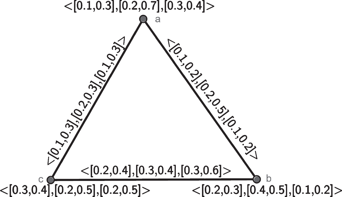
Example 4.1. Let us assume an m-PIVFG G = (V, A, B) (Fig. 3), where $\begin{matrix} A & = & (\frac{a}{< [0.1, 0.3], [0.2, 0.7], [0.3, 0.4] >}, \\ \frac{b}{[0.3, 0.4], [0.2, 0.5], [0.2, 0.5]}, \\ \frac{c}{[0.2, 0.3], [0.4, 0.5], [0.1, 0.2]}) \\ B & = & (\frac{ab}{< [0.1, 0.2], [0.2, 0.5], [0.1, 0.2] >}, \\ \frac{bc}{< [0.2, 0.4], [0.3, 0.4], [0.3, 0.6] >}, \\ \frac{ca}{< [0.1, 0.3], [0.2, 0.3], [0.1, 0.3] >}) \end{matrix}$

Fig. 3

An irregular 3-PIVFG G.

Here, deg (a) = ([0.2, 0.5] , [0.4, 0.8] , [0.2, 0.5]),

deg (b) = ([0.3, 0.6] , [0.5, 0.9] , [0.4, 0.8]),

deg (c) = ([0.3, 0.7] , [0.5, 0.7] , [0.4, 0.9]).

Thus, deg (a) ≠ deg (b) and deg (a) ≠ deg (c). Therefore, G is an irregular graph.

Definition 4.2. Let G be an m-PIVFG of a crisp graph G^*. If there exits a vertex in G which is adjacent to vertices with distinct closed neighborhood degree, then, it is said to be a totally irregular m-PIVFG.

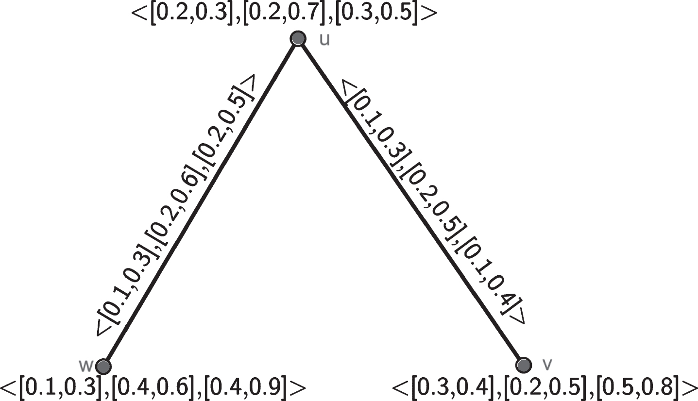
Example 4.2. Let us think about an m-PIVFG G = (V, A, B) (Fig. 4), where $\begin{matrix} A & = & (\frac{u}{< [0.1, 0.3], [0.2, 0.7], [0.3, 0.4] >}, \\ \frac{v}{[0.3, 0.4], [0.2, 0.5], [0.2, 0.5]}, \\ \frac{w}{[0.2, 0.3], [0.4, 0.5], [0.1, 0.2]}) \\ B & = & (\frac{uv}{< [0.1, 0.2], [0.2, 0.6], [0.3, 0.5] >}, \\ \frac{uw}{< [0.2, 0.3], [0.1, 0.4], [0.3, 0.4] >}) . \end{matrix}$ Here, deg [u] = ([0.4, 0.9] , [0.6, 1.8] , [0.6, 1.4]),

deg [v] = ([0.4, 0.7] , [0.4, 1.0] , [0.6, 1.2]),

deg [w] = ([0.2, 0.6] , [0.6, 1.2] , [0.6, 1.4]).

Fig. 4

A 3-PIVFG G which is totally irregular.

Hence, there exists a vertex u which has distinct closed neighbourhood degrees with the vertices v and w. Therefore, the graph shown in Fig. 4 is a totally irregular m-PIVFG.

Definition 4.3. A connected m-PIVFG G = (V, A, B) is called a neighborly irregular m-PIVFG if every two adjacent vertices of G have distinct open neighborhood values in G.

Example 4.3. Let us think about an m-PIVFG G = (V, A, B), where

$A = (\frac{u}{< [0.2, 0.3], [0.5, 0.7], [0.1, 0.4] >}, \frac{v}{< [0.1, 0.5], [0.4, 0.6], [0.2, 0.7] >}, \frac{w}{[0.2, 0.3], [0.4, 0.5], [0.1, 0.2]}, \frac{x}{< [0.1, 0.5], [0.4, 0.6], [0.2, 0.7] >})$

$B = (\frac{uv}{< [0.1, 0.3], [0.4, 0.6], [0.1, 0.4] >}, \frac{vw}{< [0.1, 0.2], [0.3, 0.6], [0.1, 0.3] >}, \frac{wx}{< [0.1, 0.3], [0.2, 0.5], [0.1, 0.2] >}, \frac{xu}{< [0.1, 0.3], [0.4, 0.5], [0.1, 0.2] >})$

Here, deg (u) = ([0.2, 0.5] , [0.4, 1.0] , [0.3, 0.7]),

deg (v) = ([0.2, 0.5] , [0.4, 1.2] , [0.3, 0.7]),

deg (w) = ([0.2, 0.5] , [0.7, 1.0] , [0.2, 0.7]),

deg (x) = ([0.2, 0.5] , [0.6, 0.8] , [0.2, 0.7]).

Thus, G is neighborly irregular.

Definition 4.4. A connected m-PIVFG G = (V, A, B) is said to be a neighborly totally irregular m-PIVFG if every two adjacent vertices of G have distinct closed neighborhood degree.

Example 4.4. From Fig. 5, we get,

Fig. 5

A 3-PIVFG G which is neighborly irregular.

deg [u] = ([0.4, 0.8] , [0.9, 1.7] , [0.4, 1.1]),

deg [w] = ([0.4, 0.8] , [1.2, 1.7] , [0.3, 1.1]),

deg [v] = ([0.3, 1.0] , [0.8, 1.8] , [0.5, 1.4]),

deg [x] = ([0.3, 1.0] , [1.0, 1.4] , [0.4, 1.4]) .

Since, every two adjacent vertices of G having different closed neighborhood grades G is neighborly totally irregular m-PIVFG.

Definition 4.5. Let G be connected m-PIVFG. G is said to be a highly irregular m-PIVFG if every vertex of G is adjacent to vertices in G with distinct neighborhood values.

Example 4.5. It is clearly observed that G of example 4.3 is highly irregular.

Theorem 4.1. An m-PIVFG G is highly neighborly irregular m-PIVFG iff neighborhood degrees of all vertices of G are different.

Proof. Let an m-PIVFG G is highly irregular as well as neighborly irregular m-PIVFG. Also let $\deg (v_{j}) = ([s_{j}^{1}, t_{j}^{1}], [s_{j}^{2}, t_{j}^{2}], \dots, [s_{j}^{m}, t_{j}^{m}])$ and adjacent vertices of v₁ be v₂, v₃, ⋯ v_n with neighborhood degrees $([s_{2}^{1}, t_{2}^{1}], [s_{2}^{2}, t_{2}^{2}], \dots, [s_{2}^{m}, t_{2}^{m}])$ , $([s_{3}^{1}, t_{3}^{1}], [s_{3}^{2}, t_{3}^{2}], \dots, [s_{3}^{m}, t_{3}^{m}])$ ,⋯, $([s_{n}^{1}, t_{n}^{1}], [s_{n}^{2}, t_{n}^{2}], \dots, [s_{n}^{m}, t_{n}^{m}])$ respectively. Then, since G is highly irregular, $s_{2}^{i} \neq s_{3}^{j} \neq \dots \neq s_{n}^{j}$ and $t_{2}^{i} \neq t_{3}^{j} \neq \dots \neq t_{n}^{j}$ . Again since G is neighborly irregular, then $s_{1}^{j} \neq s_{2}^{i} \neq s_{3}^{j} \neq \dots \neq s_{n}^{j}$ and $t_{1}^{j} \neq t_{2}^{i} \neq t_{3}^{j} \neq \dots \neq t_{n}^{j}$ , for each i = 1, 2, ⋯ , m. Therefore, the neighborhood grades of all the vertices of G are different.

Conversely, let the neighborhood grades of all the vertices of G are different, then $s_{1}^{j} \neq s_{2}^{i} \neq s_{3}^{j} \neq \dots \neq s_{n}^{j}$ and $t_{1}^{j} \neq t_{2}^{i} \neq t_{3}^{j} \neq \dots \neq t_{n}^{j}$ . So, G is highly irregular as well as neighborly irregular.

Theorem 4.2. An m-PIVFG G = (V, A, B) of some crisp graph G^* = (V, E) with a cycle of 3 vertices is highly irregular as well as neighborly irregular m-PIVFG iff for each pole of the vertices both the membership values upper and lower between every pair of vertices are all distinct.

Proof. Let us consider that for each pole of the vertices both the membership values lower and upper are all different.

Case I:

Let x, y, z ∈ V.

Given that, $p_{i} \circ μ_{A}^{l} (x) \neq p_{i} \circ μ_{A}^{l} (y) \neq p_{i} \circ μ_{A}^{l} (z)$ and $p_{i} \circ μ_{A}^{u} (x) \neq p_{i} \circ μ_{A}^{u} (y) \neq p_{i} \circ μ_{A}^{u} (z)$ , for each i = 1, 2, ⋯ , m. Then, $\sum_{x \in N (x)} p_{i} \circ μ_{A}^{l} (x) \neq \sum_{x \in N (x)} p_{i} \circ μ_{A}^{l} (y) \neq \sum_{x \in N (x)} p_{i} \circ μ_{A}^{l} (z)$ , i.e., $p_{i} \circ {deg}_{μ}^{l} (x) \neq p_{i} \circ {deg}_{μ}^{l} (y) \neq p_{i} \circ {deg}_{μ}^{l} (z)$ . Similarly $p_{i} \circ {deg}_{μ}^{u} (x) \neq p_{i} \circ {deg}_{μ}^{u} (y) \neq p_{i} \circ {deg}_{μ}^{u} (z)$ . Hence, G is neighborly irregular and highly irregular.

Case II:

Let G be highly irregular and neighborly irregular. Let deg (x) = (p₁ ∘ deg(x) , p_i ∘ deg(x) , ⋯ , p_i ∘ deg(x)) = ([s¹, t¹] , [s², t²] , ⋯ , [s^m, t^m]). Now let us assume both the membership values lower and upper of any two distinct vertices are same for each pole. Let x, y ∈ V. Let $p_{i} \circ μ_{A}^{l} (x) = p_{i} \circ μ_{A}^{l} (y)$ and $p_{i} \circ μ_{A}^{u} (x) = p_{i} \circ μ_{A}^{u} (y)$ , for i = 1, 2, ⋯ , m. Then, deg (x) = deg (y). Since G^* is cyclic, it contradicts the idea that G is a neighborly irregular as well as highly irregular m-PIVFG. Hence our assumption is wrong. Hence for each pole, the lower and upper membership values of all the vertices of G are all different.

Note 5. A neighborly irregular m-PIVFG may not be neighborly total irregular.

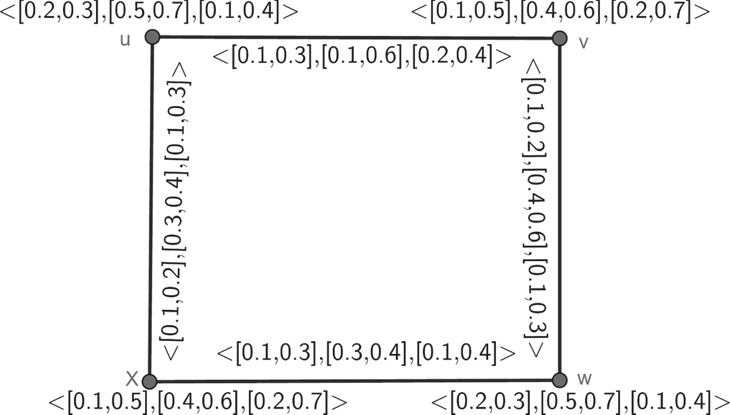
Example 4.6. Let us consider an m-PIVFG G = (V, A, B) (Fig. 6), where $\begin{matrix} A & = & (\frac{a}{< [0.2, 0.5], [0.7, 0.8], [0.2, 0.3] >}, \\ \frac{b}{[0.1, 0.4], [0.6, 0.7], [0.4, 0.9]}, \\ \frac{c}{[0.1, 0.3], [0.5, 1.0], [0.4, 0.6]}, \\ \frac{d}{< [0.1, 0.2], [0.2, 0.3], [0.4, 0.8] >}, \\ \frac{e}{< [0.2, 0.4], [0.6, 0.7], [0.3, 0.9] >}) \\ B & = & (\frac{ab}{< [0.1, 0.3], [0.2, 0.6], [0.1, 0.3] >}, \\ \frac{bc}{< [0.0, 0.1], [0.3, 0.5], [0.2, 0.6] >}, \\ \frac{cd}{< [0.1, 0.2], [0.3, 0.3], [0.1, 0.6] >}, \\ \frac{da}{< [0.0, 0.1], [0.2, 0.3], [0.1, 0.3] >}, \\ \frac{de}{< [0.1, 0.2], [0.1, 0.3], [0.2, 0.7] >}) . \end{matrix}$

Fig. 6

Neighborly irregular but not neighborly total irregular 3-PIVFG G.

Here, deg (a) = ([0.1, 0.4] , [0.4, 0.9] , [0.2, 0.6]) ,

deg [a] = ([0.3, 0.9] , [1.1, 1.7] , [0.4, 0.9]),

deg (b) = ([0.1, 0.4] , [0.5, 1.1] , [0.3, 0.9]) ,

deg [b] = ([0.2, 0.6] , [1.1, 1.8] , [0.7, 1.8]),

deg (c) = ([0.1, 0.3] , [0.6, 0.8] , [0.3, 1.2]) ,

deg [c] = ([0.2, 0.6] , [1.1, 1.8] , [0.7, 1.8]),

deg (d) = ([0.2, 0.5] , [0.6, 0.9] , [0.4, 1.6]) ,

deg [d] = ([0.3, 0.7] , [0.8, 1.2] , [0.8, 2.4]),

deg (e) = ([0.1, 0.2] , [0.1, 0.3] , [0.2, 0.7]) ,

deg [e] = ([0.1, 0.3] , [0.5, 1.0] , [0.5, 1.6]) .

Here, deg (b)= deg (c) but deg [b]=deg [c]. That means two adjacent vertices b and c have same closed neighborhood degree. Thus, G is neighborly irregular but not neighborly total irregular.

Theorem 4.3. If an m-PIVFG G is neighborly irregular m-PIVFG and $([p_{1} \circ μ_{A}^{l}, p_{1} \circ μ_{A}^{u}], [p_{2} \circ μ_{A}^{l}, p_{2} \circ μ_{A}^{u}], \dots, [p_{m} \circ μ_{A}^{l}, p_{m} \circ μ_{A}^{u}])$ is a constant map, then it is neighborly totally irregular m-PIVFG.

Proof. Let G be a neighborly irregular m-PIVFG. Then, the open neighborhood degrees of every two adjacent vertices are distinct. Let x, y ∈ V be adjacent vertices with distinct open neighborhood degrees, i.e., deg (x) = ([s₁, t₁] , [s₂, t₂] , ⋯ , [s_m, t_m]) and deg (y) = ([k₁, l₁] , [k₂, l₂] , ⋯ , [k_m, l_m]), where s + i ≠ t_i and k_i ≠ l_i. Let p_i ∘ μ^l (x) = c₁ and p_i ∘ μ^u (x) = c₂. Since $[p_{i} \circ μ_{A}^{l}, p_{i} \circ μ_{A}^{u}]$ is constant function, $p_{i} \circ {deg}_{μ}^{l} [x] = p_{i} \circ {deg}_{μ}^{l} (x) + p_{i} \circ μ^{l} (x) = s_{i} + c_{1}$ and $p_{i} \circ {deg}_{μ}^{u} [x] = p_{i} \circ {deg}_{μ}^{u} (x) + p_{i} \circ μ^{u} (x) = t_{i} + c_{2}$ . Similarly, $p_{i} \circ deg μ^{l} [y] = p_{i} \circ {deg}_{μ}^{l} (y) + p_{i} \circ μ^{l} (y) = k_{i} + c_{1}$ and $p_{i} \circ {deg}_{μ}^{u} [y] = p_{i} \circ {deg}_{μ}^{u} (y) + p_{i} \circ μ^{u} (y) = l_{i} + c_{2}$ . Now let us claim that $p_{i} \circ {deg}_{μ}^{l} [x] = p_{i} \circ {deg}_{μ}^{l} [y]$ and $p_{i} \circ {deg}_{μ}^{u} [x] = p_{i} \circ {deg}_{μ}^{u} [y]$ . Consider $p_{i} \circ {deg}_{μ}^{l} [x] = p_{i} \circ {deg}_{μ}^{l} [y]$ or, s_i + c₁ = k_i + c₁ or, s_i = k_i, for all i = 1, 2, ⋯ , m. This contradicts the fact that s_i ≠ k_i or $p_{i} \circ {deg}_{μ}^{l} [x] \neq p_{i} \circ {deg}_{μ}^{l} [y]$ . Similarly for $p_{i} \circ {deg}_{μ}^{u} [x] = p_{i} \circ {deg}_{μ}^{u} [y]$ or, t_i + c₂ = l_i + c₂ or, t_i = l_i, for all i = 1, 2, ⋯ , m. Which contradicts the fact that t_i ≠ l_i or, $p_{i} \circ {deg}_{μ}^{u} [x] \neq p_{i} \circ {deg}_{μ}^{u} [y]$ . Thus, G is a highly totally irregular m-PIVFG.

5 Free node and busy node

In this section, some definitions of free nodes and busy nodes of m-PIVFG are defined and demonstrated with the help of suitable examples. Some theorems related to these are proposed.

Definition 5.1. A node x of an m-PIVFG is called l-busy node if $p_{i} \circ μ^{l} (x) \leq p_{i} \circ \deg_{μ}^{l} (x)$ , ∀i otherwise the node x is said to be l-free node.

Similarly, a node x of an m-PIVFG is said to be u-busy node if $p_{i} \circ μ^{u} (x) \leq p_{i} \circ \deg_{μ}^{u} (x)$ , ∀i otherwise the node x is called u-free node.

Definition 5.2. A node x of an m-PIVFG G = (V, A, B) is said to be

l-partial free node if it is l-free node in both G and $\bar{G}$ .

l-fully free node if it l-free node in G but it is a l-busy node in $\bar{G}$ .

l-partial busy node if it is a l-busy node in both G and $\bar{G}$ .

l-fully busy node if it l-busy node in G but it is a l-free node in $\bar{G}$ .

Definition 5.3. A node x of an m-PIVFG G = (V, A, B) is said to be

u-partial free node if it is u-free node in both G and $\bar{G}$ .

u-fully free node if it u-free node in G but it is a u-busy node in $\bar{G}$ .

u-partial busy node if it is a u-busy node in both G and $\bar{G}$ .

u-fully busy node if it u-busy node in G but it is a u-free node in $\bar{G}$ .

Example 5.1. Let us consider an m-PIVFG (Fig. 7) where, $A = (\frac{a}{< [0.1, 0.7], [0.3, 0.9], [0.2, 0.8] >}, \frac{b}{[0.1, 0.7], [0.3, 0.9], [0.2, 0.8]}, \frac{c}{[0.2, 0.6], [0.4, 0.8], [0.5, 0.7]}, \frac{d}{< [0.4, 0.6], [0.3, 0.8], [0.1, 0.8] >})$ .

$B = (\frac{ad}{< [0.1, 0.2], [0.0, 0.2], [0.1, 0.3] >}, \frac{ac}{< [0.1, 0.6], [0.3, 0.8], [0.2, 0.7] >}, \frac{dc}{< [0.2, 0.3], [0.1, 0.2], [0.1, 0.3] >}, \frac{bc}{< [0.1, 0.4], [0.0, 0.5], [0.0, 0.4] >})$ .

Fig. 7

A 3-PIVFG G.

Then complement of G is depicted in Fig. 8:

Fig. 8

Complement $\bar{G}$ of a 3-PIVFG G.

$\begin{matrix} p_{1} \circ μ^{l} (a) = 0.1 = p_{1} \circ μ^{l} (\bar{a}), p_{1} \circ μ^{u} (a) = 0.7 = p_{1} \circ μ^{u} (\bar{a}), \\ p_{2} \circ μ^{l} (a) = 0.3 = p_{2} \circ μ^{l} (\bar{a}), p_{2} \circ μ^{u} (a) = 0.9 = p_{2} \circ μ^{u} (\bar{a}), \\ p_{3} \circ μ^{l} (a) = 0.2 = p_{3} \circ μ^{l} (\bar{a}), p_{3} \circ μ^{u} (a) = 0.8 = p_{3} \circ μ^{u} (\bar{a},) \end{matrix}$ Therefore, $\begin{matrix} \deg_{μ}^{l} (a) = (0.1 + 0.4, 0.3 + 0.3, 0.2 + 0.1) = (0.5, 0.6, 0.3) . \\ \deg_{μ}^{l} (\bar{a}) = (0.1 + 0.4, 0.3 + 0.3, 0.2 + 0.1) = (0.5, 0.6, 0.3) . \\ \deg_{μ}^{u} (a) = (0.6 + 0.7, 0.8 + 0.9, 0.8 + 0.8) = (1.3, 1.7, 1.6) . \\ \deg_{μ}^{u} (\bar{a}) = (0.6 + 0.7, 0.8 + 0.9, 0.8 + 0.8) = (1.3, 1.7, 1.6) . \end{matrix}$ Where, $\bar{a}, \bar{b}, \bar{c}, \bar{d}$ represents vertices of $\bar{G}$ . Hence, node a is l-busy node in both G and $\bar{G}$ . Thus, a is l-partial busy node. And, also node a is u-busy node in both G and $\bar{G}$ . Thus a is u-partial busy node. Similarly, $\begin{matrix} p_{1} \circ μ^{l} (b) = 0.1 = p_{1} \circ μ^{l} (\bar{b}), p_{1} \circ μ^{u} (b) = 0.7 = p_{1} \circ μ^{u} (\bar{b}), \\ p_{2} \circ μ^{l} (b) = 0.3 = p_{2} \circ μ^{l} (\bar{b}), p_{2} \circ μ^{u} (b) = 0.9 = p_{2} \circ μ^{u} (\bar{b}), \\ p_{3} \circ μ^{l} (b) = 0.2 = p_{3} \circ μ^{l} (\bar{b}), p_{3} \circ μ^{u} (b) = 0.8 = p_{3} \circ μ^{u} (\bar{b}) . \end{matrix}$ Therefore, $\begin{matrix} \deg_{μ}^{l} (b) = (0.4, 0.8, 1.0), \deg_{μ}^{l} (\bar{b}) = (0.2, 0.4, 0.5) . \\ \deg_{μ}^{u} (b) = (1.9, 2.2, 1.3), \deg_{μ}^{u} (\bar{b}) = (0.6, 0.8, 0.7) . \end{matrix}$

Hence, node b is l-busy node in both G and $\bar{G}$ . Thus, b is l-partial busy node. And, also node b is u-busy node in G and u-free node in $\bar{G}$ . Thus, b is u-fully busy node.

Similarly, $\begin{matrix} p_{1} \circ μ^{l} (c) = 0.2 = p_{1} \circ μ^{l} (\bar{c}), p_{1} \circ μ^{u} (c) = 0.6 = p_{1} \circ μ^{u} (\bar{c}), \\ p_{2} \circ μ^{l} (c) = 0.4 = p_{2} \circ μ^{l} (\bar{c}), p_{2} \circ μ^{u} (c) = 0.8 = p_{2} \circ μ^{u} (\bar{c}), \\ p_{3} \circ μ^{l} (c) = 0.5 = p_{3} \circ μ^{l} (\bar{c}), p_{3} \circ μ^{u} (c) = 0.7 = p_{3} \circ μ^{u} (\bar{c}) . \end{matrix}$ Therefore, $\begin{matrix} \deg_{μ}^{l} (c) = (0.5, 0.6, 0.3), \deg_{μ}^{l} (\bar{c}) = (0.6, 0.9, 0.5) . \\ \deg_{μ}^{u} (c) = (1.3, 1.7, 1.6), \deg_{μ}^{u} (\bar{c}) = (2.0, 2.6, 2.4) . \end{matrix}$

Hence, node c is l-free node in G and l-busy node in $\bar{G}$ . Thus, c is l-fully free node. And, also node c is u-busy node in both G and $\bar{G}$ . Thus, c is u-partial busy node.

Similarly, $\begin{matrix} p_{1} \circ μ^{l} (d) = 0.4 = p_{1} \circ μ^{l} (\bar{d}), p_{1} \circ μ^{u} (d) = 0.6 = p_{1} \circ μ^{u} (\bar{d}), \\ p_{2} \circ μ^{l} (d) = 0.3 = p_{2} \circ μ^{l} (\bar{d}), p_{2} \circ μ^{u} (d) = 0.8 = p_{2} \circ μ^{u} (\bar{d}), \\ p_{3} \circ μ^{l} (d) = 0.1 = p_{3} \circ μ^{l} (\bar{d}), p_{3} \circ μ^{u} (d) = 0.8 = p_{3} \circ μ^{u} (\bar{d}) . \end{matrix}$ Therefore, $\begin{matrix} \deg_{μ}^{l} (d) = (0.4, 1.0, 0.9), \deg_{μ}^{l} (\bar{d}) = (0.3, 0.7, 0.7) . \\ \deg_{μ}^{u} (d) = (2.0, 2.6, 2.3), \deg_{μ}^{u} (\bar{d}) = (1.3, 1.7, 1.5) . \end{matrix}$ Hence, the node d is l-busy in the graph G and its complement, i.e., d is l-partial busy node. Also the node d is u-busy node in the graph G and its complement. Thus, d is u-partial busy node.

Definition 5.4. An edge (x, y) of an m-PIVFG is known as an effective edge if p_i ∘ μ^l (xy) = min {p_i ∘ μ^l (x) , p_i ∘ μ^l (y)} and p_i ∘ μ^u (xy) = min {p_i ∘ μ^u (x) , p_i ∘ μ^u (y)}, ∀i = 1, 2, ⋯ m.

Theorem 5.1. If an m-PIVFG has some effective edges, then it has atleast one l-busy node and one u-busy node.

Proof. Assume that G = (V, A, B) be an m-PIVFG, has a few effective edges. Let (x, y) be an effective edge of G. Without loss of generality, we consider that p_i ∘ μ^l (x) ≤ p_i ∘ μ^l (y), ∀i. Then, clearly $p_{i} \circ {deg}_{μ}^{l} (x) \geq p_{i} \circ {deg}_{μ}^{l} (y)$ , ∀i. Therefore, l is busy node. Similarly, for p_i ∘ μ^u (x) ≤ p_i ∘ μ^u (y), ∀i i.e $p_{i} \circ {deg}_{μ}^{u} (x) \geq p_{i} \circ {deg}_{μ}^{u} (y)$ , ∀i. Hence, u is also a busy node.

Theorem 5.2. If a complete m-PIVFG has n-nodes with n > 1 then it has atleast (n - 1) l-fully busy node and nu-fully busy nodes.

Proof. Let G be an m-PIVFG with n-nodes. Also let G be complete m-PIVFG. Let us consider the nodes as x₁, x₂, x₃, ⋯ x_n such that, p_i ∘ μ^l (x₁) ≥ p_i ∘ μ^l (x₂) ≥ p_i ∘ μ^l (x₃) ≥ ⋯ ≥ p_i ∘ μ^l (x_n).

Thereafter, let for i = 1, $p_{1} \circ {deg}_{μ}^{l} (x_{1}) = p_{1} \circ μ^{l} (x_{2}) + p_{1} \circ μ^{l} (x_{3}) + \dots + p_{1} \circ μ^{l} (x_{n})$ . In general, $p_{1} \circ {deg}_{μ}^{l} (x_{k}) = (k - 1) p_{1} \circ μ^{l} (x_{k}) + p_{1} \circ μ^{l} (x_{k + 1}) + \cdot + p_{1} \circ μ^{l} (x_{n}), for k = 2, 3, \dots, (n - 1)$ , $p_{1} \circ {deg}_{μ}^{l} (x_{n}) = (n - 1) p_{1} \circ μ^{l} (x_{n}) .$ From the above equations it conclude that $p_{1} \circ {deg}_{μ}^{l} (x_{k}) > p_{1} \circ μ^{l} (x_{k}), for j = 1, 2, \dots, n$ . Also for i = 1, 2, ⋯ , m we can similarly conclude that $p_{i} \circ {deg}_{μ}^{l} (x_{k}) > p_{i} \circ μ^{l} (x_{k}), for k = 1, 2, \dots, n$ . Therefore, there exists atleast (n - 1) l-busy nodes in G. Since, G is complete m-PIVFG therefore $\bar{G}$ contains only isolated nodes, therefore it has (n - 1) l-free nodes. Hence, there exists at least (n - 1) l-fully busy nodes in a complete m-PIVFG. Again let us consider the nodes as x₁, x₂, x₃, ⋯ x_n such that, p_i ∘ μ^u (x₁) ≥ p_i ∘ μ^u (x₂) ≥ p_i ∘ μ^u (x₃) ≥ ⋯ ≥ p_i ∘ μ^u (x_n). Henceforth, let for i = 1, $p_{1} \circ {deg}_{μ}^{u} (x_{1}) = p_{1} \circ μ^{u} (x_{2}) + p_{1} \circ μ^{u} (x_{3}) + \dots + p_{1} \circ μ^{u} (x_{n})$ . In general, $p_{1} \circ {deg}_{μ}^{u} (x_{k}) = (k - 1) p_{1} \circ μ^{u} (x_{k}) + p_{1} \circ μ^{u} (x_{k + 1}) + \cdot + p_{1} \circ μ^{u} (x_{n}), for k = 2, 3, \dots, (n - 1)$ , $p_{1} \circ {deg}_{μ}^{u} (x_{n}) = (n - 1) p_{1} \circ μ^{u} (x_{n})$ . From the above equations it conclude that $p_{1} \circ {deg}_{μ}^{u} (x_{k}) \geq p_{1} \circ μ^{u} (x_{k}),$ for k = 1, 2, ⋯ , n . Also for i = 1, 2, ⋯ , m, we can similarly conclude that $p_{i} \circ {deg}_{μ}^{u} (x_{k}) \geq p_{i} \circ μ^{u} (x_{k}),$ for k = 1, 2, ⋯ , n. Therefore, there exists n u-busy nodes in G. Since, G is complete G-PIVFG therefore $\bar{G}$ contains only isolated nodes, therefore it has n u-free nodes. Hence, there exists n u-fully busy nodes in a complete m-PIVFG.

6 Application

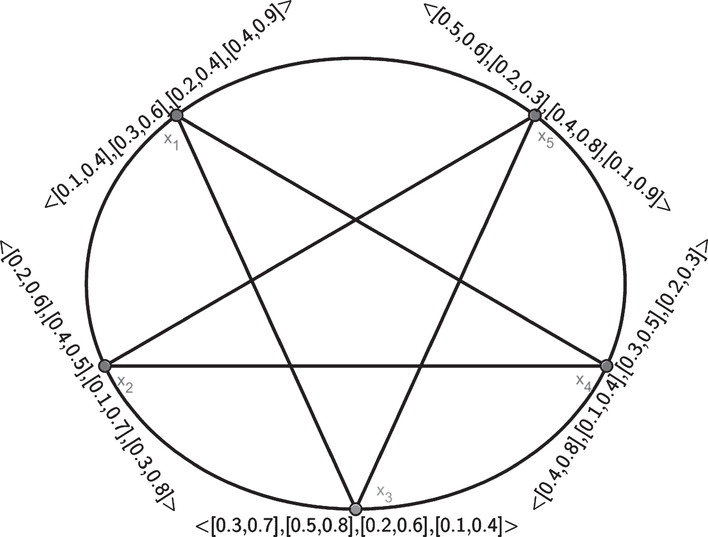
In recent days fuzzy graphs have wide range of applications in computer networks, social networks, robotics, medical diagnosis, engineering field and so on. That is, where there is a case of uncertainties that means in a decision making problem IVFG and m-PIVFG are used to simplify that type of problems. Our proposed idea m-PIVFG has more advantages than that of these two type of networks IVFGs and m-PIVFGs. This type of network allows to assign membership values in the form of an interval [0, 1]. Henceforth this types of network is used to various real life problems in multipolar decision making problems. Here we consider a case when a customer want to buy a mobile from a well-known company within a certain amount. Herein, different companies Samsung (x₁), Apple (x₂), Huawei (x₃), Oppo (x₄) and Xiaomi (x₅) are taken as different nodes. An edge is drawn between any two nodes if there is a m-polar fuzzy relation between them. The customer prefers some different features such as operating system, internal memory/RAM, camera quality, high demand/rating which are taken as pole (p_i) of every companies (Fig. 9). These features are taken as poles of every companies. Here the membership value of each pole indicates the interval of preference depending on these qualities. That means among these companies one may have top operating system, average memory, good camera quality and may be in high demand and so on within his range. Thus this is a multivalued information between any two companies which is judged in some interval in [0, 1]. This type of decision making problem is an real life example of our proposed structure of m-PIVFG.

Fig. 9

A 4-PIVFG G.

Membership value for each edge is given by Table 2.

Table 2

Membership value assigned to each pole(p_i) of each edge.

Edges	p ₁	p ₂	p ₃	p ₄
x ₁ x ₂	[0.1,0.4]	[0.3,0.5]	[0.1,0.4]	[0.3,0.8]
x ₁ x ₃	[0.1,0.4]	[0.3,0.5]	[0.1,0.4]	[0.3,0.8]
x ₁ x ₄	[0.1,0.4]	[0.3,0.5]	[0.1,0.4]	[0.3,0.8]
x ₁ x ₅	[0.1,0.4]	[0.3,0.5]	[0.1,0.4]	[0.3,0.8]
x ₂ x ₃	[0.1,0.4]	[0.3,0.5]	[0.1,0.4]	[0.3,0.8]
x ₂ x ₄	[0.1,0.4]	[0.3,0.5]	[0.1,0.4]	[0.3,0.8]
x ₂ x ₅	[0.1,0.4]	[0.3,0.5]	[0.1,0.4]	[0.3,0.8]
x ₃ x ₄	[0.1,0.4]	[0.3,0.5]	[0.1,0.4]	[0.3,0.8]
x ₃ x ₅	[0.1,0.4]	[0.3,0.5]	[0.1,0.4]	[0.3,0.8]
x ₄ x ₅	[0.1,0.4]	[0.3,0.5]	[0.1,0.4]	[0.3,0.8]

Comparing these features among all these companies we have taken a weight operator $w (x_{j}) = \frac{1 + μ_{A}^{u} (x_{j}) - μ_{A}^{l} (x_{j})}{2} \dots (1)$ for each pole p_i and for each j = 1, 2, 3, 4, 5. Thus for each pole we are calculating weight for each companies accordingly. Hence, for first pole (that means for operating system), $w (x_{1}) = \frac{1 + 0.4 - 0.1}{2} = 0.65$ , similarly w (x₂)=0.7, w (x₃)=0.7, w (x₄)=0.7, w (x₅)=0.55. Thus for second pole (that means for internal memory), w (x₁)=0.65, w (x₂)=0.55, w (x₃)=0.65, w (x₄)=0.65, w (x₅)=0.55. Thus for third pole (that means for camera quality), w (x₁)=0.6, w (x₂)=0.8, w (x₃)=0.7, w (x₄)=0.6, w (x₅)=0.7. Thus for fourth pole (that means for demand/rating), w (x₁)=0.75, w (x₂)=0.75, w (x₃)=0.65, w (x₄)=0.55, w (x₅)=0.9. Depending on these weight we calculate a ranking table (shown in Table 3).

Table 3

Rank (R_i) allotted to each company

Features	R ₁	R ₂	R ₃	R ₄	R ₅
p ₁	x₂ x₃ & x₄	x ₁	x ₅
p ₂	x₁ x₃ & x₄	x₂ & x₅
p ₃	x ₂	x₃ & x₅	x₁ & x₄
p ₄	x ₅	x₁ & x₂	x ₃	x ₄

Depending on these features, suppose r_i be the preference of feature i for rank R_i. Obviously r_i > r_j for i < j and r₁ = 5, r₂ = 4, r₃ = 3, r₄ = 2 and r₅ = 1. Thus the combined preference score is given by the formula $S_{i} = \sum_{i = 1}^{5} r_{i}$ (such as for x₁, S₁ = r₂ + r₁ + r₃ + r₂ = 4 +5 + 3 +4 = 16). Therefore, the preferences of all mobile companies are calculated in Table 4.

Table 4

Preference of all mobile

Candidate	Score
Samsung	16
Apple	18
Huawei	17
Oppo	15
Xiaomi	16

Hence, he can buy a mobile from Apple company with all these better features. It is very necessary for a person to take an appropriate decision to select a company’s mobile so that he can buy a better mobile with all these features. This type of multipolar determination is an example of decision making problem which is also suitable example of m-PIVFG.

7 Conclusion and future research direction

IVFGs and m-PFGs being viewed as generalizations of fuzzy and bi-polar fuzzy graphs respectively. In this article, we introduce m-PIVFG and its complements are illustrated through examples. We also explain the definition of neighbourhood degrees, closed neighbourhood degrees of m-PIVFG with proper examples. Also, we have stated balanced m-PIVFG, regularity in m-PIVFG and density and some properties related to regularity of m-PIVFG and balanced m-PIVFG. We also explain irregularity in m-PIVFG and some properties regarding itself. Free nodes and busy nodes in m-PIVFG are also discussed with supporting examples and theorems. In future, we shall investigate other results of m-PIVFG and extend them to solve various decision making problems under fuzzy environment.

Footnotes

Acknowledgment

The authors are cordially thankful to the Editor-in-Chief, Professor Reza Langari, the area Editor and all the anonymous reviewers for their constructive comments which led to strongly improve the quality of the paper.

References

Kaufmann

, Introduction to the theory of fuzzy subsets, 1975.

Rosenfeld

, Fuzzy graphs, in Fuzzy sets and their applications to cognitive and decision processes, (1975), pp. 77–95, Elsevier.

Zhang

W.-R.

, Bipolar fuzzy sets and relations: a computational framework for cognitive modeling and multiagent decision analysis, in NAFIPS/IFIS/NASA’94. Proceedings of the First International Joint Conference of The North American Fuzzy Information Processing Society Biannual Conference. The Industrial Fuzzy Control and Intellige, (1994), pp. 305–309, IEEE.

Zhang

W.-R.

, Bipolar fuzzy sets, in 1998 IEEE International Conference on Fuzzy Systems Proceedings. IEEE World Congress on Computational Intelligence (Cat. No. 98CH36228) 1 (1998), pp. 835–840, IEEE.

Mordeson

J.N.

and Chang-Shyh

, Operations on fuzzy graphs, Information Sciences 79(3-4) (1994), 159–170.

Mordeson

J.N.

and Nair

P.S.

, Cycles and cocycles of fuzzy graphs, Information Sciences 90(1-4) (1996), 39–49.

Mordeson

J.N.

and Nair

P.S.

, Applications of fuzzy graphs, in Fuzzy Graphs and Fuzzy Hypergraphs, (2000), pp. 83–133, Springer.

Sunitha

, Studies on fuzzy graphs, Depart of mathematics Cochin university of Science and Technology Cochin, India, 2001.

Sunitha

and Vijayakumar

, Complement of a fuzzy graph, Indian Journal of Pure and Applied Mathematics 33(9) (2002), 1451–1464.

10.

Nagoorgani

and Chandrasekaran

, Free nodes and busy nodes of a fuzzy graph, East Asian Mathematical Journal 22(2) (2006), 163–170.

11.

Shannon

and Atanassov

, On a generalization of intuitionistic fuzzy graphs, Notes on Intuitionistic Fuzzy Sets 12(1) (2006), 24–29.

12.

Nagoorgani

and Radha

, On regular fuzzy graphs, Journal of Physical Sciences 12 (2008), 33–40.

13.

Hongmei

and Lianhua

, Interval-valued fuzzy subsemi-groups and subgroups associated by interval-valued fuzzy graphs, in 2009 WRI global congress on intelligent systems 1 (2009), 484–487, IEEE.

14.

Akram

and Dudek

W.A.

, Interval-valued fuzzy graphs, Computers & Mathematics with Applications 61(2) (2011), 289–299.

15.

Rashmanlou

, Pal

, Borzooei

R.A.

, Mofidnakhaei

and Sarkar

, Product of interval-valued fuzzy graphs and degree, Journal of Intelligent & Fuzzy Systems, no. Preprint, (2018), pp. 1–9.

16.

Al-Hawary

, Complete fuzzy graphs, International J Math Combin 4 (2011), 26–34.

17.

Nagoorgani

and Malarvizhi

, Isomorphism on fuzzy graphs, International Journal of Computational and Mathematical Sciences 2(4) (2008), 190–196.

18.

Nagoorgani

and Malarvizhi

, Isomorphism properties on strong fuzzy graphs, International Journal of Algorithms, Computing and Mathematics 2(1) (2009), 39–47.

19.

Akram

, Bipolar fuzzy graphs, Information Sciences 181(24) (2011), 5548–5564.

20.

Akram

, Bipolar fuzzy graphs with applications, Knowledge-Based Systems 39 (2013), 1–8.

21.

Chen

, Li

, Ma

and Wang

, m-polar fuzzy sets: an extension of bipolar fuzzy sets, The Scientific World Journal 2014, 2014.

22.

Rashmanlou

, Samanta

, Pal

and Borzooei

, Bipolar fuzzy graphs with categorical properties, International Journal of Computational Intelligence Systems 8 (2015), 808–818.

23.

Samanta

and Pal

, Fuzzy tolerance graphs, International Journal of Latest Trends in Mathematics 1(2) (2011), 57–67.

24.

Samanta

and Pal

, Fuzzy threshold graphs, CIIT International Journal of Fuzzy Systems 3(12) (2011), 360–364.

25.

Samanta

and Pal

, Fuzzy k-competition graphs and p-competition fuzzy graphs, Fuzzy Information and Engineering 5(2) (2013), 191–204.

26.

Samanta

and Pal

, Fuzzy planar graphs, IEEE Transactions on Fuzzy Systems 23(6) (2015), 1936–1942.

27.

Talebi

and Rashmanlou

, Isomorphism on interval-valued fuzzy graphs, Annals of Fuzzy Mathematics and Informatics 6(1) (2013), 47–58.

28.

Ghorai

and Pal

, Some properties of m-polar fuzzy graphs, Pacific Science Review A: Natural Science and Engineering 18(1) (2016), 38–46.

29.

Ghorai

and Pal

, Some isomorphic properties of m-polar fuzzy graphs with applications, SpringerPlus 5(1) (2016), 2104.

30.

Ghorai

and Pal

, On some operations and density of m-polar fuzzy graphs, Pacific Science Review A: Natural Science and Engineering 17(1) (2015), 14–22.

31.

Raut

, Pal

and Ghorai

, Fuzzy permutation graph and its complements, Journal of Intelligent & Fuzzy Systems, no. Preprint, (2018), pp. 1–15.

32.

Pramanik

, Pal

, Mondal

and Samanta

, A study on bipolar fuzzy planar graph and its application in image shrinking, Journal of Intelligent & Fuzzy Systems 34(3) (2018), 1863–1874.

33.

Binu

, Mathew

and Mordeson

J.N.

, Connectivity index of a fuzzy graph and its application to human trafficking, Fuzzy Sets and Systems 360 (2019), 117–136.

34.

Jana

, Pal

and Wang

J.-Q.

, Bipolar fuzzy dombi aggregation operators and its application in multiple-attribute decision-making process, Journal of Ambient Intelligence and Humanized Computing 10(9) (2019), 3533–3549.

35.

Akram

and Sarwar

, Novel applications of m-polar fuzzy competition graphs in decision support system, Neural Computing and Applications 30(10) (2018), 3145–3165.

36.

Ghorai

and Pal

, Regular product vague graphs and product vague line graphs, Cogent Mathematics 3(1) (2016), 1213214.

37.

Ghorai

and Pal

, A note on regular bipolar fuzzy graphs neural computing and applications 21(1) (2012), 197–205, Neural Computing and Applications 30(5) (2018), 1569–1572.

38.

Ghorai

and Pal

, On degrees of m-polar fuzzy graphs with application, Journal of Uncertain Systems 11(4) (2017), 294–305.

39.

Ghorai

and Pal

, Applications of bipolar fuzzy sets in interval graphs, TWMS Journal of Applied and Engineering Mathematics 8(2) (2018), 411.

40.

Abdul-Jabbar

, Naoom

and Ouda

, Fuzzy dual graph, Journal of Al-Nahrain University 12(4) (2009), 168–171.

41.

Sahoo

and Pal

, Intuitionistic fuzzy competition graphs, Journal of Applied Mathematics and Computing 52(1-2) (2016), 37–57.

42.

Amanathulla

, Sahoo

and Pal

, L (3, 1, 1)-labeling numbers of square of paths, complete graphs and complete bipartite graphs, Journal of Intelligent & Fuzzy Systems, no. Preprint, (2019), pp. 1–9.

43.

Zadeh

L.A.

, Fuzzy sets, Information and Control 8(3) (1965), 338–353.

44.

Ghorai

and Pal

, A study on m-polar fuzzy planar graphs, International Journal of Computing Science and Mathematics 7(3) (2016), 283–292.

45.

Gorzalczany

M.B.

, A method of inference in approximate reasoning based on interval-valued fuzzy sets, Fuzzy Sets and Systems 21(1) (1987), 1–17.

46.

Bera

and Pal

, On m-polar interval-valued fuzzy graph and its application, Fuzzy Information and Engineering, 2020, https://doi.org/10.1080/16168658.2020.1785993.

47.

Mishra

and Pal

, Product of interval valued intuitionistic fuzzy graph, Annals of Pure and Applied Mathematics 5(1) (2013), 37–46.

48.

Mishra

and Pal

, Regular interval-valued intuitionistic fuzzy graphs, Journal of Informatics and Mathematical Sciences 9(3) (2017), 609–621.

49.

Pramanik

, Samanta

and Pal

, Interval-valued fuzzy planar graphs, International Journal of Machine Learning and Cybernetics 7(4) (2016), 653–664.

50.

Rashmanlou

and Pal

, Balanced interval-valued fuzzy graphs, Journal of Physical Sciences 17 (2013), 43–57.

51.

Nayeem

Sk M.A.

and Pal

, Shortest path problem on a network with imprecise edge weight, Fuzzy Optimization and Decision Making 4(4) (2005), 293–312.

52.

Rashmanlou

, Samanta

, Pal

and Borzooei

R.A.

, A study on bipolar fuzzy graphs, Journal of Intelligent & Fuzzy Systems 28(2) (2015), 571–580.