Research on the fault diagnosis method for high-speed loom using rough set and Bayesian network

Abstract

The textile industry has a long history and a large market scale around the world. High-speed loom belongs to the high-end production equipment of the textile industry with the characteristics of high precision, high speed and high efficiency. However, due to its expensive cost and complex structure, there might be significant loss once a high-speed loom breaks down. At present, the monitoring and troubleshooting of high-speed loom operation mainly depend on the experience of maintenance people to carry out inspections, which is inefficient, time-consuming, laborious and less efficient. In this paper, a fault diagnosis method for high-speed loom based on rough set and Bayesian network is investigated. Rough set theory is applied to reduce the attributes of fault causes and results and find the minimum reduction and classification rules. Then, a Bayesian fault diagnosis network model is built, and the probability of each fault cause is calculated to find the maximum probability. Finally, the diagnosis results are obtained. The experimental results have demonstrated the reliability and convenience of the faults diagnosis method for the high-speed loom.

Keywords

High-speed loom fault diagnosis rough set theory Bayesian network

1 Introduction

Fault diagnosis technology is widely used in agriculture, medical treatment, automobile and household appliances. It has also gained much research efforts in industrial applications. Especially in the textile industry, there is no mature and effective fault diagnosis system for high-speed looms because of its high cost, complex structure and various electrical equipment [1 –3]. At present, a high-speed loom is mainly based on on-site signal detection and real-time personnel monitoring. The information of high-speed looms can only be seen in factories, and the real-time data can not be saved and analyzed. When a fault happens, simple faults can be analyzed, but when the fault is complex, it can only be detected and maintained by the staff, and can not be carried out according to the operation data information. Fault analysis is far from the realization of intelligent fault diagnosis. However, with the continuous development of sensor technology, sensors can monitor the running status of high-speed looms in real-time and provide digital feedback. This investigation provides good support for fault diagnosis of high-speed looms and improves the reliability and automation of intelligent fault diagnosis system of high-speed looms.

At present, in the field of industrial fault diagnosis, support vector machine, artificial neural network and decision tree are the main diagnostic methods [4 –6]. There are many different models designed to deal with specific areas of problems, such as hydraulic systems, wind turbine systems, engine systems, etc. [7 –13] In some previous studies, Wang et al. proposed a multi-feature fusion diagnosis method of support vector machine, which extracts the typical features of fault signals, calculates the weight of each feature with information entropy, and effectively diagnoses the fault of the hydraulic system by SVM classifier [7]. A fault diagnosis method based on a multi-stage fuzzy support vector machine (FSVM) classifier for wind turbine faults is proposed by Hang et al. [8]. Empirical mode decomposition is used to extract fault eigenvectors from vibration signals, and FSVM is used to solve the problem of outlier or noise classification. Experiments show that the method has good diagnostic performance and high diagnostic accuracy. Simani et al. proposed a fault diagnosis method for wind turbine simulation model based on neural network, selected a nonlinear autoregressive network architecture with external input topology and used the high-precision quasi-base model to simulate the normal and fault behavior of wind turbine to test the fault diagnosis scheme and verify its feasibility [9]. Huang et al. proposed a fault diagnosis method combining decision tree and expert system for fuel cell engines. After data preprocessing and feature selection, they imported the training set and stored the rules in the knowledge base to get the fault results and classify the faults [10]. In the field of loom fault diagnosis, there are two kinds of fault diagnosis: fabric fault diagnosis and production system fault diagnosis. Moreover, the fault diagnosis method for high-speed loom is not mature enough. Qayum et al. used a method to find the design repetition quickly [14], applies the image processing technology to detect the textile rotary printing, and extracts the complete design pattern from the acquired image for further processing of fault detection. Seçkin and his team proposed a method about how to simulate the production process and how to use machine learning to regress from time-series data to predict the possible production failure [15], which proved to have a high success rate. Mutlu et al. put forward a method based on FMEA and FTA to analyze the ring-spinning process in the textile industry [16], so that decision-makers and engineers can easily reduce the number of hazards and risks in occupational health and safety in practice. Nazlı et al. combined the advantages of fault tree analysis (FTA) and the algorithm of fuzzy probability estimation of time (BIFPET) to improve the performance of FMEA [17], and successfully applies it to analyze and evaluate the potential risks in the finishing process of a textile company’s fabric dyeing department. GüLTEKİN proposed an image processing algorithm for the automatic detection of wear defects of yarn bobbins and fabrics [18], and achieved relatively successful results. Weldeslasie et al. discussed the diagnosis and correction of yarn faults by the expert system [19], and develops a domain knowledge model using the decision tree. Besides, the prototype system of the yarn fault knowledge base is developed and evaluated. Experiments verify the performance superiority of the prototype system.

These models and methods have some shortcomings: support vector machine is difficult to implement large-scale training samples, and it is difficult to solve multi-classification problems; the network structure of artificial neural network needs to be formulated in advance or modified by a heuristic algorithm in the training process, and excessively depends on learning samples; when dealing with inconsistent data of different types of samples by a decision tree, the information gain tends to be more numerical and easy to over-fit. Bayesian network is an uncertain causal correlation model with a strong ability to deal with uncertain problems. It can express and fuse multi-source information. However, when most attribute information of test samples is missing, the algorithm has a high false alarm rate. Rough set theory is an effective tool for dealing with ambiguity and uncertainty. It can deal with knowledge on the premise of maintaining key information and obtaining minimum knowledge representation. Chang et al. combined rough set theory and Bayesian Network to analyze the causes of influenza, and verified its effectiveness and conciseness [26]. Xie et al. put forward a fault diagnosis method combining the Bayesian network and rough set theory for the transformer system [27]. Experiments verify the feasibility and accuracy of the two methods in the field of transformer system fault diagnosis. Aiming at the blank of fault diagnosis of the high-speed loom, this paper deeply analyzes the fault types, modes and causes of the high-speed loom, and integrates rough set and Bayesian network technology into the fault diagnosis algorithm of the high-speed loom. Firstly, the fault data of high-speed loom is input into the diagnosis system, and the decision table is established by rough set theory. Then the minimum reduction table is obtained by using the reduction function of rough set attributes. Then, the Bayesian network theory is used to build the fault diagnosis model of the high-speed loom. Finally, the fault result of the high-speed loom is output. This algorithm can reduce the complexity of the diagnosis model and realize the fast and accurate analysis of the fault. The specific block diagram of the algorithm is as follows.

The rest of this paper is organized as follows: Section 2 gives an overview of rough set theory and Bayesian network theory. Section 3 enumerates the causes and results of common faults in a high-speed loom system and uses Rough set and Bayesian network theory to introduce the process of building a fault diagnosis model. Section 4 gives an example of high-speed loom fault diagnosis based on rough set and Bayesian network whose feasibility and accuracy are verified by simulation and comparing with several common fault diagnosis methods. Section 5 summarizes this work conducted in this paper.

2 Rough set theory and bayesian network

2.1 Rough set theory

Rough Set, proposed by Z. Pawlak in 1982, is a processing method for uncertain information [22]. Rough set theory is a theory for analyzing and processing data. It can deal with uncertain and incomplete data information well. It can also make full use of existing information, fully mine data, and find relevant knowledge and rules. It is core is to reduce the data, then analyze and process it, and finally get the solution [23 –25].

2.1.1 Knowledge theory of rough set

In the theory of rough set, knowledge is regarded as a kind of ability to classify objects. Their attribute sets represent objects, and classification is also represented by attributes, thus generating concepts, which constitute knowledge modules. In other words, knowledge is composed of the classification module of the object domain, which provides the obvious facts about reality, and also has the reasoning ability to deduce the fuzzy facts from the obvious facts.

Given an object domain of interest, any subset X ∈ U is called a concept or category in U, and any concept family in U becomes the knowledge of related U.

Generally speaking, not only a single classification but also some classification families on U. A U-based classification family is defined as a U-based knowledge base, which represents various basic classification methods of one or a group of intelligent institutions. The knowledgebase can be expressed as K = (U, R), where R is a classification on U (also known as an equivalence relation), then U/R is all equivalence classes of R.

In order to express knowledge better, the knowledge expression system of IS =〈 U, A, V_a, f 〉 is introduced: U is the theory field; C is the set of conditional attributes, D is the set of decision attributes, C ∩ D = A is the set of attributes; V_a is the value field of attribute a ∈ A; f : U → V_a is the single shot, so that any element in the theory field u takes attribute a has a unique definite value in V_a. This way of definition makes the knowledge of objects easy to describe in the form of a decision table.

2.1.2 Precise set and boundary region of rough set

Given the set U and the set R of equivalence relations, the partition of data set U under the set R of equivalence relations is called knowledge, which is denoted as U/R. A given knowledge base is a relational system K = (U, R), U is a domain, and R is a family of equivalence relations of U.

Let X ⊆ U, R be an equivalence relation on U. When X can be expressed as a certain R basic category, X is said to be definable on R. Otherwise, X is undefined on R. The R definable set is also referred to as the R precision set, and the R undefined set is also referred to as the R inexact set or the R rough set. For rough sets, it can be defined approximately, using two specific sets, namely the upper approximation and the lower approximation of the rough set.

The R-lower approximation of X: $\underline{R} X = U {Y \in U / R : Y \subseteq X}$ (1)

The R-upper approximation of X: $\bar{RX} = U {Y \in U / Y \cap X \neq \emptyset}$ (2)

The boundary area BN_R (X) is the difference between the upper approximation $\bar{R} X$ and the lower approximation $\underline{R} X$ of set X relative to R, which represents all the sets of objects that can not accurately judge the relationship with the set. If BN_R (X)≠ ∅, it represents that set X is a rough set of knowledge R, otherwise, set X is a clear set relative to knowledge R, which is recorded as follows: ${BN}_{R} (X) = \bar{RX} - \underline{R} X$ (3)

2.1.3 Knowledge reduction and decision table

Knowledge reduction is one of the core contents of the rough set. It deletes irrelevant or insignificant knowledge while maintaining the classification ability of the knowledge base [20-28].

Let Q ⊆ P, if Q is independent and IND (Q) = IND (P), then for any Q′ ⊂ Q,

IND (Q′) = IND (P) is not valid, and Q is the reduction of P, recorded as RED (P). CORE (P) is the intersection of all reduction attributes, expressed as CORE (P) = ∩ RED (P). The result of the reduction may not be unique, but the core is unique.

The decision table is a unique and important knowledge expression system, which plays a crucial role in decision application. According to the current conditions, it will delete the redundant attributes which have little effect on decision-making and make the final solution without changing its classification ability.

Let IS =〈 U, A, V, f 〉, where A = B ∩ C is the set of attributes, B is the set of all conditional attributes, C is the set of all result attributes, and the knowledge expression system with conditional attributes and decision attributes is called decision table. Two-dimensional tables are commonly used to represent decision tables, in which columns represent the same attributes and rows represent decision rules.

For decision tables, it can be seen that all row and column attributes are composed according to the corresponding equivalence relations, and the reduction of decision tables is of great significance in the application of rough set theory. To simplify the decision table is to delete the unimportant attributes without changing the classification ability.

In this paper, the CEBARKCC attribute reduction algorithm is used to deal with redundant information. Based on information theory, this algorithm uses information entropy as an evaluation parameter to judge the importance of information, so as to achieve the fast query function of attribute set reduction in rough set theory.

CEBARKCC attribute reduction algorithm is as follows: suppose that there are n events (X₁, X₂, . . . , X_i, . . . , X_n) in a certain probability system X, the probability of the generation of the ith event X_i is P_i (i = 1, 2, . . . , n), when X_i occurs, the amount of information given is called self-information, we look at the number of semesters of self-information as information entropy, and record it as H(X): $H (X) = E [l (X)] = - \sum_{i = 1}^{n} P_{i} {log}_{2} P_{i}$ (4)

We introduce it into the rough set theory, let S = (U, R) be an information system, P ⊆ A, let $\frac{U}{P} = (X_{1}, X_{2}, . . ., X_{i}, . . ., X_{n})$ . Let U be a domain, and P be an equivalent relation on U: $H (P) = - \sum_{i = 1}^{n} P (X_{i}) log P (X_{i}) = - \sum_{i = 1}^{n} \frac{X_{i}}{U} log \frac{X_{i}}{U}$ (5)

The conditional entropy H(Q|P) of attribute set Q (U|IND (Q) = { Y₁, Y₂, . . . , Y_m }) relative to attribute set P (U|IND (P) = { X₁, X₂, . . . , X_i, . . . , X_m }) is defined as: $H (Q | P) = \sum_{i = 1}^{n} P (X_{i}) \sum_{j = 1}^{m} P (Y_{j} | X_{i}) log P (Y_{j} | X_{i})$ (6)

And, $P (Y_{j} | X_{i}) = \frac{| Y_{j} \cap X_{i} |}{| X_{i} |}$ , i=1,2,...,n, j = 1,2,...,m

Here are some related theorems. Theorem 1:H (Q|P) = H (Q ∪ P) - H (P).

Theorem 2: If U is a domain, P is a set of conditional attributes of U, d is a decision attribute, and domain U is consistent with d on P, then an attribute r in P is unnecessary for decision attributed, then its sufficient condition is H ({ D } |P) = H ({ d } |P - { r }).

Suppose S = (U, R) is a decision attribute system, where R = C ∪ D, C is the set of conditional attributes, D is the set of decision attributes, and A ⊂ C, then the importance of any attribute a ∈ C - A is defined as: $SGF (a, A, D) = H (D | A) - H (D | A \cup {a})$

Theorem 3: If H (D|A) = H (D|A ∪ { a }), then POS_A∪{a} (F) = POS_A (F).

According to the set of cores in the decision table, the CEBARKCC algorithm searches for the condition attribute that makes H (D|B ∪ { a }) the smallest as the condition attribute of the core and repeats this step. When H (D|B) = H (D|C) is obtained, the reduction result of the decision table is obtained. The specific steps are as follows:

Step 1: define decision table S = (U, C ∪ D, V, f);

Step 2: calculate the information entropy H (D|C) of the corresponding condition attribute set C according to the decision attribute set D;

Step 3: calculate the core property set C₀. Let A_tt = C - C₀ and B = C₀;

Step 4: when |B| = 0, calculate the information entropy H (D|B);

Step 5: if H (D|B) = H (D|C), the reduced decision table will be obtained. If H (D|B) ≠ H (D|C), then continue to step 6;

Step 6: for a_i ∈ A_tt, the information entropy H (D|B ∪ { a_i }) of condition attribute set B∪ { a_i } corresponding to decision attribute set D is calculated;

Step 7: search for attribute a_i. When an attribute a_i is searched to minimize H (D|B ∪ { a_i }), there will be A_tt = A_tt -{ a_i }, B = B∪ { a_i }.

2.2 Bayesian network

Bayesian networks include directed no-return graphs and local conditional probability distribution tables, which represent the correlation between nodes and the probability of occurrence of node correlation [29]. There is a formula BN = (G, P) , BN is the abbreviation of the Bayesian network, G is a directed no–return graph composed of many nodes, P represents the conditional probability of nodes. Following is an example of the concepts related to Bayesian networks.

The block diagram of Bayesian network structure is shown in Fig. 2.

Fig. 1

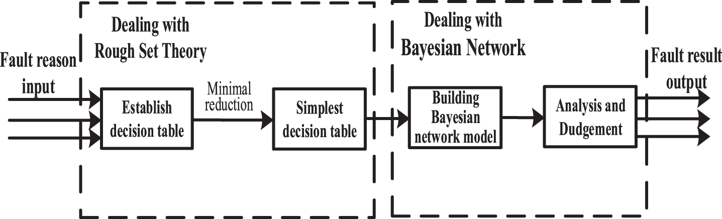
Algorithm block diagram.

Fig. 2

Bayesian network structure block diagram.

The Bayesian probability distribution formula is as follows: $P (X) = \prod_{i = 1}^{n} P (X_{i} | X_{i - 1}, . . ., X_{1})$ (7)

According to the Bayesian network structure in Fig. 2, the child nodes connected to the parent node are independent of each other.

$\begin{matrix} P (X_{1}, X 2, X 3, X 4, X_{5}) \\ = P (X_{1} | X_{5}) \times P (X_{2} | X_{1}, X_{5}) \times P (X_{3} | X_{2}) \\ \times P (X_{4} | X_{5}, X_{2}, X_{3}) \times P (X_{5}) \end{matrix}$ (8)

Aiming at the problem of high-speed loom fault diagnosis, the Bayesian network is constructed according to the following steps [30, 31]:

All the causes and results of high-speed loom faults are expressed as nodes of the network.

It uses directional wires to connect the cause and result of the failure.

The probability of each node can be calculated according to the influence of fault causes on fault results.

Suppose the set U = [X₁, X₂, . . . , Xn, C] is discrete, where X₁, X₂ … , X_n denotes the cause variable, C denotes the result variable, C can take c₁, c₂, . . . , c_n. The failure cause variable X_i can take many values. If the sample Y_i = [x₁, x₂, . . . , x_n], the corresponding failure result c_i probability is: $P (c_{i} | x_{1}, x_{2}, . . ., x_{n}) = \frac{P (x_{1}, x_{2}, . . ., x_{n} | c_{i}) P (c_{i})}{P (x_{1}, x_{2}, . . ., x_{n})}$ (9)

Among them, P (x₁, x₂, . . . , x_n|c_i) P (c_i)/P (x₁, x₂, . . . , x_n) is a Bayesian formula, P (x₁, x₂, . . . , x_n|c_i) is a priori probability, P (c_i) is the total probability of failure result c_i, P (x₁, x₂, . . . , x_n) is the joint probability of failure cause x₁, x₂, . . . , x_n. When calculating the posterior probability of a system, the joint probability β is a fixed value because the fault causes of the system are known as x₁, x₂, . . . , x_n. Then the upper formula can be simplified to: $\begin{matrix} P (c_{i} | x_{1}, x_{2}, \dots, x_{n}) = \frac{P (x_{1}, x_{2}, \dots, x_{n} | c_{i}) P (c_{i})}{P (x_{1}, x_{2}, \dots, x_{n})} \\ = β P (x_{1}, x_{2}, . . ., x_{n} | c_{i}) P (c_{i}) \end{matrix}$ (10)

Because the specific Bayesian network structure can not be determined with only sample data, it is necessary to learn the Bayesian structure.

2.2.1 Structural learning

Assuming that all the learning samples are m, that is, the number of nodes is m, and can form a Bayesian network, then the number of networks is: $f (m) = \sum_{i = 1}^{m} (- 1)^{i + 1} \frac{m!}{(m - 1)! i!} 2^{m + 1 - i} f (m - i)$ (11)

Therefore, it is challenging to retrieve the required network from such a large number of networks, so it is essential to choose an efficient search method. At present, there are two commonly used search methods: scoring optimization and constrained search. The scoring optimization method improves the Bayesian network structure by scoring function, and finally finds the most suitable network model. Although the constraint method is more intuitive, it has higher complexity and is more sensitive to errors. This fault diagnosis system adopts the K2 scoring optimization method:

In the [0,1] interval, there exists a joint probability distribution of several random variables, assuming that there are d variables μ_i, and $\sum_{i = 1}^{d} μ_{i} = 1$ , remember μ = (μ₁, μ₂, . . . , μ_d), each variable μ_i has its corresponding parameter α_i, and α_i > 0, note α = (α₁, α₂, . . . , α_d), $\overset{\land}{α} = \sum_{i = 1}^{d} α_{i}$ .

Then its probability density function is:

$\begin{matrix} p (μ | α) & = Dir (μ | α) \\ = \frac{Γ (\overset{\land}{α})}{Γ (α_{1}) Γ (α_{2}) \cdot \cdot \cdot Γ (α_{d})} \prod_{i = 1}^{d} μ_{i}^{α_{i} - 1} \end{matrix}$ (12)

Its statistics are: $E [μ_{i}] = \frac{α_{i}}{\overset{\land}{α}}$ (13)

$var (μ_{i}) = \frac{α_{i} (\overset{\land}{α} - α_{i})}{{\overset{\land}{α}}^{2} (\overset{\land}{α} + 1)}$ (14)

$cov (μ_{i}, μ_{j}) = \frac{α_{i} α_{j}}{{\overset{\land}{α}}^{2} (\overset{\land}{α} + 1)}$ (15)

Then the probability distribution is Dirichlet distribution. Assuming that the prior probability of parameter β of Bayesian network obeys Dirichlet distribution, then: $P (D | G) = \prod_{i = 1}^{n} \prod_{j = 1}^{q_{i}} \frac{Γ (α_{ij})}{Γ (α_{ij} + N_{ij})} \prod_{k = 1}^{r_{i}} \frac{Γ (α_{ijk} + N_{ijk})}{Γ (α_{ijk})}$ (16) $\begin{matrix} log P (D | G) = \sum_{i = 1}^{n} \sum_{j = 1}^{q_{i}} log (\frac{Γ (α_{ij})}{Γ (α_{ij} + N_{ij})}) \\ + \sum_{k = 1}^{r_{i}} log (\frac{Γ (α_{ijk} + N_{ijk})}{Γ (α_{ijk})}) \\ α_{ij} = \sum_{k} α_{ijk}, N_{ij} = \sum_{k = 1}^{r_{i}} N_{ijk} \end{matrix}$ (17)

2.2.2 Parameter learning

If the network structure is known, the process of parameter learning is scoring by querying historical data or expert knowledge, then deducing the conditional probability of each node in the network, and determining the probability distribution table of nodes.

In the case of incomplete data, it is more difficult to get the appropriate network structure than in the case of complete data. This fault diagnosis system learns from the network when the fault data is incomplete.

2.2.3 Bayesian classifier

Bayesian classifiers are NB (Naive Bayesian Classifier), TAN Bayesian Classifier, GBN (General Bayesian Classifier). The fault diagnosis system uses NB (Naive Bayesian Classifier) model.

NB (Naive Bayesian Classifier) is a classification method based on Bayesian Theorem. It is called “Naive” because it assumes that “the features of the items to be classified are independent of each other,” thus simplifying the problem and effectively reducing the complexity of classification [32, 33]. When the NB (Naive Bayesian Classifier) model is used to calculate the probability of high-speed loom failure, the total probability p (C_j) of each fault in the sample is calculated first, and the frequency of the fault occurrence can calculate the prior probability of the fault, that is: $p (C_{j}) = \frac{N_{C_{j}}}{N}$ (18) $p (Y = x_{i} | C_{j}) = \frac{N_{C_{j}}^{(x_{i})}}{N_{C_{j}}}$ (19)

Among them, $N_{C_{j}}^{(x_{i})}$ is the frequency of the fault result C_j and the fault reason x_i, and N_{C
_j} is the frequency of the fault result C_j. When $N_{C_{j}}^{(x_{i})} = 0$ , the following formula calculates the conditional probability of high-speed loom failure: $p (Y = x_{i} | C_{j}) = \frac{1 / N}{N_{C_{j}} + N_{x_{j}} / N}$ (20)

Through the above method, the probability p (x₁, x₂, . . . , x_n|c_j) p (c_j) of all the fault results in sample Y_i = [x₁, x₂, . . . , x_n] is calculated, and the final diagnosis result is found to be the most probable fault result.

3 Building fault diagnosis model of high-speed loom

3.1 Causes and results of common faults

A high-speed loom system is a complex system that integrates machinery and electricity. Given the different faults of high-speed looms, there is occasionality between faults and fault causes. A fault may be caused by one or more fault causes, and a fault cause may also cause one or more faults [34, 35]. High-speed loom faults include mechanical and electrical faults. Because the probability of mechanical faults is minimal and the signal acquisition is difficult, this paper mainly analyses and diagnoses the electrical faults of high-speed looms. The high-speed loom is a system. When something goes wrong, the situation becomes very complicated.

By consulting the literature and debugging on-site, this paper sorted out the common causes of high-speed loom faults, solutions and results of faults. They are shown in Tables 1 and 2.

Table 1
Type of cause of failure

No. Failure cause type No. Failure cause type

C ₁ Weft Storage Fault C ₆ Coiling Servo Failure

C ₂ Weft Detector Fault C ₇ Electronic Dobby Fault

C ₃ The fault of Weft Selection Device C ₈ The fault of Tension Sensor

C ₄ The fault of Winding Mechanism C ₉ Troubleshooting Sensor Fault

C ₅ Let-off Servo Failure C ₁₀ Inverter Fault

No.	Failure cause type	No.	Failure cause type
C ₁	Weft Storage Fault	C ₆	Coiling Servo Failure
C ₂	Weft Detector Fault	C ₇	Electronic Dobby Fault
C ₃	The fault of Weft Selection Device	C ₈	The fault of Tension Sensor
C ₄	The fault of Winding Mechanism	C ₉	Troubleshooting Sensor Fault
C ₅	Let-off Servo Failure	C ₁₀	Inverter Fault

Table 2

Fault result types

Fault No.	Fault result type	Fault No.	Fault result type
A ₁	Broken Weft	A ₆	Underparking
A ₂	Broken Channel	A ₇	Inadequate Suction of Slow Clutch
A ₃	Excessive Tension	A ₈	Inadequate Suction of Main Clutch
A ₄	Too Little Tension	A ₉	Inadequate Suction of Weft Clutch
A ₅	Double Weft	A ₁₀	Weft-finding is not in Place

Tables 1 and 2 number the common failure causes and failure result in types of high-speed loom respectively, to facilitate the subsequent processing by rough set and Bayesian theory. The cause and result of the failure are not merely corresponding. For example, the fault of let off the servo and take-up servo can cause the fault of let off, and at the same time, it may lead to the phenomenon that the tension is too large or too small. In order to get an accurate fault result type, we need to apply the follow-up algorithm for analysis and processing.

In the actual work, the acquisition of fault causes is uploaded to the remote server after the local operation is completed. We can judge whether the running state of each part of the loom is healthy by the circuit hardware detection system developed by ourselves, and obtain the data source of fault judgment.

3.2 Fault diagnosis model based on rough set and bayesian theory

In the process of high-speed loom fault diagnosis, rough set theory is applied to reduce attributes of fault causes and results to find the minimum reduction and classification rules, and then the Bayesian fault diagnosis network model is built according to classification rules. Finally, the probability of each fault reason is calculated by the Bayesian fault diagnosis network, and the maximum probability of the fault reason is the final diagnosis. Figure 3 is the flow chart of fault diagnosis.

Fig. 3

Fault diagnosis flowchart.

In this paper, the prior probability p (C_i) of high-speed loom fault results and the strength of fault cause set are obtained by analyzing nearly 500 high-speed loom fault data that were collected in the field. Because there are few electrical data of high-speed loom at present, some subjective experience is temporarily added to the causal relationship between the cause and result of some faults [36 –38]. The prior probability table of high-speed loom faults is shown in Table 3.

Table 3

Lever failure prior probability table

Failure Cause No.	Prior Probability	Failure Cause No.	Prior Probability
C ₁	0.265	C ₆	0.118
C ₂	0.004	C ₇	0.005
C ₃	0.032	C ₈	0.013
C ₄	0.025	C ₉	0.281
C ₅	0.132	C ₁₀	0.012

The prior probability in Table 3 refers to the probability of fault occurrence obtained from previous experience and analysis. It is an inference based on the existing knowledge. It comes from subjective experience estimation. A proper and accurate prior probability of fault can improve the accuracy of fault diagnosis of the high-speed loom.

The strength table of the causality of high-speed loom faults is shown in Table 4.

Table 4

High-speed loom failure causality strength table

No.	A ₁	A ₂	A ₃	A ₄	A ₅	A ₆	A ₇	A ₈	A ₉	A ₁₀
C ₁	0.69	0	0	0	0.23	0	0	0.07	0	0
C ₂	0.38	0	0	0	0.66	0	0	0	0	0
C ₃	0.89	0	0	0	0	0	0	0	0	0
C ₄	0	0.63	0	0.93	0	0	0	0.91	0.09	0
C ₅	0	0.76	0	0.94	0	0	0	0	0	0.05
C ₆	0	0.88	0.18	0.18	0	0	0	0	0	0.11
C ₇	0	0.03	0.49	0.49	0	0	0	0	0	0
C ₈	0	0	0.35	0.33	0	0	0.23	0.19	0.08	0
C ₉	0	0.71	0	0.11	0	0	0.23	0.19	0.08	0
C ₁₀	0.12	0	0	0	0	0.9	0.86	0.77	0	0.01

Table 4 shows the connection between the failure cause and failure result, that is, the probability P (A_j|C_j) of A_j in the case of failure C_j. The above table is equivalent to the decision table when using rough sets. The data in the table is a constant value. First, the data must be processed into discrete data. The size of the data reflects the strength of the causal relationship between X and A. Here, R_ijis used to represent the strength of the relationship between them.

To discretize the values in the table:

0 < R_ij ⩽ 0.25, R_ij = 1;

0.25 < R_ij ⩽ 0.5, R_ij = 2;

0.5 < R_ij ⩽ 0.75, R_ij = 3;

0.75 < R_ij ⩽ 1, R_ij = 4;

The decision table of high-speed loom fault diagnosis is shown in Table 5.

Table 5

High-speed loom Failure Decision Table

No.	A ₁	A ₂	A ₃	A ₄	A ₅	A ₆	A ₇	A ₈	A ₉	A ₁₀
C ₁	3	0	0	0	1	0	0	1	0	0
C ₂	2	0	0	0	2	0	0	0	0	0
C ₃	4	0	0	0	4	0	0	0	0	0
C ₄	0	2	0	1	0	0	0	1	1	0
C ₅	0	4	0	4	0	0	0	0	0	1
C ₆	0	4	4	1	0	0	0	0	0	1
C ₇	0	1	1	1	0	0	0	0	0	0
C ₈	0	0	2	2	0	0	0	0	0	0
C ₉	0	3	0	1	0	0	0	1	1	0
C ₁₀	1	0	0	0	0	1	4	4	0	1

Applying rough set theory to attribute reduction of Table 5, two minimum attribute sets {A₁, A₂, A₃, A₅, A₆, A₈, A₉} and {A₁, A₂, A₄, A₅, A₆, A₈, A₉} are obtained. Select {A₁, A₂, A₃, A₅, A₆, A₈, A₉} as the minimum reduction. The minimum reduction is shown in Table 6.

Table 6

Minimum reduction

No.	A₁.	A ₂	A ₃	A ₅	A ₆	A ₈	A ₉
C ₁	3	0	0	0	0	1	0
C ₂	2	0	0	2	0	0	0
C ₃	4	0	0	4	0	0	0
C ₄	0	2	0	0	0	1	1
C ₅	0	4	0	0	0	0	0
C ₆	0	4	4	0	0	0	0
C ₇	0	1	1	0	0	0	0
C ₈	0	0	2	0	0	0	0
C ₉	0	3	0	0	0	1	1
C ₁₀	1	0	0	0	1	4	0

According to the relationship between fault causes and fault results in Table 6, a network model based on NB (Naive Bayes) is constructed, as shown in Fig. 4.

Fig. 4

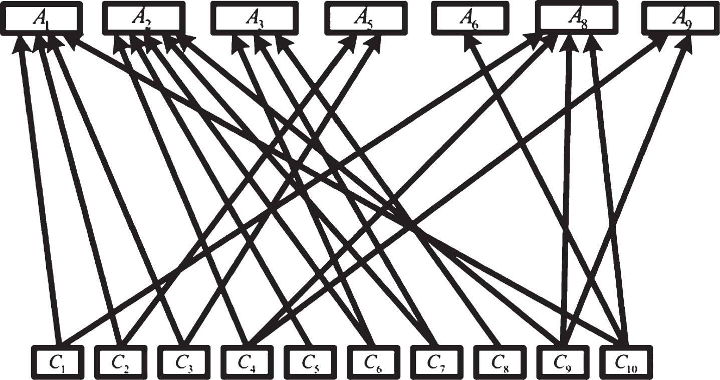
Lobe fault Bayesian model.

From Fig. 4, it can be seen that there is uncertainty between the causes and results of high-speed loom faults, which is a one-to-one, many-to-many relationship. Then the model is learned, because the sensor information of the high-speed loom is not detected at the same time, but detected at different angles when the spindle of the high-speed loom moves to different angles, so this paper uses incremental learning method to make the node information better expressed in the network. Figure 5 is a Bayesian network learning structure.

Fig. 5

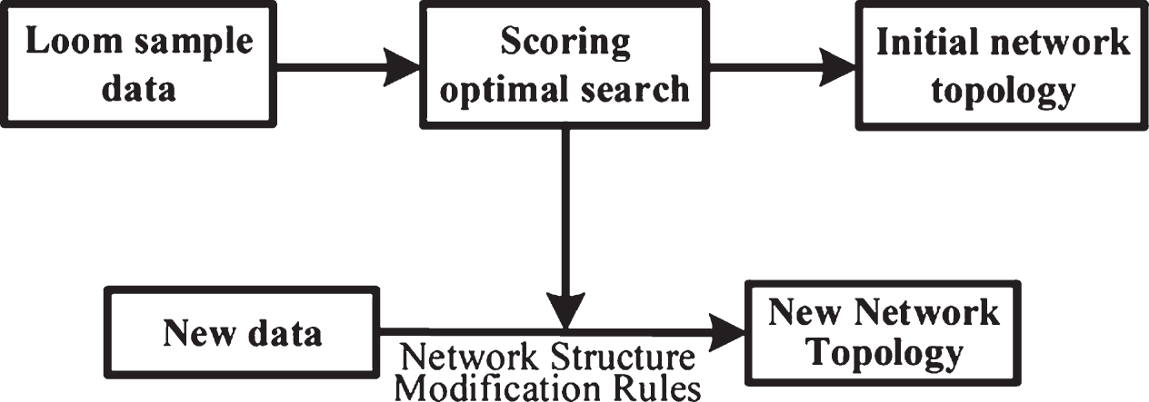
Bayesian network structure learning.

4 Simple examples and effects comparison

4.1 A simple example of fault diagnosis

Following is an example to verify the feasibility of the high-speed loom fault diagnosis model:

In a certain experiment, when the high-speed loom stops due to weft breakage in normal operation, it stops at the weft stopping angle, that is, A₁ = 1, A₂ = 0, A₃ = 0, A₅ = 0, A₇ = 0, A₈ = 0, A₉ = 0. Combining the High-speed loom Fault Causality Intensity Table and Fault Prior Probability Table, the probability of each fault condition is obtained as follows: $\begin{matrix} P (C_{1} | A_{1}, A_{2}, A_{3}, A_{5}, A_{6}, A_{8}, A_{9}) \\ = α P (C_{1}) \prod_{(i = 1)}^{n} P (A_{i} | C_{1}) \\ = α P (C_{1}) P (A_{1} | C_{1}) [1 - P (A_{2} | C_{1})] [1 - P (A_{3} | C_{1})] \\ [1 - P (A_{5} | C_{1})] [1 - P (A_{6} | C_{1})] \\ [1 - P (A_{8} | C_{1})] [1 - P (A_{9} | C_{1})] \\ = α \times 0 . 265 \times 0 . 69 \times (1 - 0) \times (1 - 0) \times (1 - 0 . 23) \\ \times (1 - 0 . 07) \times (1 - 0) = 0 . 13094 α \end{matrix}$

Similarly available: $\begin{matrix} P (C_{2} | A_{1}, A_{2}, A_{3}, A_{5}, A_{6}, A_{8}, A_{9}) \\ = α P (C_{2}) \prod_{i = 1}^{n} P (A_{i} | C_{2}) = 0.00052 α \\ P (C_{3} | A_{1}, A_{2}, A_{3}, A_{5}, A_{6}, A_{8}, A_{9}) \\ = α P (C_{3}) \prod_{i = 1}^{n} P (A_{i} | C_{3}) = 0.02848 α \\ P (C_{4} | A_{1}, A_{2}, A_{3}, A_{5}, A_{6}, A_{8}, A_{9}) \\ = α P (C_{4}) \prod_{i = 1}^{n} P (A_{i} | C_{4}) = 0 \\ P (C_{5} | A_{1}, A_{2}, A_{3}, A_{5}, A_{6}, A_{8}, A_{9}) \\ = α P (C_{5}) \prod_{i = 1}^{n} P (A_{i} | C_{5}) = 0 \\ P (C_{6} | A_{1}, A_{2}, A_{3}, A_{5}, A_{6}, A_{8}, A_{9}) \\ = α P (C_{6}) \prod_{i = 1}^{n} P (A_{i} | C_{6}) = 0 \\ P (C_{7} | A_{1}, A_{2}, A_{3}, A_{5}, A_{6}, A_{8}, A_{9}) \\ = α P (C_{7}) \prod_{i = 1}^{n} P (A_{i} | C_{7}) = 0 \\ P (C_{8} | A_{1}, A_{2}, A_{3}, A_{5}, A_{6}, A_{8}, A_{9}) \\ = α P (C_{8}) \prod_{i = 1}^{n} P (A_{i} | C_{8}) = 0 \\ P (C_{9} | A_{1}, A_{2}, A_{3}, A_{5}, A_{6}, A_{8}, A_{9}) \\ = α P (C_{9}) \prod_{i = 1}^{n} P (A_{i} | C_{9}) = 0 \\ P (C_{10} | A_{1}, A_{2}, A_{3}, A_{5}, A_{6}, A_{8}, A_{9}) \\ = α P (C_{10}) \prod_{i = 1}^{n} P (A_{i} | C_{10}) = 0.00003 α \end{matrix}$

From $\sum_{i = 1}^{10} P (C_{i} | A_{1}, A_{2}, A_{3}, A_{5}, A_{6}, A_{8}, A_{9}) = 1$ , α = 6.2512 is obtained.

Therefore: $P (C_{1} | A_{1}, A_{2}, A_{3}, A_{5}, A_{6}, A_{8}, A_{9}) = 0.8185$ $P (C_{2} | A_{1}, A_{2}, A_{3}, A_{5}, A_{6}, A_{8}, A_{9}) = 0.0033$ $P (C_{3} | A_{1}, A_{2}, A_{3}, A_{5}, A_{6}, A_{8}, A_{9}) = 0.1780$ $P (C_{4} | A_{1}, A_{2}, A_{3}, A_{5}, A_{6}, A_{8}, A_{9}) = 0$ $P (C_{5} | A_{1}, A_{2}, A_{3}, A_{5}, A_{6}, A_{8}, A_{9}) = 0$ $P (C_{6} | A_{1}, A_{2}, A_{3}, A_{5}, A_{6}, A_{8}, A_{9}) = 0$ $P (C_{7} | A_{1}, A_{2}, A_{3}, A_{5}, A_{6}, A_{8}, A_{9}) = 0$ $P (C_{8} | A_{1}, A_{2}, A_{3}, A_{5}, A_{6}, A_{8}, A_{9}) = 0$ $P (C_{9} | A_{1}, A_{2}, A_{3}, A_{5}, A_{6}, A_{8}, A_{9}) = 0$ $P (C_{10} | A_{1}, A_{2}, A_{3}, A_{5}, A_{6}, A_{8}, A_{9}) = 0.0002$

After the above calculation, the probability of P (C₁|A₁, A₂, A₃, A₅, A₆, A₈, A₉) is the highest, so the diagnosis result is the fault of weft accumulator. In the field fault detection, weft storage is found to be short of yarn, which results in weft breakage stopping and is consistent with the diagnosis results.

Using this method to diagnose high-speed loom fault has the advantage of high fault-tolerant rate. Even if the phenomenon of misdiagnosis occurs, it can also be sorted according to the probability calculated in the process of diagnosis, and then it can be repaired, which greatly reduces the workload of maintenance personnel.

4.2 Comparison of Several Fault Diagnosis Methods

The feasibility of fault diagnosis method for high-speed looms based on rough set and Bayesian is verified above, but the accuracy is not proved yet. In this paper, “Weka” (software for data mining) is used to simulate common fault diagnosis methods and fault diagnosis systems using rough set and Bayesian combination of fault diagnosis methods, and then verify the accuracy of fault diagnosis, through statistical diagnosis of the correct number of samples to calculate the accuracy of diagnosis.

Among the table, the “*” represents the missing high-speed loom attributes.

Table 7 is reduced by rough set theory, and Table 8 is the minimum reduction.

Table 7
High-speed loom Failure Data Sheet

No. A ₁ A ₂ A ₃ A ₄ A ₅ A ₆ A ₇ A ₈ A ₉ A ₁₀ Number

C ₁ 3 0 0 0 * 0 0 1 0 0 163

C ₂ 2 0 0 0 3 0 0 0 0 0 12

C ₃ 4 1 1 0 * 0 0 1 0 0 19

C ₄ 0 2 1 0 0 0 1 0 0 0 13

C ₅ 0 4 0 4 0 0 0 0 0 * 66

C ₆ 0 4 4 * 0 0 1 0 0 1 59

C ₇ 0 * 1 * 0 0 0 0 1 0 4

C ₈ 0 0 2 2 0 0 0 0 0 0 8

C ₉ 0 3 0 1 0 0 1 0 * 0 150

C ₁₀ * 0 0 0 1 0 4 4 0 1 6

No.	A ₁	A ₂	A ₃	A ₄	A ₅	A ₇	A ₈	A ₉	A ₁₀	Number
C ₁	3	0	0	0	*	0	1	0	0	163
C ₂	2	0	0	0	3	0	0	0	0	12
C ₃	4	1	1	0	*	0	1	0	0	19
C ₄	0	2	1	0	0	1	0	0	0	13
C ₅	0	4	0	4	0	0	0	0	*	66
C ₆	0	4	4	*	0	1	0	0	1	59
C ₇	0	*	1	*	0	0	0	1	0	4
C ₈	0	0	2	2	0	0	0	0	0	8
C ₉	0	3	0	1	0	1	0	*	0	150
C ₁₀	*	0	0	0	1	4	4	0	1	6

Table 8

High-speed loom Failure Data Table After Attribute Reduction

No.	A ₁	A ₂	A ₃	A ₅	A ₆	A ₈	A ₉	Number
C ₁	3	0	0	*	0	1	0	163
C ₂	2	0	0	3	0	0	0	12
C ₃	4	1	1	*	0	1	0	19
C ₄	0	2	1	0	0	0	0	13
C ₅	0	4	0	0	0	0	0	66
C ₆	0	4	4	0	0	0	0	59
C ₇	0	*	1	0	0	0	1	4
C ₈	0	0	2	0	0	0	0	8
C ₉	0	3	0	0	0	0	*	150
C ₁₀	*	0	0	1	0	4	0	6

In the table, the “*” represents the missing high-speed loom attributes.

“Weka” software is used to train and simulate the samples of Naive Bayesian Network, Neural Network and Decision Tree. The number of training samples and test samples are shown in Table 9. Moreover, the simulation results are shown in Fig. 6.

Table 9

The Distribution of Sample Number

Failure Cause Type	No.	Number of Training Sample	Number of Test Samples
Weft Storage Fault	C ₁	99	64
Weft Detector Fault	C ₂	7	5
The fault of Weft Selection Device	C ₃	11	8
The fault of Winding Mechanism	C ₄	8	5
Let-off Servo Failure	C ₅	40	26
Coiling Servo Failure	C ₆	35	24
Electronic Dobby Fault	C ₇	2	2
The fault of Tension Sensor	C ₈	5	3
Troubleshooting Sensor Fault	C ₉	90	60
Inverter Fault	C ₁₀	3	3

Fig. 6

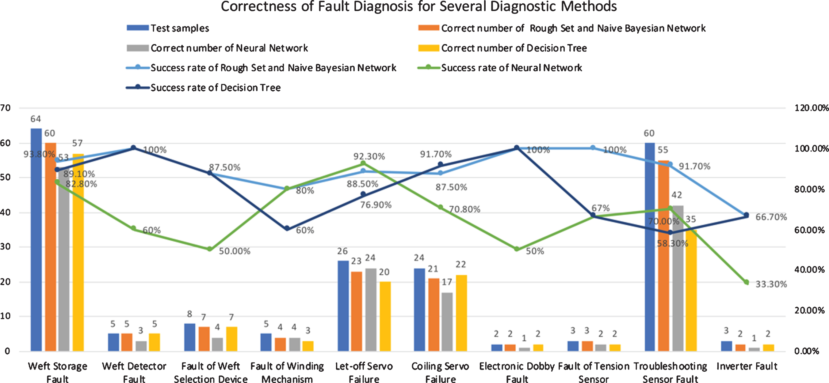
The correctness of Fault Diagnosis for Several Diagnostic Methods.

Figure 6 shows that in the case of incomplete fault data of high-speed loom, the fault diagnosis accuracy of naive Bayesian network simplified by rough set theory is much higher than that of decision tree and neural network, with an average accuracy of 89.6%. Moreover, the accuracy of the fault diagnosis method fluctuates less, which means that the algorithm has high stability.

The false alarm is an important parameter to improve detection accuracy. The false alarm rate of several diagnosis methods is calculated by large-scale data simulation. The results are shown in Fig. 7.

Fig. 7

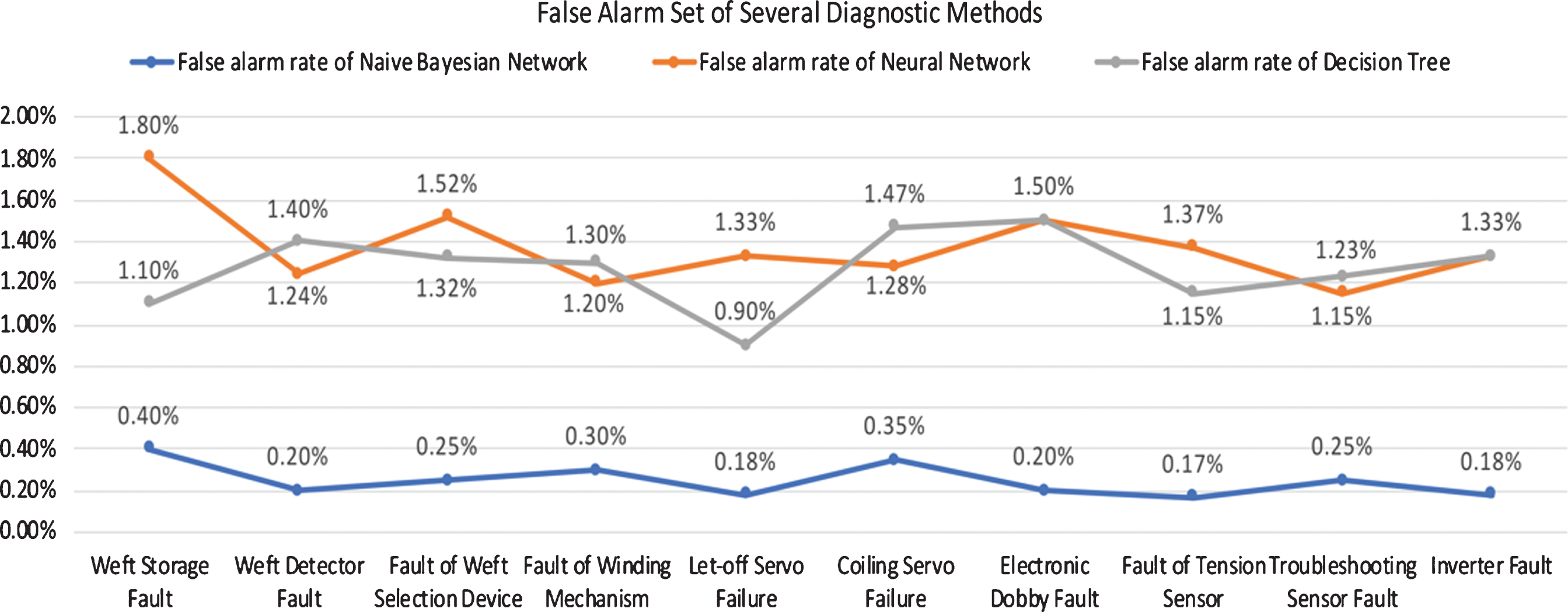
False Alarm of Several Diagnostic Methods.

As can be seen from Fig. 7, the fault diagnosis method of rough set and Bayesian network is used to get a low false alarm rate, which proves the high detection accuracy of this method from another perspective.

In conclusion, in the fault diagnosis system of the high-speed loom, the method of combining rough set and Bayesian networks not only has higher diagnosis accuracy, but also has a lower false alarm rate, which proves that the performance of this method is superior.

4.3 Robustness of the Algorithm

For a system, if facing any fault, the system does not exceed the permitted scope of the index and can meet the needs of users, then the system is robust.

In order to test the robustness of the algorithm, this paper adopts software fault injection technology. Because the high-speed loom belongs to a mature and stable industrial machine, and there will be no high concurrent faults, so we give up the pressure test and mainly use the method of error information input to test the robustness of the algorithm. 800 error information generated randomly and 200 fault reasons collected on-site for fault diagnosis tests are taken as input and transmitted to the fault diagnosis system to compare the accuracy of the diagnosis results. In order to judge the robustness of the algorithm. The initial success rate and the current success rate are shown in Fig. 8.

Fig. 8

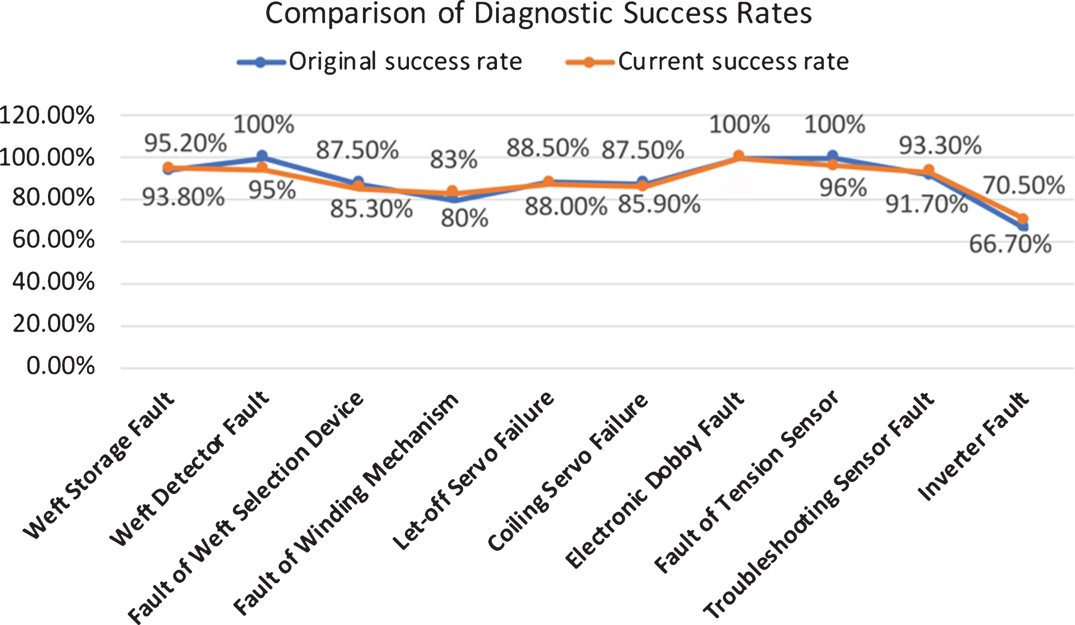
Comparison of Diagnostic Success Rates.

It can be seen from Fig. 8 that even if a large amount of wrong information is input, the diagnosis success rate of the fault diagnosis system only fluctuates within a limited range, and the deviation of the diagnosis result obtained is not significant, which proves that the algorithm has good robustness.

5 Conclusions

Through a comprehensive analysis of a high-speed loom system, this paper mainly introduces the results, causes and solutions of common high-speed loom faults. In this paper, rough set theory and its attribute reduction method, Bayesian network theory, and its network model building method are briefly introduced. A high-speed loom fault diagnosis model based on rough set theory and Bayesian network is constructed. Then the feasibility of the model is proved by an example. The reason for the failure is determined by the production field control system through the circuit hardware detection method to determine the operation status of each part of the high-speed loom. After the failure reason is found, it is transferred to the remote cloud server. Further fault detection is carried out on the remote server. When the fault detection system on the remote server receives the fault information, it will not directly process it, but first trigger a status flag bit and timer, when it receives the same fault information again after a while, it will process the information. This can ensure that the input is reliable fault information, not a false alarm. In the whole process of system processing, the hardware detection and network status of the production site are maintained. All of these ensure that the algorithm is stable and reliable. A large number of missing or incomplete high-speed loom fault data are collected in the field. The naive Bayesian network, neural network and decision tree are trained, studied and verified by data mining software Weka. Firstly, rough set theory is used to reduce the fault data of high-speed loom. Then train the data. After the training and learning of the naive Bayesian network, the fault reason data is input to get the fault result. The accuracy of the method is 89.6%, and the false alarm rate is about 0.2%. In this paper, the method of wrong input is used to analyze the robustness of the system algorithm. Even if there is a large number of wrong input interference, the diagnosis system can still work typically, and the success rate of diagnosis fluctuates in a limited range, which proves that the system algorithm has good robustness Compared with other methods, the results of rough set and naive Bayesian network are better than other methods. It shows that the fault diagnosis system has better performance under the condition of incomplete data and missing information.

Footnotes

ACKNOWLEDGMENTS

This work was supported by the National Key Instrument and Equipment Development of the National Key R&D Program of China (Grant No. 2017YFF0106404), the National Natural Science Foundation of China (Grant No. 51675160), the Hebei key research and development plan project (Grant No. 18214407D), and the Tianjin Science and Technology Commissioner Project (Grant No. H0302).

References

Meng

, Wu

and Gray

, Machine-to-Machine Connectivity, Messaging, and Understanding for Future Digital Manufacturing Industry, Sensors, 17 2694 (2017), 1–15.

Henao

, et al., Trends in Fault Diagnosis for Electrical Machines: A Review of Diagnostic Techniques, In IEEE Industrial Electronics Magazine 8(2) (2014), 31–42.

and Chen

, The designer of control system for rapier high-speed loom based on CAN bus, Manufacturing Automation 33 (2011), 135–137.

Xiao

, Wang

, Yang

and Gao

, Multiple faults diagnosis in motion system based on SVM, International Journal of Machine Learning and Cybernetics 3(1) (2012), 77–82.

Watanabe

, Hirota

, Hou

and Himmeblau

D.M.

, Diagnosis of multiple simultaneous fault via hierarchical artificial neural networks, American Institute of Chemical Engineers Journal 40(5) (1994), 839–848.

and Zhang

, Fault Diagnosis Knowledge Base Optimization Based on Decision Tree. 2018 10th International Conference on Intelligent Human-Machine Systems and Cybernetics (IHMSC), Hangzhou, (2018), pp. 324–327.

Wang

, Wu

, Zhang

and Shi

, Hydraulic system fault diagnosis method based on a multi-feature fusion support vector machine, The Journal of Engineering 13 (2019), 215–218.

Hang

, Zhang

and Cheng

, Application of multi-class fuzzy support vector machine classifier for fault diagnosis of wind turbine, Fuzzy Sets and Systems 297 (2016), 128–140.

Simani

and Turhan

, Fault Diagnosis of a Wind Turbine Simulated Model via Neural Networks**Invited paper for the special session on “Industrial Fault Diagnosis and Fault-tolerant Control” organised by Christophe Aubrun and Vicenc Puig, IFAC-PapersOnLine 51 (2018), pp. 381–388.

10.

Huang

, Zeng

and Zhang

, Fuel Cell Engine Fault Diagnosis Expert System based on Decision Tree. 2019 IEEE 3rd Information Technology, Networking, Electronic and Automation Control Conference (ITNEC), Chengdu, China, (2019), pp. 282–286.

11.

Khan

and Saha

, Neural network based cycloconverter fault detection using wavelet decomposition. 2017 Third International Conference on Advances in Electrical, Electronics, Information, Communication and Bio-Informatics (AEEICB), Chennai, (2017), pp. 352–356.

12.

, Zhao

, Chen

and Hou

, Oil-immersed Power Transformer Internal Fault Diagnosis Research Based on Probabilistic Neural Network, Procedia Computer Science 83 (2016), 1327–1331.

13.

and Zhang

, Fault Diagnosis Knowledge Base Optimization Based on Decision Tree. 2018 10th International Conference on Intelligent Human-Machine Systems and Cybernetics (IHMSC), Hangzhou, (2018), pp. 324–327.

14.

Qayum , Abdul

Muhammad

and Naseer

Muddasser

, A fast approach for finding design repeat in textile rotary printing for fault detection, The Journal of The Textile Institute 108.1 (2017), 62–65.

15.

Mine

, Seçkin

A.Ç.

and Coşkun

, Production fault simulation and forecasting from time series data with machine learning in glove textile industry, Journal of Engineered Fibers and Fabrics 14 (2019).

16.

Mutlu

and Altuntas

, Hazard and risk analysis for ring spinning yarn production process by integrated fta-fmea approach, Textile and Apparel 29(3) (2019), 208–218.

17.

Mutlu

N.G.

and Altuntas

, Risk analysis for occupational safety and health in the textile industry: Integration of FMEA, FTA, and BIFPET methods, International Journal of Industrial Ergonomics 72 (2019), 222–240.

18.

Gültekin

, Dülger

H.Ç.

, Sünbül

and Kani

, Image Processing Applications on Yarn Characteristics and Fault Inspection,ü, hendis 26(116) (2019), 340–345.

19.

Weldeslasie

D.T.

, Mesfin

, Gronli

T.M.

, Younas

and Ghinea

, An Expert System Approach for the Diagnosis and Rectification of Yarn Faults. In: Awan I., Younas M., Ünal P., Aleksy M. (eds) Mobile Web and Intelligent Information Systems. MobiWIS 2019. Lecture Notes in Computer Science, vol 11673 (2019), Springer, Cham, pp. 230–242.

20.

Chang

, Chen

and Lee

, Inference and diagnosis model based on Bayesian network and rough sets theory. 2014 International Conference on Machine Learning and Cybernetics, Lanzhou, (2014), pp. 455–461.

21.

Xie

, Zeng

, Ruan

, Chen

and Zhang

, Transformer fault diagnosis based on bayesian network and rough set reduction theory. IEEE 2013 Tencon – Spring, Sydney, NSW, (2013), pp. 262–266.

22.

Andhalkar

and Momin

B.F.

, Rough Set Theory and its Extended Algorithms. 2018 Second International Conference on Intelligent Computing and Control Systems (ICICCS), Madurai, India, (2018), pp. 1434–1438.

23.

Kudo

and Murai

, An Attempt of Object Reduction in Rough Set Theory. 2018 Joint 10th International Conference on Soft Computing and Intelligent Systems (SCIS) and 19th International Symposium on Advanced Intelligent Systems (ISIS), Toyama, Japan, (2018), pp. 33–36.

24.

Zheng

, Hu

, Zhan

, Ma

and Qi

, An enhancement for heuristic attribute reduction algorithm in rough set, Expert Systems with Applications 41 (2014), 6748–6754.

25.

Zhang

, Jin

, Zheng

and Jiang

, Mechanical Product Ecological Design Knowledge Reduction Based on Rough Set, Procedia CIRP 80 (2019), 33–38.

26.

Marouane

E.M.

and Houssaine

, Fast outlier detection method based on Rough set. 2018 9th International Symposium on Signal, Image, Video and Communications (ISIVC), Rabat, Morocco, (2018), pp. 60–66.

27.

Song

, Tsang

, Chen

and Yang

, Minimal decision cost reduct in fuzzy decision-theoretic rough set model, Knowledge-Based Systems 126 (2017), 104–112.

28.

Wang

, Shen

and Mei

, Cost sensitive multi-class fuzzy decision-theoretic rough set based fault diagnosis. 2017 36th Chinese Control Conference (CCC), Dalian,(2017), pp. 6957–6961.

29.

Khakzad

, System safety assessment under epistemic uncertainty: Using imprecise probabilities in Bayesian network, Safety Science 116 (2019), 149–160.

30.

Wang

, Yang

, Yuan

and Cao

, An improved Bayesian network method for fault diagnosis, IFAC-Papers OnLine 51 (2018), 341–346.

31.

D’Angelo

, Palhares

, Cosme

, Aguiar

, Fonseca

and Caminhas

, Fault detection in dynamic systems by a Fuzzy/Bayesian network formulation, Applied Soft Computing 21 (2014), 647–653.

32.

Zhao

, Yang

, Diao

, An

, Zhao

and Zhang

, A novel approach to transformer fault diagnosis using IDM and naive credal classifier, International Journal of Electrical Power & Energy Systems 105 (2019), 846–855.

33.

Muralidharan

and Sugumaran

, A comparative study of Naïve Bayes classifier and Bayes net classifier for fault diagnosis of monoblock centrifugal pump using wavelet analysis, Applied Soft Computing 12 (2012), 2023–2029.

34.

Dong

and Shi

, The High-speed loom Monitoring System Design with High Reliability and Easy Maintainability. 2011 International Conference on Control, Automation and Systems Engineering (CASE), Singapore, (2011), pp. 1–5.

35.

Gao

, Cecati

and Ding

, A Survey of fault diagnosis and fault-tolerant techniques—Part II: Fault diagnosis with knowledge-based and hybrid/active approaches, IEEE Trans Ind Electron 62 (2015), 3768–3774.

36.

Meng

, Wu

and Gray

, RFID-based Object-Centric Data Management Framework for Smart Manufacturing Applications, IEEE Internet of Things Journal 6 (2019), 2706–2716.

37.

Cai

, Huang

and Xie

, Bayesian networks in fault diagnosis, IEEE Trans Ind Inform 13(5) (2017), 2227–2240.

38.

, Wang

, Kwong

and Wang

, Bayesian classifiers based on probability density estimation and their applications to simultaneous fault diagnosis, Inf Sci 259 (2014), 252–268.